Electrohydraulic Crimping of Tubes within Rings

Abstract

Crimping processes are commonly used in industry to join two tubular parts together. In the case of positive clearance crimping, one of the two parts must be plastically deformed to fill the initial clearance and block elastic deformations in the second one. The strength of the assembly will then depends on the residual contact pressure established at the interface. Quasi-static processes are the most commonly used to perform these operations, but over the past two decades, there has been a growing interest in the use of dynamic crimping by magnetic pulse. Processes that generate high-strain rate allow to reduce the springback, which is of great interest for crimping. However, its use is limited if the part to be deformed is made of a poor electrical conductor material or if its dimensions are too small. This paper presents an alternative for dynamically crimping tubes within rings using electrohydraulic process. An experimental equipment has been designed to guide and amplify pressure waves to the area to be deformed. Two amplifiers called acoustic and mechanical pulse shapers (APS and MPS) have been tested and allow to reach hoop strain rate at about 1000 and 100 s${}^{-1}$ respectively. An analytical model was also built allowing to define the stored energy and the inter-electrodes distance to maximize the pressure. Results of push-out tests are also presented and demonstrate the ability of the electrohydraulic crimping process coupled with the MPS to crimp small 316L tubes into rings made of the same material, but achieving crimping successfully with the APS still require further work.

1. Introduction

The assembly of tubes between them or with other parts is an important issue in mechanical construction because it is a recurring need in almost all industries. In the field of automotive, railway or military construction, tubular structures are commonly used because they allow the production of light and resistant frames in a simple way [1]. In this case, it is necessary to joint tubes together. In the field of energy, joints between tubes are also encountered, but this time it involves more massive parts. This is generally the case with heat exchangers used in the oil and gas industry or for the production of electrical energy in conventional or nuclear thermal power plants. These joints are also common in the naval defense industry for the propulsion of surface vessels or submarines. Indeed, steam generators and condensers, commonly called tubular exchangers, are devices made up of tubes crimped in tubesheets used to transfer the thermal energy contained in the fluids (more or less radioactive and at different temperatures) which cross them. Tube-to-tubesheet joints play a very important role in terms of safety since they prevent the mixing of primary and secondary fluids. These joints constitute a primary containment barrier [2].

To make these joints, it is possible to use a crimping process. Mori and al. [3] classify crimping processes into two families depending on whether the initial clearance between the parts to be jointed is positive or negative. In the case of crimping by negative clearance, the outer and inner parts can either be press-fitted, or fitted after heating the outer part and/or cooling the inner part. In the case of crimping by positive clearance, one of the two parts must be plastically deformed in order to fill the initial clearance and block elastic strains in the second. The differential springback between the two parts makes it possible to establish a residual contact pressure at the interface and thus to ensure the mechanical strength of the joint. For this, several processes are available: roller expansion which consists in plastically deforming the tube by the mechanical action of rollers; expansion by elastomer compression; hydraulic expansion or even hybrid crimping which combines several processes.

Among the advantages of crimped joints, we can cite: (i) the small size and the speed of execution compared to screw joints; (ii) unlike joining by welding there is no heat affected zone [4]; (iii) no pre- or post-processing is necessary. Research works on crimped joints with a positive initial clearance generally aim to determine the optimum geometric parameters and materials in order to maximize the strength of the crimped joints. Merah [5] explored the effect of initial radial clearance between the tube and the ring while Oppenheimer [6] and Maxwell [7] recommended to use a much higher yield stress for the material of the ring compared to that of the tube. Others works concern the evaluation of the residual contact pressure by analytical models in order to avoid often costly experimental campaigns [8,9,10,11]. To improve the strenght of crimped joints, researchers have also tried to implement a groove inside the ring, as shown by Marré and Wang’s works [1,12]. However, this requires additional machining operations. More recently there has been an interest in dynamic crimping by magnetic pulse. This technology, which consists in plastically deforming a tube made of a material that is a good electric conductor by means of Lorentz forces, has been used successfully for the joint of camshafts [13], for the manufacture of lightweight tubular structures [14] or more simply for cylindrical parts [15]. Faes et al. [16] showed that the magnetic pulse process is a very relevant one for achieving crimped joints with positive clearance with or without grooves. High-strain rate processes allow to reduce the springback [17] which, in the context of crimping, presents an major advantage. Unfortunately, when it comes to deforming a tube in a bore, if the tube is made of a poor electric material conductor or if its diameter is too small, the magnetic pulse process cannot be used.

In the context of this study, we propose to take advantage of the electrohydraulic technology in order to crimp a tube within a bore, but at high strain rates, hence with comparable properties with respect to those observed in magnetic pulse crimping [18]. The electrohydraulic forming process consists in discharging the electrical energy stored in a series of capacitors between two immersed electrodes in a water tank, and to exploit its effects. This discharge creates an electric arc in the water [19], then a plasma, which generates pressure waves that travel in the water. A few microseconds after the discharge, a so-called primary shock wave first appears, followed by a set of so-called secondary pressure waves a few tens of microseconds later, which result from the oscillation of a vapor bubble. To perform forming or crimping operations by electrohydraulic discharge, it is therefore sufficient to ensure that the pressure waves propagate towards the surfaces to be deformed. This process is already used for sheet metal forming operations [20], and it has also been used to perform crimping when the diameter of the tube allows it [21].

To carry out crimping by electrohydraulic discharge of the extremity of a tube of small diameter within a ring, it is necessary to conduct the pressure waves inside the tube while maintaining the magnitude and the rate of the loading. In this article we present an original experimental way to crimp, from the inside, a tube in a ring by electrohydraulic discharge. Two configurations are considered to guide and amplify the pressure waves. Each of these two configurations is successively analyzed and tested experimentally.

2. Equipments

2.1. Material

In this study, we used tubes and rings made of 316L stainless steel in the annealed state. The tubes have an outer diameter $d_o$ = 28 mm, a thickness t = 1.5 mm and a length $L_t$ = 60 mm. The rings have an outer diameter $D_o$ = 43 mm, an inner diameter $D_i$ = 28.1 mm and a width $L_r$ = 25 mm.

Table 1. Chemical composition of stainless steel 316L.

%C	%Mn	%P	%S	%Si	%Cr	%Ni	%Mo	%N	%O	%Fe
<0.03	<2	<0.01	<0.005	<1	<16–19	<10.5–13	<1.5–3	<0.003	<0.002	Compl

presents the chemical composition of this alloy.

2.2. Pulsed Current Generator

To power our crimping system, a pulsed current generator developed at Ecole Centrale Nantes is used which can store a maximum energy of 46 kJ. It has the following features: $C_{Gen}$ = 408 $\mathsf{\mu }$F; $L_{Gen}$ = 0.1 $\mathsf{\mu }$H; $R_{Gen}$ = 3 m$\mathsf{\Omega }$; $U_{max}$ = 15 kV; $I_{max}$ = 500 kA, where $C_{Gen}$, $L_{Gen}$, $R_{Gen}$, $U_{max}$ and $I_{max}$ denote the capacitance, inductance, resistance, maximum load voltage and maximum short-circuit current respectively. Energy switching is performed with ignitrons.

2.3. Crimping System

Figure 1 presents a schematic diagram of the experimental electrohydraulic crimping equipment which has been the subject of a patent [22]. It consists of three sub-systems: (i) a waves generator that generates high intensity pressure waves in water; (ii) a pulse shaper which shapes the time evolution of the pressure wave, and guides it to the desired location; (iii) a crimping probe [23]. The waves generator consists of two insulated electrodes (1) and an electrohydraulic discharging tank (2). The pressure amplifier or pulse shaper (3) is used to guide and/or amplify the pressure waves emitted by the waves generator. A crimping probe opened on the periphery by means of gills (4) allows to conduct the pressure waves inside a tube to crimp within a ring. High-pressure valves controlled by compressed air using pneumatic valves permit to control the inlets/outlets of water and air in the system while isolating the control system from any returns of eddy currents. A liquid ring vacuum pump, which can draw in air and water, evacuates the gases retained in the crimping probe during the placement of the tube and ring.

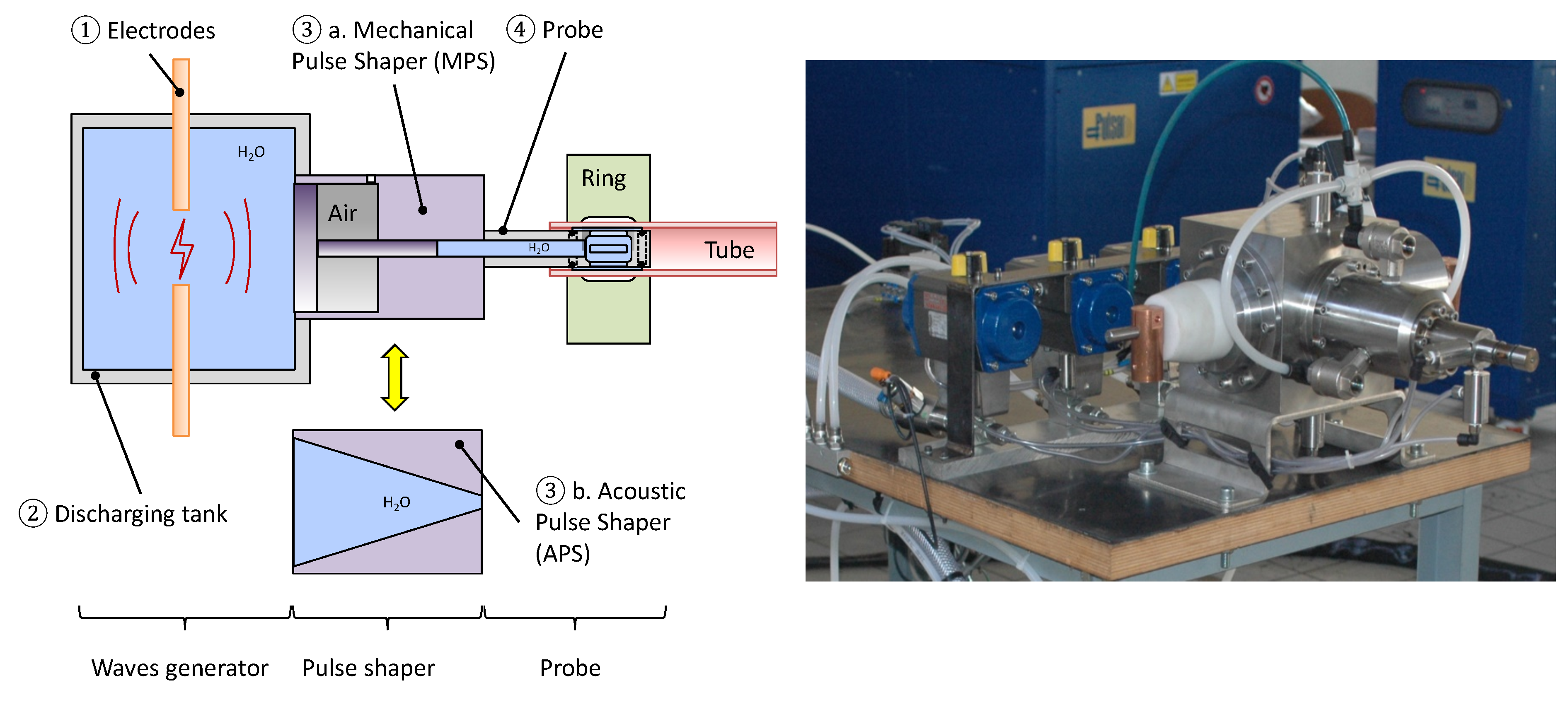
2.4. Waves Generator

The waves generator consists of a discharging tank and two electrodes. Bonnen et al. [19] have shown that electrodes erosion is a significant phenomenon of degradation of the wave generator in electrohydraulic processes. Even if the pointed geometry is the most efficient since it permits to intensify the electric field by point effect [24], 100C6 steel electrodes whose end is cylindrical (diameter 8 mm) were preferred in this study. This is mainly because, unlike the case of a tip, the wear of a cylindrical shape does not significantly modify the geometry of the end of the electrode. Since their erosion is inevitable, the adjustment of the inter-electrodes distance must be carried out regularly. The charging circuit of the pulsed current generator, which can be modeled by a voltage generator, a capacitance $C_{Gen}$ (capacitor bank) and a switch, makes it possible to charge the capacities to a voltage value $U_0$, in order to store the electrical energy $E_0$ defined as:

$$E_0=\frac{1}{2}{C}_{Gen}{U_0}^2.$$

(1)

Once the capacities are charged, the charging circuit is opened and the discharge circuit is closed. By employing an ignitron-type high-voltage switch, the energy stored in the capacitors can be rapidly transferred between the two electrodes in a few microseconds. The discharge circuit can be modeled, from an electrical point of view, by an RLC circuit which leads to the following time evolution of the current [24]:

$$i\left(t\right)=I_0{\mathrm{e}}^{-t/\tau }sin\left({\omega }_{0}t\right),$$

(2)

with $I_0\simeq U_0\sqrt{C_{Gen}/L_0}$, $\tau =2L_0/R_0$, ${\omega }_0=1/\sqrt{L_0{C}_{Gen}}$ and where $L_0$, $R_0$ designate the inductance and resistance of the discharge circuit, respectively.

Timoshkin’s results [25] show that the resistance of the plasma $R_{arc}$ is between 20 m$\mathsf{\Omega }$ and 200 m$\mathsf{\Omega }$ for switched currents of the same order of magnitude than those reached during the present study. Thus, the resistance of the circuit $R_0$ is defined such as:

$$R_0=R_{Gen}+R_{arc}.$$

(3)

Kushner [26] was also interested in measuring the inductance of the plasma $L_{arc}$ and he was thus able to show that it was negligible compared to that of the circuit $L_0$ (generator + cables), which was experimentally evaluated at 1.22 $\mathsf{\mu }$H.

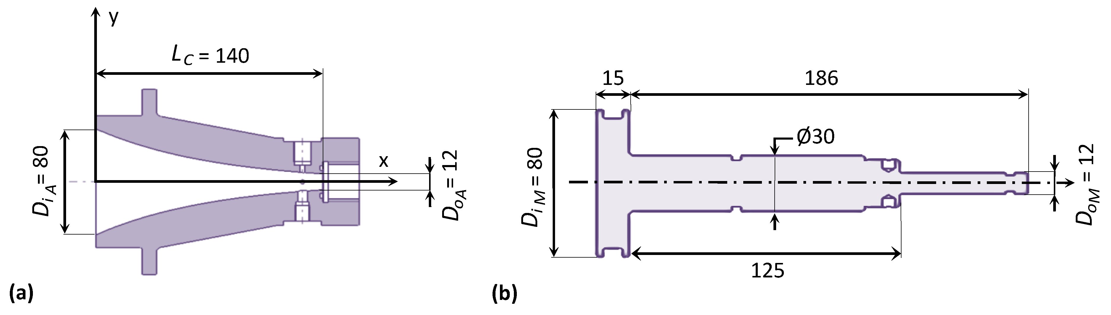
2.5. Acoustic and Mechanical Pulse Shapers

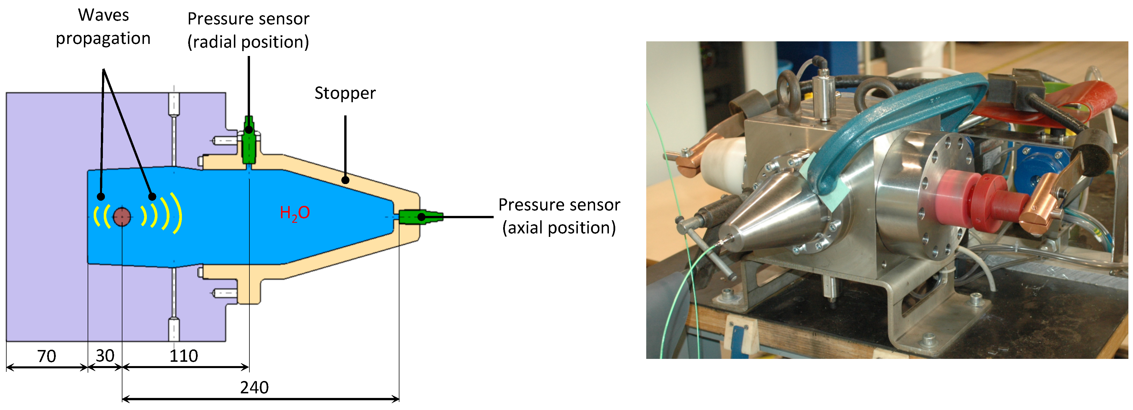
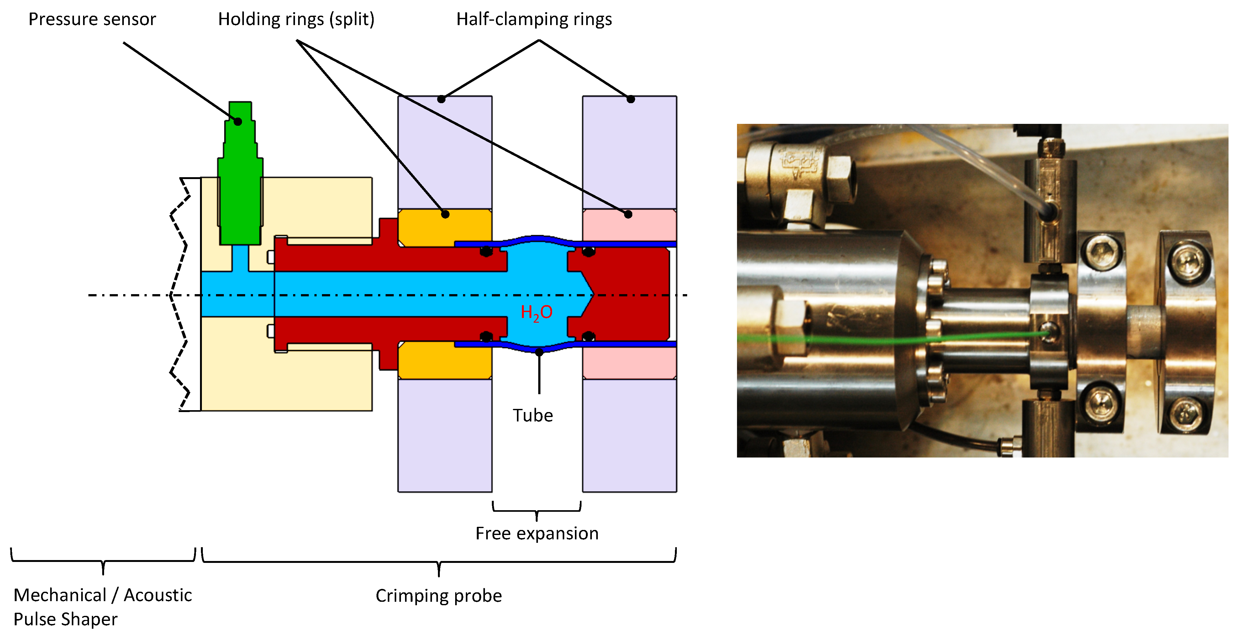
Two different pulse shapers are proposed here, whose geometries are shown in Figure 2, and can be combined with the aforementioned wave generator. The first one is the acoustic pulse shaper (APS), shown in Figure 2a. Its purpose is to conduct and focus the energy of the shock wave towards the input of the crimping probe. According to Mercier or Wang [27,28], an exponential evolution of the cross-section or of its diameter with the longitudinal coordinate is the most suitable one. Given the input ${D_i}_A$ and output ${D_o}_A$ diameters of the acoustic amplifier, it must follow the following profile:

$$D\left(x\right)={D_i}_A{\mathrm{e}}^{-\alpha x}\mathrm{with}\alpha =-\frac{1}{L_c}ln\left(\frac{{D_i}_A}{{D_o}_A}\right).$$

(4)

Figure 2b presents the second pulse shaper, which is the mechanical pulse shaper (MPS). It consists of a piston, on which the pressure waves emitted from the wave generator first act on its larger diameter, then propagate along the rod before being transmitted to the crimping probe. Although rather known for quasi-static processes, this two-sided piston will here play the role of a filter and of an amplifier of waves emitted by the waves generator, since many wave round trips will occur along the rod as the piston moves forward due to the input pressure pulse. Its static amplification ratio is here set to about 44. Before each test using the MPS and once the tube is placed on the probe, the following operations are performed: the piston is moved back, the air is evacuated from the probe and the waves generator vessel, the probe and the tank are finally filled with water.

2.6. Crimping Probe

The crimping probe conducts the pressure waves coming out of the pulse shaper to the inside of the crimped tube (Figure 3). Four gills, as well as a reduction in the diameter of the probe between two O-rings, allow the pressure to be applied inside the tube.

2.7. Means of Measurement

To measure the discharge current, a Rogowski CWT1500 PEM (Power Electronic Measurements, Nottingham, UK) probe is used. This probe can measure maximum current peaks of 300 kA and maximum peaks of current rate $di/dt$ peaks of 40 kA $\mathsf{\mu }$s${}^{-1}$.

The voltage measurement at the electrode terminals was performed using Tektronix P6015A voltage probes. These probes can measure DC voltages up to 20 kV and transient voltages up to 40 kV. They have a bandwidth of 75 MHz.

The pressure was measured using a quartz sensor marketed by Kistler (model 6213B). This sensor has a measurement range from 0 to 10,000 bar, and a bandwidth of 150 kHz. During the tests, the passage of an intense current between the electrodes generates significant eddy currents in the tank. In order to avoid any current feedback via the measurement chain, the pressure sensor amplifier and oscilloscope are battery powered and not grounded.

To determine the strain rate of the tube during the free expansion test, a fast camera Photron Fastcam SA 1.1 is used to perform a surface tracking. Its acquisition speed varies between 5400 frames per second for a resolution of 1024 × 1024 pixels and 675,000 frames per second for a resolution of 64 × 16 pixels. For our observations, we chose a resolution of 256 × 128 pixels, which allowed us to have an acquisition speed of 125,000 frames per second, or one image every 8 microseconds.

3. Methods

3.1. Experimental Set-Up for Measuring the Input/Output Law of the Waves Generator

To measure the input/output law of the waves generator (evolution of the pressure as a function of the discharge energy and the inter-electrodes distance), a stopper is used on which it is possible to position the pressure sensor either axially at the end of the stopper or radially at its inlet (Figure 4).

3.2. Experimental Set-Up for Expansion Pressure Measurement

Figure 5 shows the experimental set-up used to measure the pressure applied to the outlet of the crimping probe at the gills. A thick ring, supposedly rigid, is fitted on the probe and the sensor is positioned on it.

3.3. Experimental Set-Up for Strain Rate Measurements during a Free Expansion Test

Figure 6 shows the free expansion device used to measure the strain rate in the tube. It consists of two thick holding rings that block the radial displacement of the tube. The tube is free to expand between these two rings at the crimping probe’s gills. A high-speed camera allows to measure the temporal evolution of the radius of the tube $U_r\left(t\right)$. Since the tube is thin, the hoop strain can be assumed to be uniform in the thickness of the tube, so it is possible to deduce the maximum hoop strain rate from the displacement measurements.

3.4. Experimental Set-Up for Crimping Tests

Figure 7 shows the experimental set-up used for crimping tests. The tube (1) is fitted to the crimping probe (2). Two O-rings (3) ensure the seal between the tube and the crimping probe. Two retaining rings (4) and two clamping rings (5) block the radial displacement of the tube at the seals. The crimped ring (6) is fitted on the tube between the two holding rings, which positions it axially opposite to the gills of the crimping probe.

4. Results and Discussion

4.1. Input/Output Waves Generator Law

Figure 8 presents the evolution of the peak discharge current $I_{max}$ as a function of the inter-electrodes distance e for each level of discharge energy $E_0$. Several observations can be made:

• the more the allowable inter-electrodes distance, the more the discharge energy;
• the more the inter-electrodes distance, the more the dispersion;
• for a given energy, the maximum intensity of the current decreases as the inter-electrodes distance increases.

Table 2. Limit conditions for the initiation of an electric arc.

${\mathit{E}}_0$ (kJ)	${\mathit{e}}_{\mathit{l}}$ (mm)	$\parallel {\overrightarrow{\mathit{E}}}_{\mathit{l}}\parallel$ (kV/m)
2	2	1.57 × 10${}^3$
6	3	1.81 × 10${}^3$
8	4	1.57 × 10${}^3$
10	4	1.75 × 10${}^3$

gathers the inter-electrodes limit distances $e_l$ beyond which it is no longer possible to initiate the discharge. Since the inter-electrodes distance has been increased by increments of 0.5 mm, the actual limit distance ${e_l}_{real}$ lies between the values listed in Table 2, and their incremented values with a pitch of 0.5 mm, i.e.,:

$$e_l\le {e_l}_{real}\le e_l+0.5 \mathrm{mm}.$$

(5)

The electric field occurring between the electrodes can be approximated by the following expression:

$$\overrightarrow{E}=-\overrightarrow{grad}\left(U\right)\simeq {\displaystyle \frac{U_0}{e_l}}{\overrightarrow{e}}_z,$$

(6)

where ${\overrightarrow{e}}_z$ denotes the direction joining the two electrodes. The inter-electrodes limit distance for each energy level $E_0$ being known, the charging voltage can be deduced from the energy (Equation (1)) with the following expression:

$$U_0=\sqrt{\frac{2E_0}{C_{Gen}}}.$$

(7)

The limit magnitude of the electric field $\parallel {\overrightarrow{E}}_l\parallel$ beyond which the discharge is no longer possible can be calculated for each of the energy levels. The limit electric field thus varies between 1570 kV m${}^{-1}$ and 1810 kV m${}^{-1}$ (Table 2). Given the uncertainty in the measurement of the limit inter-electrodes distance mentioned above, the electric field corresponding to the limit inter-electrodes distance for different energy levels is reasonably constant (about 1670 kV m${}^{-1}$). The experimental results obtained are therefore qualitatively consistent. This limit electric field value corresponds to the case of a subsonic discharge [29], i.e., for an electric field less than 60,000 kV m${}^{-1}$. Indeed, in this study the maximum field reached is 7000 kV m${}^{-1}$ for an energy of 10 kJ and for an inter-electrodes distance of 1 mm, which corresponds well to a subsonic regime. These results allow to validate the plasma formation mechanism, namely that a gaseous channel is formed between the two electrodes under the effect of the electric discharge and that the ionization of this channel leads to the creation of the plasma.

Figure 9 presents the typical pattern of current and voltage signals between the electrodes of the waves generator during a test. If we note $U_0$ the charging voltage of the capacitances, we can see that the voltage value $U_1$ corresponding to the moment when the current will flow in the plasma is significantly lower than $U_0$. The energy consumed to form the plasma therefore corresponds to:

$$\Delta E=E_0-E_1={\displaystyle \frac{1}{2}}{C}_{Gen}({U_0}^2-{U_1}^2),$$

(8)

where $E_1$ is the available energy after the formation of the plasma. Moreover, as demonstrated above, the formation of the plasma is all the more difficult as the inter-electrodes distance is high. Therefore, the more the inter-electrodes distance, the more the consumed energy $\Delta E$. From Equation (2), the maximum current $I_{max}$ can be expressed as a function of the inductance of the circuit and the energy stored in the capacitances as:

$$I_{max}=i\left(\frac{T}{4}\right)=U_1\sqrt{\frac{C_{Gen}}{L_0}}{\mathrm{e}}^{-\pi \frac{R_0}{4}\sqrt{\frac{C_{Gen}}{L_0}}}.$$

(9)

It is therefore logical that the maximum current decreases as the inter-electrode distance increases, since it varies linearly with $U_1$, which itself decreases with that distance. On the other hand, since the formation of the plasma is more difficult when approaching the inter-electrodes limit distance, it is also not surprising that the uncertainties about the current intensity or the pressure are greater. Indeed, a slight error in adjusting the inter-electrodes distance can significantly modify the fraction of energy required for the formation of the plasma and therefore the amount of energy actually deposited in the plasma.

Figure 10 presents the evolution of the shock pressure $P_{sh}$ measured with the sensor in axial position using the set-up presented Figure 4 as a function of the inter-electrodes distance e and the charging energy $E_0$. It is observed that the pressure increases with both the discharge energy and the inter-electrodes distance. To interpret this evolution, it is necessary to establish the relationship linking the pressure to the energy and the inter-electrodes distance.

The discharge of capacities occurs as soon as the plasma is formed, which by Joule effect, allows the deposition of the electrical energy in the form of heat. The energy $E_{arc}$ required to create an electrical arc thus reads:

$$E_{arc}={\int }_0^{t_f}{R}_{arc}{i}^{2}dt,$$

(10)

where $R_{arc}$ denotes the electrical resistance of the plasma (=electric arc) and $t_f$ the duration of the discharge.

The time evolution of the current being known (Equation (2)), we will assume, as a first approximation, that the deposition and therefore the discharge is made during the first half-period of the current $t_f$:

$$t_f=\frac{T}{2}=\pi \sqrt{L_0{C}_{Gen}}.$$

(11)

If we assume that, during the discharge, a cylindrical plasma channel of diameter d and of length equal to the inter-electrodes distance e is formed, then the resistance of the plasma is written:

$$R_{arc}=\frac{{\rho }_{arc}e}{\pi d^2/4},$$

(12)

where ${\rho }_{arc}$ refers to the resistivity of plasma. Although this is a very strong and quite unrealistic assumption, the objective of this analysis is not to calculate the value of the pressure but rather its dependence on the operating parameters, which has no consequences on the result. Under these conditions the energy deposited in the plasma is written as:

$$E_{arc}\simeq \frac{{\rho }_{arc}e}{\pi d^2/4}{\int }_0^{T/2}{i}^{2}dt.$$

(13)

The development of Equation (13), detailed in the Appendix A, leads to a new expression of $E_{arc}$ such as:

$$E_{arc}\simeq \frac{{\rho }_{arc}e}{\pi d^2/4}\frac{E_1}{R_0}\left(1-{\mathrm{e}}^{-\pi R_0\sqrt{\frac{C_{Gen}}{L_0}}}\right).$$

(14)

At a distance r much greater than the inter-electrodes distance e, the wavefront can be modelled as a spherical surface S of radius r. The power developed by the pressure wave is then given by the expression:

$$P_w={\int }_S{P}_{sh}{u}_{p}dS,$$

(15)

where $P_{sh}$ is the pressure of the shock wave and $u_p$ the material velocity in the considered medium (the water in this case) during the propagation of the shock wave. These two quantities being uniform on the front of the wave, we can then write:

$$P_w=4\pi r^2{P}_{sh}{u}_p.$$

(16)

The shock pressure is given by the following expression (Rankine-Hugoniot equation of the conservation of linear momentum) [28]:

$$P_{sh}={\rho }_0{u}_s{u}_p,$$

(17)

where ${\rho }_0$ is the density of water, and $u_s$ the speed of the shock. In addition, the shock speed in water is a function of the properties of the medium, and is usually approximated by the following equation of state:

$$u_s=c_0+S{u}_p,$$

(18)

where $c_0$ and S denote the sound speed in water and some coefficient identified experimentally respectively. By assuming that $u_s$ is constant (i.e., for moderate pressure levels), the power can be expressed as:

$$P_w=4\pi r^2\frac{{P_{sh}}^2}{{\rho }_0{u}_s}.$$

(19)

Since the energy deposition is supposed to occur over half a period of the current, the power can be written as the ratio between the energy deposited in the plasma and half of the discharge period:

$$P_w=\frac{E_{arc}}{T/2}.$$

(20)

In practice, not all of the energy deposited in the plasma is transmitted to the shock wave. Laforest [30] estimates, for example, that 15% of heat conduction losses occur in the electrodes, and that 30% of losses take place in the plasma in the form of radiation. If we note $\alpha$ the fraction of the energy transmitted to the shock wave, then equating the Equations (19) and (20) and accounting for Equation (14), it allows to deduce the expression of the shock pressure $P_{sh}$ as a function of the process parameters:

$$P_{sh}\sim A\sqrt{e\alpha E_1}\frac{1}{r},$$

(21)

with:

$$A=\frac{1}{\pi \sqrt{\pi }}\sqrt{{\rho }_0{u}_s}\frac{\sqrt{{\rho }_{arc}}}{d}\frac{1}{\sqrt{R_0\sqrt{L_0{C}_{Gen}}}}\sqrt{\left(1-{\mathrm{e}}^{-\pi R_o\sqrt{\frac{C_{Gen}}{L_0}}}\right)}.$$

(22)

The pressure of the primary shock wave therefore diverges geometrically (evolution in 1/r), which is due to the effect of spherical dispersion [31], and is proportional to the square root of the energy and to the square root of the inter-electrodes distance. The results shown in Figure 10 thus allow to define the energy/inter-electrodes distance parameters (to maximize the pressure while maintaining reasonable uncertainties) that will be used in the rest of the study.

Figure 11 presents the time recordings of the signals of the pressure and of the current during a test conducted at 8 kJ with an inter-electrodes distance of 2.5 mm when the crimping probe is closed by means of a rigid ring using the set-up presented in Figure 5 with the APS (Acoustic Pulse Shaper). This signal is characteristic of an electrohydraulic discharge: a shock wave is first emitted, followed by secondary waves resulting from the oscillations of the vapor bubble. The first pressure wave (the shock wave) arrives on the sensor 208 $\mathsf{\mu }$s after the beginning of the discharge, which approximately corresponds to the propagation time of the acoustic waves in water at the speed of 1480 m s${}^{-1}$ between the center of the electrodes and the position of the sensor (287 mm). The maximum pressure level of 320 MPa is reached after 300 $\mathsf{\mu }$s after the beginning of the discharge, which is the pressure resulting from the summation of the various incident and reflected waves in the waves generator. The secondary waves, with amplitudes of less than 30 MPa, arrive on the sensor 2 ms after the beginning of the discharge.

Figure 12 presents the pressure signal measured at the outlet of the crimping probe closed by a rigid ring and the current signal during a test conducted at 8 kJ with an inter-electrode distance of 2.5 mm using the set-up presented Figure 5 with the MPS (Mechanical Pulse Shaper). We do not observe any shock wave anymore but only what seems to be an image of the secondary waves emitted by the waves generator that have been amplified. The first pressure wave arrives at the sensor about 340 $\mathsf{\mu }$s after the beginning of the discharge and reaches a level of 103 MPa. The pressure waves cross now various media, each having their own sound speed (1480 m s${}^{-1}$ in water and 5900 m s${}^{-1}$ in steel), which theoretically should make the first wave arrive 138 $\mathsf{\mu }$s after the discharge. However, this calculation does not take into account the time elapsed between the emission of the shock wave and the formation of the vapor bubble responsible for the secondary waves. It should also be noted that from one test to another, the amplitude and the number of oscillations may vary.

During electrohydraulic discharge, a shock wave is emitted from the center of the electrodes and propagates towards the piston with the MPS. Figure 13a presents the different media crossed by the shock wave. Coming from the water tank, it first crosses the piston made of steel, and is then transmitted to the water of the crimping probe. However, the presence of the piston will shape the pulse transmitted to the latter through various wave transmissions and reflections. In order to get a first sketch of the process of wave reflections occurring within the piston, the simplified one-dimensional modeling shown in Figure 13b may be considered at first. It consists of a stack of media $A/B/A$, supposed infinite in transverse directions, where the medium A corresponds to water and the medium B corresponds to steel.

Consider an incident wave disturbance of intensity $\Delta {\sigma }_i$ travelling from a medium A towards a medium B. When this wave disturbance reaches the interface between the media A and B, part of the wave is reflected (with an intensity $\Delta {\sigma }_r$) and another part is transmitted (of intensity $\Delta {\sigma }_t$). Using the method of characteristics, the intensity of the transmitted and reflected wave disturbances between the two media A and B can be expressed as a function of the intensity of the incident wave disturbance as [28]:

$$\Delta {\sigma }_t=2\frac{{\rho }_B{C}_B}{{\rho }_A{C}_A+{\rho }_B{C}_B}\Delta {\sigma }_i=T_{AB}\Delta {\sigma }_i,$$

(23)

$$\Delta {\sigma }_r=\frac{{\rho }_B{C}_B-{\rho }_A{C}_A}{{\rho }_A{C}_A+{\rho }_B{C}_B}\Delta {\sigma }_i=R_{AB}\Delta {\sigma }_i.$$

(24)

where $T_{AB}$ and $R_{AB}$ denote the transmission and reflection coefficients, associated with a propagation from A to B [31]. It should be noted that the attenuation of waves due to their dispersions in the material is not taken into account in this approach. Considering the material properties of the water (${\rho }_{water}$ = 1000 kg m${}^{-3}$ and $C_{water}$ = 1480 m s${}^{-1}$) and of steel (${\rho }_{steel}$ = 7600 kg m${}^{-3}$ and $C_{steel}$ = 5800 m s${}^{-1}$), Equations (23) and (24) show that when the wave disturbance passes from water to steel, most of it is transmitted to steel, while when it passes from steel to water, only a very small part of it is transmitted. This is so because the wave material impedance $Z_i={\rho }_i{C}_i$, $i=A,B$ of the water is much lower than that of steel, so that their ratio tends to zero. In other words, the transmission and reflection coefficients T and R appearing in Equations (23) and (24) will tend to 2 and 1 respectively for a propagation from water to steel, and to zero and −1 respectively for a propagation from steel to water.

Given an initial shock wave with associated material velocity $v_0$ and pressure $P_0=Z_{water}{v}_0$, Figure 14 shows the diagram (velocity, pressure) of the mechanical states reached in the piston during wave reflections. It can be seen that after few wave reflections within the medium B (steel), the states transmitted to the water of the crimping probe converge to an equilibrium state $P_A=Z_{water}{v}_A$ and $v_A=v_0$ identical to the input state. The latter initially transported by a shock wave has thus been transmitted to the water of the crimping probe, but in a smoother way because states denoted $2,4,6$ in Figure 14 up to state $(v_A,P_A)$ are successively transmitted. The piston having a length of 201 mm, the part of the shock wave that is transmitted in the water of the crimping probe is done over a duration of about 3.5 ms per pulse of 70 $\mathsf{\mu }$s, which corresponds to the small disturbances observed on the pressure rise phase of the signal of the Figure 12. The piston thus regulates the rise in pressure like a low-pass filter.

It should also be noted that the previous modeling is a very simplified one. A more refined one should actually account for the various changes of cross-sections the piston consists of, which generate many wave reflections and transmissions. This system could therefore be considered as a multi-stage transmission unit. In particular, the propagation of a wave disturbance from a large cross-section to a smaller one yields a magnification of the transmitted stress, so that the smaller segment acts as a wave trap [31].

4.2. Strain Rate Measurement

In order to evaluate the strain rate achieved using the electrohydraulic crimping means, free expansion tests were carried out with an energy $E_0=$ 10 kJ and an inter-electrodes distance $e=$ 3 mm, using the set-up shown in Figure 6. Using the fast camera, we measured the temporal evolution of the radial displacement component $U_r$ of the outer surface of the tube. It is therefore possible to deduce the temporal evolution of the maximum hoop strain as follow:

$${ϵ}_{\theta }=ln\left({\displaystyle \frac{d}{d_0}}\right)=ln\left(1+\frac{2U_r}{d_0}\right).$$

(25)

The hoop strain rate can therefore be deduced and evaluated at about 1133 s${}^{-1}$ with the APS and 148 s${}^{-1}$ with the MPS, which corresponds to a dynamic strain regime. Figure 15 and Figure 16 shows the pressure signal obtained during the same test at 10 kJ with the MPS. Several observations can be made:

• only one pressure wave is present;
• the pressure signal is no longer pseudo-periodic, as it was the case when the crimping probe was equipped with a thick ring (Figure 12), but rather trapezoidal;
• this signal includes a phase of rise that seems to be almost linear but disturbed then a pseudo-plateau and finally a phase of linear decay.

4.3. Crimping Tests

In order to evaluate the effectiveness of the device for crimping a tube in a ring in each of the two configurations (APS and MPS), crimping tests were carried out using the device presented in Figure 7. The crimped joints obtained are shown in Figure 17. A charging energy ranging from 6 kJ to 16 kJ and a launch gap (clearance between the outer surface of the tube and the inner surface of the ring) of 0.1 mm, 0.2 mm and 0.3 mm were tested, repeating each test a minimum of three times. Note that with the APS, regardless of the launch gap, it was not possible to crimp the tube for a value of energy less than 16 kJ. Similarly, with the MPS, it was not possible to crimp below 8 kJ.

Figure 18 shows the evolution of the maximum push-out force as a function of the expansion pressure $P_e$ measured during the tests. Several observations can be made.

• With APS, the measured maximum force is less than 1 kN and no trend can be observed regarding the launch gap.
• With the MPS, for pressures lower than those applied with APS, the maximum push-out force reach up to 7 kN. This seems to show that the intensity of the pressure wave is not enough to achieve a crimping, it is necessary that the load is applied for a sufficiently long time. The MPS, which exploits secondary waves rather than the primary shock wave, is therefore logically more efficient.
• With MPS we find that the lower the launch gap is, the better the crimping is.

5. Conclusions

In this study we present an original experimental device which allows crimping at high strain rate, from the inside, a tube in a ring. The system consists of a waves generator by electro-hydraulic discharge, a pressure amplifier called pulse shaper which has the function of amplifying the pressure waves coming from the wave generator and a crimping probe which has the function of guiding the pressure waves from the pulse shaper inside the tube to be crimped.

The detailed analysis of the functioning of each of these sub-elements allowed us: (i) to understand the influence of the operating parameters (discharge energy, arc distance, inter-electrode distance) on the shock pressure; (ii) to understand the operation of the two pulse shapers studied (low pass filter for the mechanical amplifier and high pass filter for the acoustic amplifier); (iii) to evaluate the strain rates in the crimped zone (of the order of 100 s${}^{-1}$ with the mechanical amplifier and of the order of 1000 s${}^{-1}$ with the acoustic amplifier for a discharge energy of 10 kJ and an inter-electrode distance of 3 mm).

The crimping tests demonstrated the ability of the electrohydraulic crimping process to crimp small 316L tubes into rings made of the same material, when coupled with MPS. However, achieving crimping successfully with the APS still require further work. with the APS still require further work.

References

1. Marré, M.; Rautenberg, J.; Tekkaya, A.E.; Zabel, A.; Biermann, D.; Wojciechowski, J.; Przybylski, W. An experimental study on the groove design for joints produced by hydraulic expansion considering axial or torque load. Mater. Manuf. Process. 2012, 27, 545–555. [Google Scholar] [CrossRef]
2. Jawad, M.H.; Clarkin, E.J.; Schuessler, R.E. Evaluation of Tube-to-Tubesheet Junctions. J. Press. Vessel Technol. 1987, 109, 19–26. [Google Scholar] [CrossRef]
3. Mori, K.-I.; Bay, N.; Fratini, L.; Micari, F.; Tekkaya, A.E. Joining by plastic deformation. CIRP Ann.-Manuf. Technol. 2013, 62, 673–694. [Google Scholar] [CrossRef]
4. Varis, J.P. The suitability of round clinching tools for high strength structural steel. Thin-Walled Struct. 2002, 40, 225–238. [Google Scholar] [CrossRef]
5. Merah, N.; Al-Zayer, A.; Shuaib, A.; Arif, A. Finite element evaluation of clearance effect on tube-to-tubesheet joint strength. Int. J. Press. Vessel. Pip. 2003, 80, 879–885. [Google Scholar] [CrossRef]
6. Oppenheimer, P.H. Rolling tubes in boiler plates. J. Am. Soc. Nav. Eng. 1927, 39, 417–426. [Google Scholar]
7. Maxwell, C.A. Practical aspects of making expanded joints. Trans. ASME 1943, 65, 506–522. [Google Scholar] [CrossRef]
8. Kohlpaintner, W.R. Calculation of hydraulically expanded tube-To-Tubesheet joints. J. Press. Vessel Technol. Trans. ASME 1995, 117, 24–30. [Google Scholar] [CrossRef]
9. Podhorsky, M.; Krips, H. Hydraulic Expansion of Tubes. VGB Kraftwerkstechnik 1979, 1, 77–83. [Google Scholar]
10. Goodier, J.N.; Schoessow, G.J. The holding power and hydraulic tightness of expanded tube joints: Analysis of the stress and deformation. Trans. ASME 1943, 65, 489–496. [Google Scholar] [CrossRef]
11. Yokell, S. Expanded, and welded-and-expanded tube-to-tubesheet joints. J. Press. Vessel Technol. Trans. ASME 1992, 114, 157–165. [Google Scholar] [CrossRef] [Green Version]
12. Wang, H.F.; Sang, Z.F. Effect of geometry of grooves on connection strength of hydraulically expanded tube-to-tubesheet joints. J. Press. Vessel Technol. Trans. ASME 2005, 127, 430–435. [Google Scholar] [CrossRef]
13. Park, Y.-B.; Kim, H.-Y.; Oh, S.-I. Design of axial/torque joint made by electromagnetic forming. Thin-Walled Struct. 2005, 43, 826–844. [Google Scholar] [CrossRef]
14. Hammers, T.; Marré, M.; Rautenberg, J.; Barreiro, P.; Schulze, V.; Biermann, D.; Brosius, A.; Tekkaya, A.E. Influence of mandrel’s surface and material on the mechanical properties of joints produced by electromagnetic compression. Steel Res. Int. 2009, 80, 366–375. [Google Scholar]
15. Kumar, R.; Kore, S.D. Experimental Studies on the Effect of Different Field Shaper Geometries on Magnetic Pulse Crimping in Cylindrical Configuration. Int. J. Adv. Manuf. Technol. 2019, 105, 4677–4690. [Google Scholar] [CrossRef]
16. Faes, K.; Zaitov, O.; De Waele, W. Electromagnetic pulse crimping of axial form fit joints. In Proceedings of the 5th International Conference on High Speed Forming, Dortmund, Germany, 24–26 April 2012. [Google Scholar]
17. Psyk, V.; Risch, D.; Kinsey, B.L.; Tekkaya, A.E.; Kleiner, M. Electromagnetic forming—A review. J. Mater. Process. Technol. 2011, 211, 787–829. [Google Scholar] [CrossRef]
18. Sow, C.T. Etude et Développement du Procédé de Sertissage électrohydraulique. Ph.D. Thesis, Ecole Centrale de Nantes, Nantes, France, 2018. [Google Scholar]
19. Bonnen, J.J.F.; Golovashchenko, S.F.; Dawson, S.A.; Mamutov, A.V. Electrode Erosion Observed in Electrohydraulic Discharges Used in Pulsed Sheet Metal Forming. J. Mater. Eng. Perform. 2013, 22, 3946–3958. [Google Scholar] [CrossRef] [Green Version]
20. Mamutov, A.V.; Golovashchenko, S.F.; Bonnen, J.J.F.; Gillard, A.J.; Dawson, S.A.; Maison, L. Electrohydraulic forming of light weight automotive panels. In Proceedings of the 7th International Conference on High Speed Forming, Dortmund, Germany, 27–28 April 2016. [Google Scholar]
21. Priem, D.; Marya, S.; Racineux, G. On the forming of metallic parts through electromagnetic and electrohydraulic processing. Adv. Mater. Res. 2007, 15, 655–660. [Google Scholar]
22. Priem, D.; Racineux, G.; Manoharan, P. Electro-Hydraulic Forming Machine for the Plastic Deformation of a Projectile Part of the Wall of a Workpiece to be Formed. U.S. Patent 10,413,957, 17 September 2019. [Google Scholar]
23. Le Mentec, R.; Sow, C.T.; Heuzé, T.; Racineux, G. Electrohydraulic Crimping of 316L Tube in a 316L Thick Ring. In Proceedings of the 9th International Conference on High Speed Forming, Dortmund, Germany, 13 October 2021. [Google Scholar]
24. Martin, J. Etude et Caractérisation D’onde de Pression Générée par une Décharge Électrique Dans L’eau. Application à la Fracturation Électrique de Roches. Ph.D. Thesis, Université de Pau et des Pays de l’Adour, Pau Cedex, France, 14 June 2013. [Google Scholar]
25. Timoshkin, I.V.; Fouracre, R.A.; Given, M.J.; MacGregor, S.J. Hydrodynamic modelling of transient cavities in fluids generated by high voltage spark discharges. J. Phys. D Appl. Phys. 2006, 39, 4808. [Google Scholar] [CrossRef]
26. Kushner, M.J.; Kimura, W.D.; Byron, S.R. Arc resistance of laser-triggered spark gaps. J. Appl. Phys. 1985, 58, 1744–1751. [Google Scholar] [CrossRef]
27. Wang, F.; Zhao, X.; Zhang, D.; Wu, Y. Development of novel ultrasonic transducers for microelectronics packaging. J. Mater. Process. Technol. 2009, 209, 1291–1301. [Google Scholar] [CrossRef]
28. Meyers, M.A. Dynamic Behavior of Materials; John Wiley & Sons: New York, NY, USA, 1994. [Google Scholar]
29. Touya, G. Contribution à L’étude Expérimentale des déCharges Électriques Dans L’eau et des Ondes de Pression Associées. Réalisation d’un Prototype Industriel 100 kJ pour le Traitement de Déchets par Puissances Électriques Pulsées. Ph.D. Thesis, Université de Pau et des Pays de l’Adour, Pau Cedex, France, 2003. [Google Scholar]
30. Laforest, Z. Etude Expérimentale et Numérique d’un arc Électrique Dans un Liquide. Ph.D. Thesis, Université Paul Sabatier, Toulouse, France, 2017. [Google Scholar]
31. Wang, L. Foundations of Stress Waves, 1st ed.; Elsevier: Edinburgh, UK, 2007. [Google Scholar]
Figure 1. Schematic of electrohydraulic crimping equipment.
Metals 13 01382 g001
Figure 2. (a) Acoustic and (b) Mechanical Pulse Shapers (units are millimeters).
Metals 13 01382 g002
Figure 3. Crimping probe (unit are millimeters).
Metals 13 01382 g003
Figure 4. Experimental set-up for waves generator input/output law measurement (unit are millimeters).
Metals 13 01382 g004
Figure 5. Experimental set-up for measuring the pressure at the outlet of the crimping probe.
Metals 13 01382 g005
Figure 6. Experimental set-up for free expansion tests.
Metals 13 01382 g006
Figure 7. Experimental set-up for crimping tests.
Metals 13 01382 g007
Figure 8. Evolution of the maximum discharge current I m a x as a function of the inter-electrodes distance e and the discharge energy E 0 .
Metals 13 01382 g008
Figure 9. Measure of the discharge current I and the voltage U between the electrodes of the waves generator.
Metals 13 01382 g009
Figure 10. Evolution of the pressure P s h as a function of the inter-electrodes distance e and the discharge energy E 0 .
Metals 13 01382 g010
Figure 11. Time evolution of the expansion pressure P e at the outlet of the crimping probe closed by a rigid ring with the APS (E = 8 kJ; e = 2.5 mm).
Metals 13 01382 g011
Figure 12. Time evolution of the expansion pressure P e at the outlet of the crimping probe closed by a rigid ring with the MPS (E = 8 kJ; e = 2.5 mm).
Metals 13 01382 g012
Figure 13. Propagation of waves through different media.
Metals 13 01382 g013
Figure 14. Diagram (velocity, pressure) of the mechanical states reached in the piston.
Metals 13 01382 g014
Figure 15. Pictures taken by the high-speed camera during free expansion test with the MPS (E = 10 kJ; e = 3 mm).
Metals 13 01382 g015
Figure 16. Time evolution of the expansion pressure P e at the outlet of the crimping probe during free expansion of the tube with the MPS (E = 10 kJ; e = 3 mm).
Metals 13 01382 g016
Figure 17. Illustration of crimped joints.
Metals 13 01382 g017
Figure 18. Evolution of the maximum push-out force as a function of the expansion pressure P e measured during crimping tests.
Metals 13 01382 g018