Abstract
Simulations of industrial roll-forming processes using the finite element method typically require an extremely fine discretization to obtain accurate results. Running those models using a classical finite element method usually leads to suboptimal meshes where some regions are unnecessarily over-refined. An alternative approach consists in creating non-conformal meshes where a number of nodes, called hanging nodes, do not match the nodes of adjacent elements. Such flexibility allows for more freedom in mesh refinement, which results in the creation of more efficient simulations. Consequently, the computational cost of the models is decreased with little to no impact on the accuracy of the results. Handling the generated hanging nodes can, however, be challenging. In this work, details are first given about the implementation of these particular meshes in an implicit finite element code with a special focus on the treatment of hanging nodes using Lagrange Multipliers. Standard and non-conformal meshes are then compared to experimental measurements on the forming of a U-channel. A more complex roll-forming simulation—a tubular rocker panel—is then showcased as proof of the potential of the method for industrial uses. Our main results show that the proposed method effectively reduces the computational cost of the roll-forming simulations with a negligible impact on their accuracy.
1. Introduction
The considerable computational time required in Finite Element Analysis (FEA) of roll-forming processes is a critical issue. Indeed, this type of simulation typically requires a fine mesh all along the sheet to accurately model the contact with the tools, as well as a high number of elements in the sheet thickness in order to accurately represent bending. This leads to model sizes that grow very rapidly with the length of the sheet. Moreover, the cost escalates further due to the handling of the contact detection between the sheet and multiple tools. Examples of 3D roll-forming simulations using a fine FE discretization can be found in [1,2,3,4,5,6,7]. Their usually high cost makes a lot of the published works use a coarse discretization (e.g., [8]) or use shell instead of 3D solid elements (e.g., [9,10,11,12]). While shell elements are sometimes adequate for such problems, an accurate study of the transverse strains resulting from contact taking place on both the upper and lower surfaces requires the use of 3D solid elements. Moreover, 3D elements have been linked to better accuracy in spring back prediction [13]. More advanced methods, such as a step-by-step re-meshing approach, have been proposed in [14]. Similarly, the authors have used the Arbitrary Lagrangian-Eulerian (ALE) method in previous studies [2,3,4] as an attempt to reduce Central Processing Unit (CPU) time.
This work takes a new approach by focusing on the creation of more efficient meshes tailored to the process. Optimizing the discretization can indeed be of great use because of the specific deformations obtained in roll forming. For example, the accurate modeling of large bending deformations requires a higher number of elements through the sheet thickness localized to the bending zones. Therefore, an optimal FE mesh needs a high number of elements through the sheet thickness in the bending zones and a smaller number in the web and flange regions of the section. In practice, meeting these expectations is not trivial and usually leads to issues. Attempts at creating more optimized meshes can be seen in the literature (e.g., [15,16,17,18,19,20]). The resulting meshes can, however, be tedious to define due to handling abrupt changes in the discretization between the fine and coarse regions [15] or contain poorly shaped elements (e.g., [16,18]). Even when they are refined in the bending regions, they are not always refined through the sheet thickness (e.g., [17,19,20]).
To the authors’ best knowledge, all the recent literature on roll-forming simulations solely uses conformal FE meshes (e.g., [18,19,20,21,22]). This work proposes to use non-conformal meshes, where some nodes of one element are not forced to match the nodes of adjacent elements. The goal is to obtain more freedom in the meshing process and, therefore, allow the creation of meshes that are better tailored to the specific needs of the problem. Defining a high number of well-shaped elements through the sheet thickness in the bending zones and a lesser number in the web and flange regions of the sheet is trivial using non-conformal meshes (Figure 1). These refined bending regions could account for a very small portion of the full-sheet geometry, thus allowing a substantial reduction of the computational cost of the simulations.
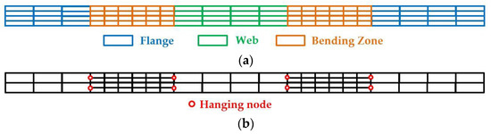
Figure 1.
Example of a non-conformal mesh applied to the transverse section of a roll-formed sheet. Initial undeformed configuration. (a) Classic conformal FE mesh; (b) Non-conformal FE mesh. In both cases, the regions where bending will take place need to have a larger number of elements through the thickness.
The main drawback of using non-conformal meshes is the handling of “hanging nodes”, which are non-matching nodes at the interfaces between the fine and coarse regions. The literature includes three main categories of methods to deal with hanging nodes. The first one consists in addressing the discontinuity introduced by the hanging nodes by using a discontinuous finite element formulation (e.g., discontinuous Galerkin [23,24,25]). While those methods are effective, changing the formulation can be impractical in an already established finite element code. The second category keeps a continuous formulation but imposes constraints on the hanging nodes to enforce the continuity of the solution. This is usually done by removing the degrees of freedom of the hanging nodes and imposing them in a post-computation step (e.g., condensation and recovery method [26,27]). This second category is the most common in the literature and has proven its effectiveness. However, its implementation requires advanced algorithmic treatment. Moreover, some limitations are usually imposed on the created meshes for ease of implementation. The most common limitation is not to allow constrained nodes to be part of multiple constraints (e.g., limitation to “one-irregular” mesh according to [27]). The third category of methods also keeps a continuous formulation but maintains the continuity throughout the computation with enrichments to the formulation (e.g., expanded shape function support [28,29], and hanging nodes handled by Lagrange Multipliers [30,31]). Contrary to the second category, no restrictions on the number of constraints on each node are required, making the methods more flexible in the type of meshes that can be created.
In this work, the third category of methods is used by adding a constraint on the hanging nodes using Lagrange Multipliers. Similar developments can be observed in [30] in the scope of geomechanics and in [31] applied to eXtended Finite Element Method simulations. While the use of Lagrange Multipliers has the drawback of adding degrees of freedom to the problem, the generality of the approach allows for a very easy and swift definition of a wide variety of non-conformal meshes. The present work will highlight the ease of use and implementation of this method in an implicit FE software combined with its novel application to roll-forming simulations.
This work is the continuation of previous work done by the authors on roll-forming simulations [1,2,3,4] using the in-house implicit non-linear finite element solver Metafor [32,33] developed at the University of Liège. In previous publications, the ALE method was adopted in an attempt to tackle the issue of high computational costs obtained with traditional Lagrangian models. While the ALE method could reproduce the results obtained with a Lagrangian approach and is arguably better suited to model continuous roll-forming processes, the CPU time remained excessively high. The present paper takes the first step towards implementing non-conformal meshes to simulate roll forming using Metafor [32,33]. This work will initially be limited to a Lagrangian model, and further developments will be needed to apply the proposed method to ALE models.
The paper is structured as follows: Section 2 shows the details of the implementation of hanging nodes using Lagrange Multipliers. Section 3 shows increasingly complex simulations using non-conformal meshes, including complex roll forming (forming of a U-channel and tubular rocker panel). Section 4 presents the conclusions that can be drawn from this work.
2. Method: Lagrange Multipliers and Hanging Nodes
The main feature of non-conformal meshes is the presence of hanging nodes, which require specific treatment. Indeed, the finite element method assumes the continuity of the displacement field all over the mesh. However, this continuity is usually satisfied thanks to node sharing between adjacent finite elements. This does not hold true with non-conformal meshes since there is no more guarantee that adjacent elements will share the same nodes. As such, Figure 2 illustrates a possible discontinuous displacement between 2 adjacent elements that can arise from the presence of hanging nodes if they are not handled. To fix this issue, the position of each of them needs to be imposed with regard to its neighbors. The proposed method consists in using Lagrange Multipliers to impose this constraint.
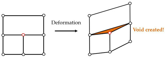
Figure 2.
Examples of possible discontinuous displacements that occur if a hanging node (in red) is not correctly handled.
The constraint to be imposed on a single hanging node is such that its relative position to the boundary of its neighbor element remains constant. Examples of such constraints can be observed in Figure 3 for the connection of 5 hanging nodes to the 2D bilinear boundary of a 3D trilinear hexahedral element. The general formulation of the constraints reads:
where represents the total number of hanging nodes, is the position vector of the hanging node, is the position vector of the node of the neighbor element and is its associated shape function evaluated at the reduced isoparametric coordinates of the hanging node on the boundary of the neighbor element. is the number of nodes of this boundary (e.g., 2 for a 1D linear boundary, 4 for a 2D bilinear boundary). This constraint ensures that the position of the hanging node will remain at the same reduced isoparametric coordinates () with respect to the boundary of the neighbor element. This work is currently limited to linear elements.
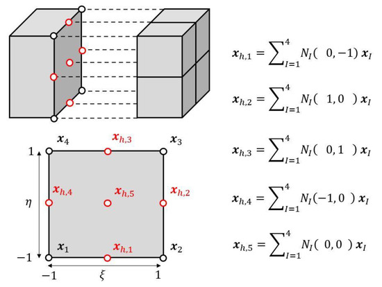
Figure 3.
Example of constraint relations obtained in the case of 5 hanging nodes ( to in red) connected to a 2D bilinear quadrangle boundary. Note that the general formulation has been used but some of the shape functions are null. (e.g., in the expression for node ).
Note that for each hanging node, one constraint is created per dimension of the system, resulting in a total number of constraints of ( in 2D, in 3D). For the sake of simplifying the notation, the constraints are hereafter considered component by component without loss of generality:
where represent one component of .
To understand how the constraints are handled in Metafor [32,33], one must first understand how the classical conformal FE problem is solved. As a starting point, the generalized position vector at time can be written as the sum of its value at the previous time and an increment during the time step :
where:
where is the total number of unknowns (from hanging and non-hanging nodes).
For the pure conformal case, obtaining the solution at time from the solution at time means finding the that will keep the body in equilibrium at time . At each time step, an estimate for is obtained using an iterative Newton–Raphson scheme. The equations to solve between each time step involve setting to zero the norm of the non-linear out-of-balance forces
where and respectively represent the internal and external forces associated with the generalized position vector . Through classical FEA developments, is approximated by the following first-order Taylor expansion:
or
where is the Newton–Raphson iteration counter, is the current estimate of is the iterative correction on and is the tangent stiffness matrix defined as:
As we want in (7), the new estimate for is thus given by:
The procedure is repeated until we obtain a sufficient precision on (5), e.g., using:
where is a user-defined tolerance on the norm of with a default value of .
On top of the above procedure, for the non-conformal case, the treatment of the hanging nodes requires enforcement of the constraints defined in (2). Following Belytschko et al. [34], imposing such constraint using the Lagrange Multiplier method leads to adding the following additional forces associated to each constraint :
where is one constraint on one hanging node (see (2)) and represents its associated Lagrange Multiplier. For each hanging node, one constraint and one degree of freedom are added per dimension of the system (2 in 2D, 3 in 3D) By analogy with (3) the newly added Lagrange Multiplier can be written as the sum of its value at the previous time and its increment for the current time step :
Combining Equation (5) with the additional forces associated with the constraints (11), one obtains a new force to set to zero defined as:
Following Belytschko et al. [34], equation (14) is approximated by a first-order Taylor expansion in both and and its result is set to zero ( is the current Newton-Raphson estimate of is its current iterative correction):
Then, if we define:
we obtain:
where and respectively represent vectors containing the added Lagrange Multipliers and their associated iterative correction . If linear constraints are used, as it is the case here, we have
The constraints from (2) also need to be satisfied. Approximating each by a first order Taylor expansion and setting the results to zero yields:
Writing the constraints in matrix form results in defined as:
we then obtain the following expression for (18):
The linear model resulting from (17) and (20) can be put in matrix form given by:
where is the same tangent stiffness matrix as for the conformal case. The new estimates of and are then given by:
Similarly, as for the conformal case, the procedure is repeated until sufficient precision is obtained on (13), e.g., using:
Note that this development was done using a quasi-static assumption, but the same procedure is also applicable for dynamic problems leading to similar linearized equations [34].
The practical impact of the Lagrange Multipliers on the finite element simulation is that forces are added to the system of equations such that the Newton–Raphson iterative solution naturally fulfills the constraint (see Figure 4).
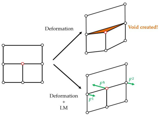
Figure 4.
Forces generated by the Lagrange Multipliers .
3. Results and Discussion
In this section, the proposed hanging node implementation is assessed with progressively more complex simulations. The correct implementation of the hanging nodes is first verified with a simple geometry, a cube submitted to simple shear. Then, a more complex 2D simulation of the flanging of a metal sheet is conducted, including spring back. Afterward, the first application of 3D roll forming of a U-channel is discussed and compared to numerical and experimental results as proof of the usefulness of the proposed method applied to roll forming simulations. Finally, the results of a more complex application are discussed, assessing the use of the proposed method for industrial purposes (forming of a tubular rocker panel).
3.1. 2D Verification Tests
3.1.1. Cube Submitted to Simple Shear
As an indication of the good behavior of the implementation of the constraints at the hanging nodes in Metafor [32,33], a simple 2D test consisting of a elastic cube (Young’s modulus , Poisson’s ratio ) undergoing simple shear is hereafter shown. A state of plane strain assumption is made. To take into account large deformations, a hypoelastic model is considered, associated with a Jaumann objective derivative [33]. The mesh, as well as the boundary conditions, can be observed in Figure 5. The test is displacement driven with and one single time step is used. In this case, the boundary conditions have been chosen so that the vertical displacement of the hanging node is the only free unknown of the system. This will allow a good insight into the correct behavior of the Lagrange Multipliers to handle the hanging node.
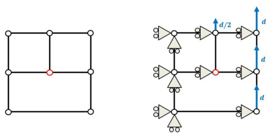
Figure 5.
Mesh (left) and boundary conditions (right) for a elastic cube submitted to simple shear using a non-conformal mesh. Plane strain assumption. The imposed displacements are represented by blue arrows with . One single time step.
The impact of the Lagrange Multiplier on the vertical displacement of the hanging node can be observed in Figure 6. The displacement is clearly discontinuous at the hanging node in the case where no constraint has been applied, an overlap of finite elements can be observed. The displacement is, however, perfectly continuous when the hanging node is managed by the method. The results are as can be expected for an elastic cube submitted to simple shear; one can indeed see a perfectly linear solution for the vertical displacement. In the case including Lagrange Multipliers, Figure 7 shows the expected results of a constant in-plane shear component (XY) of the Cauchy stress tensor. Overall, the method gives correct results for this simple case.
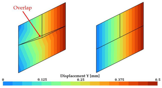
Figure 6.
2D simulation of a cube submitted to simple shear, vertical displacement. (left): no Lagrange Multiplier; (right) Lagrange Multiplier.
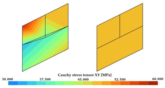
Figure 7.
A 2D simulation of a simple submitted to pure shear, in-plane shear (XY) component of the Cauchy stress tensor. (left): no Lagrange Multiplier; (right) Lagrange Multiplier.
3.1.2. 2D Flanging of a Metal Sheet
The proposed method is applied to a 2D flanging simulation as proof of the usefulness of the method in the scope of bending operations. The principle of the process can be observed in Figure 8. The sheet thickness is . The radii of the sheet holder, die, and punch are respectively , and . The width of the sheet holder, die, and punch are respectively , and . The distance between the sheet holder and the punch is .
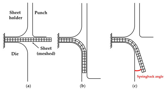
Figure 8.
Principle of the 2D flanging process, meshed sheet, rigid tools. (a) Initial configuration; (b) Imposed shape after maximum punch displacement of ; (c) Shape after spring back.
This test consists in the flanging of a steel sheet. The evolution of the process over time is shown in Figure 9. It is as follows: first at the sheet is fitted between the die and the sheet holder. The punch is placed right against the sheet. From to the punch moves downwards and bends the sheet up to a 90° angle. The punch then keeps moving downwards until t = 10.0 s (maximal displacement = 20 mm). At t = 10.0 s, the punch then starts going back upward towards its original position. The spring back of the sheet occurs between t = 16.0 s and t = 18.0 s.
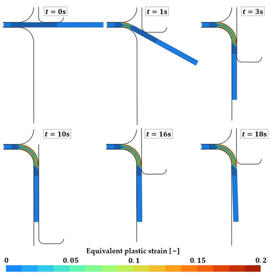
Figure 9.
A 2D flanging simulation in Metafor [32,33]. Evolution of the process over time.
The simulation is performed with a state of plane strain assumption. Values of 210 GPa and 0.3 have been chosen for the Young’s modulus and Poisson’s ratio. The sheet is modeled with a linear isotropic hardening, the initial yield strength and the hardening coefficient are taken at 396 MPa and 1495 MPa, respectively.
The leftmost part of the sheet is clamped. A frictionless contact is used between the sheet and the die, the punch, and the blank holder. The contact is modelled by a penalty method. The forming angle and the amplitude of the resultant force applied by the punch are compared between simulations using seven different finite element meshes using four-noded bilinear quadrangular elements. Both conformal and non-conformal meshes are considered (Figure 10). A four Gauss point quadrature rule is used for spatial integration of the element. To avoid locking, a constant pressure element is used (Q4P0).
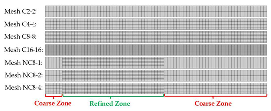
Figure 10.
A 2D flanging simulation, seven different finite element meshes, conformal (C) or non-conformal (NC) with a varying number of elements through the thickness (see Table 1 for number of elements).
The name and number of elements associated with each of the created meshes are available in Table 1. Three different non-conformal meshes have been created with 1, 2, or 4 elements though the thickness in the coarse regions () and 8 elements through the thickness in the refined region (), where the bending will mainly occur (green region in Figure 10). As a reference, four different conformal meshes have been created with a varying number of elements (2, 4, 8, 16) through the full sheet thickness.

Table 1.
A 2D flanging simulation. Number of elements and computation time (on one Intel Core i7-9750H 2.6 GHz processor) for the seven different FE meshes. and , respectively, represents the number of elements through the thickness in the refined zone and in the coarse zone (see Figure 10).
The impact of the number of finite elements through the sheet thickness on the angle between the sheet and the die is depicted in Figure 11a,b using only conformal meshes. The spring back can be observed in Figure 11b. Those tests indicate that 8 elements are required through the thickness for a good convergence of the angle after spring back. The same conclusion can be made by observing the resultant force applied by the punch (Figure 11c,d). Indeed, a noticeable difference is observed for meshes with only 2 or 4 elements through the thickness (C2-2 and C4-4), while almost no difference can be observed for the meshes having 8 or 16 elements through the thickness (C8-8 and C16-16). The oscillations observed in the punch force (Figure 11c,d) are present due to the rather coarse discretization in the longitudinal direction and more elements should be used if a more accurate representation of the physical process is required. The current study, however, focuses on the verification of the results between different meshes and as such this longitudinal discretization is deemed sufficient. The optimal number of elements through the thickness for a good accuracy of the results thus seems to be 8 and mesh C8-8 will now be considered as the reference mesh for future comparisons.
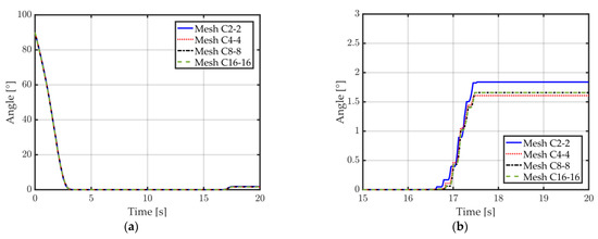
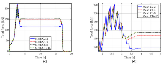
Figure 11.
A 2D flanging simulation, conformal meshes C2-2, C4-4, C8-8, and C16-16 (see Table 1 for mesh details). (a) Angle between sheet and die over time; (b) Zoom on the angle (visible spring back); (c) Total force applied by the punch over time; (d) Zoom on the total force (during bending).
Likewise, the angle after spring back also converges to the same value for all tested non-conformal meshes and no significant differences can be observed (Figure 12a,b). The resultant force applied by the punch is almost undistinguishable between the reference mesh and the non-conformal meshes for the first 3.0 s of the process, where most of the sheet deformation takes place. After the first 3.0 s, a slight difference can be observed for Mesh NC8-1 while the other meshes keep equal results (Figure 12c,d). Overall, the results using non-conformal meshes show little to no impact on the accuracy of the model compared to the reference mesh C8-8.
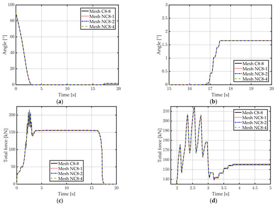
Figure 12.
A 2D flanging simulation, meshes NC8-1, NC8-2, and NC8-4 are compared to conformal mesh C8-8 (see Table 1 for mesh details). (a) Angle between sheet and die over time; (b) Zoom on the angle (visible spring back); (c) Total force applied by the punch over time; (d) Zoom on the total force (during bending).
The computation time for the seven different meshes are shown in Table 1. The simulations using non-conformal meshes reveal that one can obtain coarser FE meshes, resulting in overall less costly models, with a negligible impact on the accuracy. It should be noted that although the gains obtained in this rather small 2D test are already promising (~43% CPU gain for similar accuracy between mesh C8-8 and NC8-1), the potential gains in computational time are expected to be greater when expanding those results to 3D simulations. Although the use of Lagrange Multipliers to impose the constraints on the hanging nodes added degrees of freedom to the problem, the method allowed a substantial reduction in mesh sizes.
3.2. 3D Roll Forming Applications
3.2.1. Forming of a U-Channel
We consider here the case of the forming of a symmetric U-channel described in [2] (width , thickness , bending radius ) where the mill features six forming stands with the following sequence of forming angles: 15°, 32°, 50°, 68°, 80°, and 90°. The model contains an additional purely numerical 0° stand to help drive the sheet through friction. The distance between two consecutive stands is . The length of the sheet is chosen equal to . The forming velocity is and the friction coefficient µ between the rolls and the sheet is equal to 0.2. The rolls are assumed to be perfectly rigid, and the contact is modelled by a penalty method.
The progress of a roll-forming simulation in Metafor [32,33] is as follows [2,3,4]: initially, the sheet is positioned in front of the roll-forming mill (Figure 13). A prescribed displacement is applied to the front and rear sides of the sheet until friction with the rotating rolls becomes sufficient to drive the sheet in the forming direction. Similarly, additional boundary conditions are used when releasing the sheet from the last two forming stands. See [2,3,4] for further details.
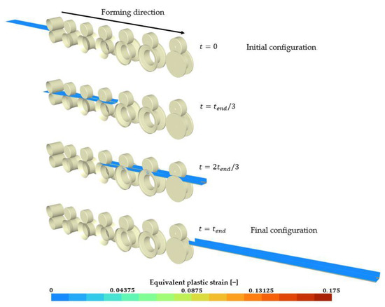
Figure 13.
Roll-forming simulation in Metafor [32,33] in the case of the forming of a U-Channel discussed in [2,3,4], (sheet length = and inter-stand distance ).
The material used for all roll-forming simulations in this work is a high-strength DP980 steel, with Young’s modulus and Poisson’s ratio . An isotropic hardening model is considered using the following Swift law:
The constitutive material behavior has been studied extensively [35,36] in the scope of this particular forming mill. Previous studies suggest that the kinematic hardening may be safely neglected since no plastic unbending occurs during the forming process [1].
Measurements such as the forming angle and the final shape of the sheet are all analyzed in the middle section of the sheet (white line in Figure 14). This section is the most representative of a continuous forming process since it is the furthest away from both front and rear ends of the sheet, thus mitigating the impact of edge effects as well as reducing the influence of boundary conditions. The final shape, after spring back, will be compared to experimental data coming from [2] where the shape of the experimental 2000 mm long U-channel has been digitized outside the mill by a 3D high-precision measurement device. Moreover, the vertical displacement of the middle point (red dot in Figure 14) throughout the simulation will also be studied and compared to experimental measurements collected with a portable arm equipped with a contact-sensing rigid probe. Note that measurements are only available on the upper surface of the sheet, but numerical results will be given for both upper and lower surfaces. Lastly, longitudinal Green–Lagrange strains are computed at the middle point and on the left edge of the measurement section (red and purple dots in Figure 14).
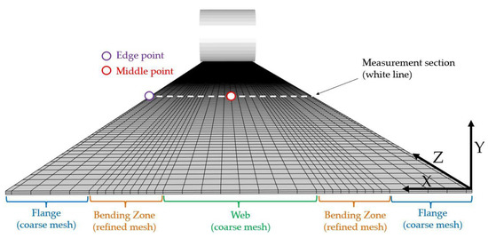
Figure 14.
Example of conformal mesh for the forming of a U-channel. Initial state.
Figure 14 shows a typical conformal mesh where a more refined discretization is chosen along the transversal direction within each bending zone while the flange and web are more coarsely meshed. The size of the bending regions is chosen with the help of the final geometry of the flower diagram coming from the roll-design software COPRA RF [37]. A value of was taken for each bending region in this example. One can note that the process is such that the bending zones stay at a similar transverse location throughout the full process length, allowing an easy definition of efficient non-conformal meshes.
Three different conformal meshes and three different non-conformal meshes with a varying number of elements through the sheet thickness are first created (Figure 15). Enhanced Assumed Strain (EAS) elements, where additional internal deformation modes are introduced in the strain field of elements [38,39,40], are chosen. Previous study [39] suggests that EAS elements allow for a reliable modeling of the spring back of metal sheets with a coarser mesh than standard locking-free finite elements. Moreover, this choice of elements demonstrates that the hanging node implementation is not limited to a particular type of element. The number of elements and the computation time for each mesh are available in Table 2. The final state of the simulation can be observed in Figure 16 for two of the proposed meshes.
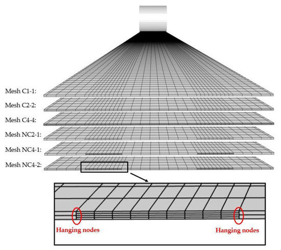
Figure 15.
Forming of a U-Channel. Three conformal meshes and three non-conformal meshes with a varying number of elements through the sheet thickness (see Table 2 for number of elements).
Table 2.
Forming of a U-Channel. Number of elements and computation time (on two 6-core Intel Xeon X5650 2.67 GHz processors, giving 12 cores in total) for the 6 different finite element meshes. and respectively represents the number of elements through the thickness in the refined zone (bending zone) and in the coarse zone (flange + web).
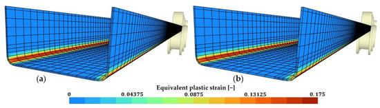
Figure 16.
Final state of the simulation. (a) Conformal mesh C2-2; (b) Non-conformal mesh NC2-1.
Results for the three reference conformal meshes (C1-1, C2-2, C4-4) are available in Figure 17a–f. The influence of the mesh on the final shape of the U-channel after spring back is illustrated in Figure 17a, where mesh C1-1 reveals that having too few elements through the thickness of the sheet can lead to inaccuracies of the final U shape. Mesh C2-2 and C4-4 both agree well with the experimental shape of the measurement section (Figure 17a) as well as to the vertical displacement of the middle point of the measurement section (Figure 17b). Minor differences are noticeable between the results of mesh C2-2 and C4-4. These differences are more visible when looking at the forming angle during the course of the process where a difference of about 0.4° can be observed for the final forming angle after spring back (Figure 17c,d). The evolution of the longitudinal Green–Lagrange strain on two different points of the measurement section can be visualized in Figure 17e,f. All three meshes give relatively similar results, although mesh C1-1 is again noticeably apart from the other two.
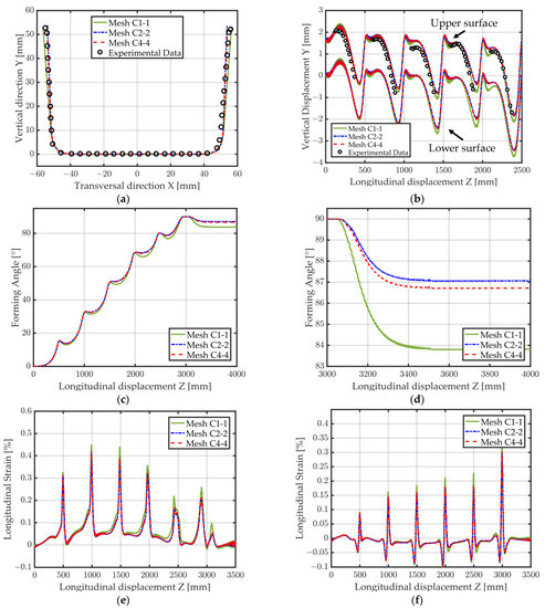
Figure 17.
Forming of a U-Channel. Simulation results for the three conformal meshes C1-1, C2-2, C4-4 (see Table 2 for mesh details). (a) Final shape; (b) Vertical displacement at middle point location (red dot in Figure 14), upper and lower surfaces; (c) Forming angle; (d) Zoom on the forming angle (visible spring back); (e) Longitudinal Green–Lagrange strain (edge point); (f) Longitudinal Green–Lagrange strain (middle point).
The main conclusion of the results obtained with conformal meshes is that using only one element in the thickness (mesh C1-1) is not sufficient to accurately capture the bending of the sheet during the process which leads to overall inaccurate results. Using four elements instead of two elements through the thickness is, however, debatable since the difference in the results is minimal. The increase in computational time going from mesh C2-2 to mesh C4-4 is extremely high (+140% CPU). The best compromise between accuracy and computational time appears to be mesh C2-2 if only conformal meshes are used. The use of EAS elements might explain the very accurate results obtained with as few as two elements in the sheet thickness.
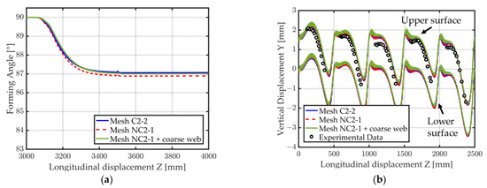
Figure 18 compares the results obtained with non-conformal mesh NC2-1 with the results obtained with conformal mesh C2-2. The final U-shape, the vertical displacement and longitudinal Green–Lagrange strain over the process (Figure 18a,b,e,f) are almost indistinguishable between mesh C2-2 and NC2-1. The final forming angle after spring back is illustrated in Figure 18c,d and only differs by about 0.1° between the two meshes. Overall, the impact of using this non-conformal mesh on the final accuracy of the results is quite negligible. Moreover, a 37% decrease in computational time was observed between the simulations using mesh C2-2 and mesh NC2-1.
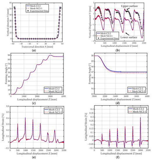
Figure 18.
Forming of a U-Channel. Simulation results for meshes C2-2, NC2-1 (see Table 2 for mesh details). (a) Final shape; (b) Vertical displacement at middle point location (red dot in Figure 14), upper and lower surfaces; (c) Forming angle; (d) Zoom on the forming angle (visible spring back); (e) Longitudinal Green–Lagrange strain (edge point); (f) Longitudinal Green–Lagrange strain (middle point).
Other non-conformal meshes containing more elements in the refined region were also investigated (mesh NC4-1 and NC4-2 in Figure 15). The forming angles using those meshes are compared to mesh C2-2 and C4-4 in Figure 19a. Both non-conformal meshes perform extremely well with a final difference in forming angle of only about 0.1° with respect to mesh C4-4. Looking at the computational time (Table 2), it is obvious that if four elements are to be used in the refined region, the non-conformal meshes can lead to significantly reduced CPU time (going from 24 h 21 m for mesh C4-4 down to 10 h 58 m for mesh NC4-1). Furthermore, the impact on the accuracy compared to the full conformal mesh C4-4 is minimal. Non-conformal mesh NC4-1 is still noticeably more costly than mesh C2-2, and is only computationally interesting with respect to the full mesh C4-4. However, mesh NC2-1 is much cheaper than mesh C2-2.
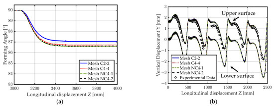
So far, only the number of elements through the thickness was considered for the coarsening. Figure 20 highlights the flexibility in mesh creation allowed by the proposed method by creating a new NC2-1 mesh where the web has also been coarsened in the longitudinal direction. Figure 21a shows that a good agreement for the forming angle is obtained compared to mesh C2-2 (less than 0.1° difference). It can be noted that in this particular example, coarsening the mesh in the thickness tends to underestimate the final angle while coarsening the web in the longitudinal direction tends to overestimate the final angle, this leads to the result obtained here where mesh “NC2-1 + coarse web“ is closer to the results of mesh C2-2 than mesh NC2-1. However, the vertical displacement of the middle measurement point shows inaccuracies for the coarser mesh (Figure 21b). Such discretization may thus be used as a first step to quickly assess the final shape of the cross-section but if detailed results are required along the longitudinal direction this type of mesh coarsening might need to be avoided. Nevertheless, the creation of this mesh was possible thanks to the proposed method and a computational time of 4 h 51 m could be obtained. This allowed for an even faster computational time compared to mesh NC2-1 (6 h 27 m) with a slight degradation of the accuracy of some results (Figure 21b), while the accuracy on the final forming angle remained acceptable (Figure 21a).
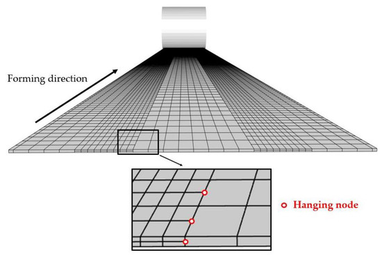
Figure 20.
Forming of a U-Channel. Non-conformal mesh “NC2-1 + coarse web along the forming direction”.
3.2.2. Forming of a Tubular Rocker Panel
A similar analysis has been carried out for the forming of a tubular rocker panel; this section will present the most relevant results without going into as much detail as in Section 3.2.1. This application was studied in depth using the ALE formalism in previous work [2,3,4]. The test consists of the forming of a non-symmetric tubular rocker panel (initial dimensions: width , thickness ). The forming mill is a real industrial continuous roll-forming line consisting of 16 stands with an inter-stand distance of . The total sheet length is . Figure 22 shows the full forming line as well as its related flower diagram. In contrast with [4], no welding operation is conducted in this work, this will create a more noticeable spring back. Contrary to the U-channel, frictionless contact is assumed. The sheet has a zero prescribed longitudinal displacement on its rear and front section, and it is the tools that are moved along the sheet. This procedure is a simplification of the traditional simulations shown in Section 3.2.1. The rolling tools are considered rigid, the contact between the rolls and the sheet is modeled by the penalty method. The same material model as for the U-channel is used. The final shape of the cross-section as well as the vertical displacement and longitudinal Green–Lagrange strain will be compared between different finite element meshes. Similarly, as for the U-channel, all results are computed at a measurement section situated on the middle of the sheet in the longitudinal direction.
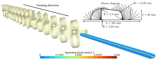
Figure 22.
Forming of a tubular rocker panel, final state. 16-stand forming line and flower diagram.
The two meshes are depicted in Figure 23 in their initial configuration and in Figure 24 in the final state of the simulation. The reference mesh is conformal, has four elements through the sheet thickness and a constant element size of 3 mm along the longitudinal direction. In the transversal direction, each bending zone contains seven elements, each other zone has an element size of around 6 mm. The optimized mesh has the same discretization in the transversal direction. However, following results from Section 3.2.1, the mesh is made non-conformal by reducing the number of elements through the thickness to two for the flange and web zones (see Figure 23). Coarsening is also carried out in the longitudinal direction by dividing the number of elements in the web zones by 2. The number of elements in the flange zones is, however, maintained since a poor entry into the second mill was obtained by coarsening the mesh in those regions. This once again shows the versatility of the approach in creating FE meshes tailored to the specific process and geometry. Table 3 contains the CPU time as well as the number of elements and number of hanging nodes used.
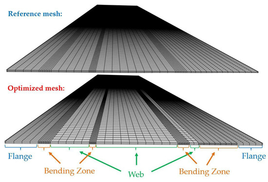
Figure 23.
Forming of a tubular rocker panel, initial state. Reference conformal mesh and optimized non-conformal mesh.
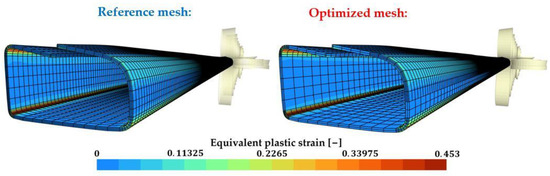
Figure 24.
Forming of a tubular rocker panel, final state. Reference conformal mesh and optimized non-conformal mesh.
Table 3.
Forming of a tubular rocker panel. Number of elements, number of hanging nodes and computation time (on two 6-core Intel Xeon X5650 2.67 GHz processors, giving 12 cores in total) for the reference mesh and the optimized mesh.
The longitudinal Green–Lagrange strains as well as the vertical displacement of a point situated on the left edge of the measurement section and of a point located on the middle of the measurement section can be observed in Figure 25a–d. All curves show a very good agreement between the reference mesh and the optimized non-conformal mesh. A good agreement between the shapes of the two cross-sections is observed. Table 3 shows that going from the reference mesh to the optimized non-conformal mesh significantly reduces the computational time (from 2 d 15 h 9 m to 1 d 6 h 33 m). Hence, the proposed optimized mesh allows a sizable cost decrease (51.6%) with a negligible impact on the shape of the final cross-section.
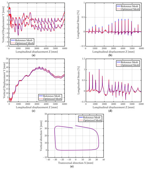
Figure 25.
Forming of a tubular rocker panel. Simulation results for both meshes. (a) Vertical displacement (middle); (b) Longitudinal Green–Lagrange strain (middle); (c) Vertical displacement (left edge); (d) Longitudinal Green–Lagrange strain (left edge); (e) Final shape.
4. Conclusions
This work had the goal of improving the computational efficiency of finite element simulations of roll-forming processes by introducing non-conformal meshes where hanging nodes are handled by Lagrange Multipliers. The implementation of the method was first verified with 2D simulations of a cube submitted to simple shear and of the flanging of a metal sheet. Valid results were obtained for simulations using non-conformal meshes. The method was then applied to the forming of a U-channel where the influence of non-conformal meshes on the accuracy and computational time was discussed. The proposed method offers the possibility to create coarser FE meshes, resulting in overall smaller computational cost, with little to no impact on the accuracy of the results. As for any finite element mesh, it is, however, still important to check for the convergence of the mesh since excessive or ill-placed coarsening of the mesh could lead to erroneous results. Finally, as proof of the industrial applicability of the method, it was used on the forming of a non-symmetric tubular rocker panel. A mesh specifically tailored to this complex roll forming mill could easily be created using non-conformal meshes. This led to a substantial gain in computational time (51.6% reduction on a 2 d 15 h 9 m simulation) with a negligible impact on the results. The method can thus easily be used to create lighter meshes for roll-forming applications. Nevertheless, the current study presents some limitations. First, linear elements were used due to the easier implementation of linear Lagrange Multiplier constraints, the extension to higher order elements should, however, lead to similar conclusions and is a possible future prospect. Moreover, no comparison to other non-conformal mesh methods or software has been conducted; the present study only planned on highlighting the usefulness of non-conformal meshes applied to roll-forming simulation in an effective and easy manner. In addition, both shown roll-forming simulations have deformation zones which remain at a similar location along the sheet transverse direction throughout the full process; this allowed for an easier definition of the optimized non-conformal meshes. More complex roll-forming processes where the deformation zones move over the full sheet throughout the process would require additional numerical techniques to take advantage of the method. The ALE formalism or dynamic re-meshing schemes combined with non-conformal meshes could be a good prospect for future work on this issue. Finally, the reader may note that more optimized meshes can likely be created for an even better reduction of the computational cost.
Author Contributions
Conceptualization, C.L.; Formal analysis, C.L., R.B., L.P., and J.-P.P.; Methodology, C.L.; Software, C.L., R.B., and L.P.; Supervision, J.-P.P.; Validation, C.L.; Writing—original draft, C.L.; Writing—review & editing, R.B., L.P., and J.-P.P. All authors have read and agreed to the published version of the manuscript.
Funding
This research received no external funding.
Data Availability Statement
Any requirement about the data of this research must be consulted directly with the corresponding author.
Conflicts of Interest
The authors declare no conflict of interest.
References
- Viet, B.Q.; Boman, R.; Papeleux, L.; Wouters, P.; Kergen, R.; Daolio, G.; Duroux, P.; Flores, P.; Habraken, A.; Ponthot, J.-P. Springback and twist prediction of roll formed parts. In Proceedings of the IDDRG 2006 International Deep Drawing Research Group, Drawing the Things to Come, Trends and Advances in Sheet Metal Forming, Porto, Portugal, 19–21 June 2006. [Google Scholar]
- Boman, R.; Ponthot, J.P. Continuous roll forming simulation using arbitrary Lagrangian Eulerian formalism. Key Eng. Mater. 2011, 473, 564–571. [Google Scholar] [CrossRef]
- Crutzen, Y.; Boman, R.; Papeleux, L.; Ponthot, J.-P. Lagrangian and arbitrary Lagrangian Eulerian simulations of complex roll-forming processes. Comptes Rendus Mec. 2016, 344, 251–266. [Google Scholar] [CrossRef]
- Crutzen, Y.; Boman, R.; Papeleux, L.; Ponthot, J.-P. Continuous roll forming including in-line welding and post-cut within an ALE formalism. Finite Elem. Anal. Des. 2018, 143, 11–31. [Google Scholar] [CrossRef]
- Yan, Y.; Wang, H.; Li, Q.; Guan, Y. Finite element simulation of flexible roll forming with supplemented material data and the experimental verification. Chin. J. Mech. Eng. 2016, 29, 342–350. [Google Scholar] [CrossRef]
- Tsang, K.S.; Ion, W.; Blackwell, P.; English, M. Validation of a finite element model of the cold roll forming process on the basis of 3D geometric accuracy. Proc. Eng. 2017, 207, 1278–1283. [Google Scholar] [CrossRef]
- Lun, F.; Li, R.; Li, M.; Qiu, N.; Xue, P. Forming load in flexible rolling process for sheet metal parts. Int. J. Adv. Manuf. Technol. 2015, 77, 1333–1344. [Google Scholar] [CrossRef]
- Joo, B.; Lee, H.; Kim, D.; Moon, Y. A study on forming characteristics of roll forming process with high strength steel. AIP Conf. Proc. 2011, 1383, 1034–1040. [Google Scholar] [CrossRef]
- Falsafi, J.; Demirci, E.; Silberschmidt, V. Numerical study of strain-rate effect in cold rolls forming of steel. J. Phys. Conf. Ser. 2013, 451, 012041. [Google Scholar] [CrossRef]
- Kasaei, M.M.; Moslemi Naeini, H.; Abbaszadeh, B.; Roohi, A.H.; Silva, M.B.; Martins, P.A. On the prediction of wrinkling in flexible roll forming. Int. J. Adv. Manuf. Technol. 2021, 113, 2257–2275. [Google Scholar] [CrossRef]
- Mohammdi Najafabadi, H.; Moslemi Naeini, H.; Safdarian, R.; Kasaei, M.; Akbari, D.; Abbaszadeh, B. Effect of forming parameters on edge wrinkling in cold roll forming of wide profiles. Int. J. Adv. Manuf. Technol. 2019, 101, 181–194. [Google Scholar] [CrossRef]
- Tajik, Y.; Naeini, H.M.; Tafti, R.A.; Bidabadi, B.S. A strategy to reduce the twist defect in roll-formed asymmetrical-channel sections. Thin-Walled Struct. 2018, 130, 395–404. [Google Scholar] [CrossRef]
- Li, K.; Carden, W.; Wagoner, R. Simulation of springback. Int. J. Mech. Sci. 2002, 44, 103–122. [Google Scholar] [CrossRef]
- Ghiabakloo, H.; Kim, J.; Kang, B.-S. An efficient finite element approach for shape prediction in flexibly-reconfigurable roll forming process. Int. J. Mech. Sci. 2018, 142, 339–358. [Google Scholar] [CrossRef]
- Görtan, M.O.; Vucic, D.; Groche, P.; Livatyali, H. Roll forming of branched profiles. J. Mater. Process. Technol. 2009, 209, 5837–5844. [Google Scholar] [CrossRef]
- Groche, P.; Mueller, C.; Traub, T.; Butterweck, K. Experimental and numerical determination of roll forming loads. Steel Res. Int. 2014, 85, 112–122. [Google Scholar] [CrossRef]
- Luo, Z.; Sun, M.; Zhang, Z.; Lu, C.; Zhang, G.; Fan, X. Finite element analysis of circle-to-rectangle roll forming of thick-walled rectangular tubes with small rounded corners. Int. J. Mater. Form. 2022, 15, 73. [Google Scholar] [CrossRef]
- Essa, A.; Abeyrathna, B.; Rolfe, B.; Weiss, M. Prototyping of straight section components using incremental shape rolling. Int. J. Adv. Manuf. Technol. 2022, 121, 3883–3901. [Google Scholar] [CrossRef]
- Min, J.; Wang, J.; Lian, J.; Liu, Y.; Hou, Z. Laser-Assisted Robotic Roller Forming of Ultrahigh-Strength Steel QP1180 with High Precision. Materials 2023, 16, 1026. [Google Scholar] [CrossRef]
- Liang, C.; Li, S.; Liang, J.; Li, J. Method for Controlling Edge Wave Defects of Parts during Roll Forming of High-Strength Steel. Metals 2022, 12, 53. [Google Scholar] [CrossRef]
- Wang, J.; Liu, H.-M.; Li, S.-F.; Chen, W.-J. Cold Roll Forming Process Design for Complex Stainless-Steel Section Based on COPRA and Orthogonal Experiment. Materials 2022, 15, 8023. [Google Scholar] [CrossRef]
- Xing, M.; Wang, H.; Liu, J.; Fu, Y.; Du, F. Application of Mean Modulus in Three-Point Bending and Roll Forming. Materials 2023, 16, 2571. [Google Scholar] [CrossRef]
- Badia, S.; Baiges, J. Adaptive finite element simulation of incompressible flows by hybrid continuous-discontinuous Galerkin formulations. SIAM J. Sci. Comput. 2013, 35, A491–A516. [Google Scholar] [CrossRef]
- Houston, P.; Schötzau, D.; Wihler, T.P. An hp-adaptive mixed discontinuous Galerkin FEM for nearly incompressible linear elasticity. Comput. Methods Appl. Mech. Eng. 2006, 195, 3224–3246. [Google Scholar] [CrossRef]
- Cockburn, B.; Kanschat, G.; Schötzau, D.; Schwab, C. Local discontinuous Galerkin methods for the Stokes system. SIAM J. Numer. Anal. 2002, 40, 319–343. [Google Scholar] [CrossRef]
- Baiges, J.; Bayona, C. Refficientlib: An Efficient Load-Rebalanced Adaptive Mesh Refinement Algorithm for High-Performance Computational Physics Meshes. SIAM J. Sci. Comput. 2017, 39, C65–C95. [Google Scholar] [CrossRef]
- Bangerth, W.; Hartmann, R.; Kanschat, G. deal. II—A general-purpose object-oriented finite element library. ACM Trans. Math. Softw. TOMS 2007, 33, 24-es. [Google Scholar] [CrossRef]
- Zander, N.; Bog, T.; Kollmannsberger, S.; Schillinger, D.; Rank, E. Multi-level hp-adaptivity: High-order mesh adaptivity without the difficulties of constraining hanging nodes. Comput. Mech. 2015, 55, 499–517. [Google Scholar] [CrossRef]
- Di Stolfo, P.; Schröder, A.; Zander, N.; Kollmannsberger, S. An easy treatment of hanging nodes in hp-finite elements. Finite Elem. Anal. Des. 2016, 121, 101–117. [Google Scholar] [CrossRef]
- Dana, S. Augmented lagrangian for treatment of hanging nodes in hexahedral meshes. arXiv 2018, arXiv:1809.04031. [Google Scholar] [CrossRef]
- Fries, T.P.; Byfut, A.; Alizada, A.; Cheng, K.W.; Schröder, A. Hanging nodes and XFEM. Int. J. Numer. Methods Eng. 2011, 86, 404–430. [Google Scholar] [CrossRef]
- Metafor Website. Available online: http://metafor.ltas.ulg.ac.be (accessed on 27 March 2023).
- Ponthot, J.-P. Unified stress update algorithms for the numerical simulation of large deformation elasto-plastic and elasto-viscoplastic processes. Int. J. Plast. 2002, 18, 91–126. [Google Scholar] [CrossRef]
- Belytschko, T.; Liu, W.K.; Moran, B.; Elkhodary, K. Nonlinear Finite Elements for Continua and Structures; John Wiley & Sons: Hoboken, NJ, USA, 2014. [Google Scholar]
- Flores, P.; Habraken, A. Material Identification of Dual Phase Steel DP1000; Tech. Rep.; University of Liège: Liège, Belgium, 2005. [Google Scholar]
- Flores, P. Development of Experimental Equipment and Identification Procedures for Sheet Metal Constitutive Laws. Ph.D. Thesis, University of Liège, Liège, Belgium, 2005. [Google Scholar]
- Data M Sheet Metal Solutions GmbH, COPRA RF. Available online: http://www.datam.de/en/products-solutions/roll-forming/ (accessed on 27 March 2023).
- Simo, J.; Armero, F.; Taylor, R. Improved versions of assumed enhanced strain tri-linear elements for 3D finite deformation problems. Comput. Methods Appl. Mech. Eng. 1993, 110, 359–386. [Google Scholar] [CrossRef]
- Bui, Q.; Papeleux, L.; Ponthot, J.-P. Numerical simulation of springback using enhanced assumed strain elements. J. Mater. Process. Technol. 2004, 153, 314–318. [Google Scholar] [CrossRef]
- Adam, L.; Ponthot, J.-P. Thermomechanical modeling of metals at finite strains: First and mixed order finite elements. Int. J. Solids Struct. 2005, 42, 5615–5655. [Google Scholar] [CrossRef]


Disclaimer/Publisher’s Note: The statements, opinions and data contained in all publications are solely those of the individual author(s) and contributor(s) and not of MDPI and/or the editor(s). MDPI and/or the editor(s) disclaim responsibility for any injury to people or property resulting from any ideas, methods, instructions or products referred to in the content. |
© 2023 by the authors. Licensee MDPI, Basel, Switzerland. This article is an open access article distributed under the terms and conditions of the Creative Commons Attribution (CC BY) license (https://creativecommons.org/licenses/by/4.0/).