

Impact of Submerged Entry Nozzle (SEN) Immersion Depth on Meniscus Flow in Continuous Casting Mold under Electromagnetic Brake (EMBr)

 ,
,  ,
,
Abstract
1. Introduction
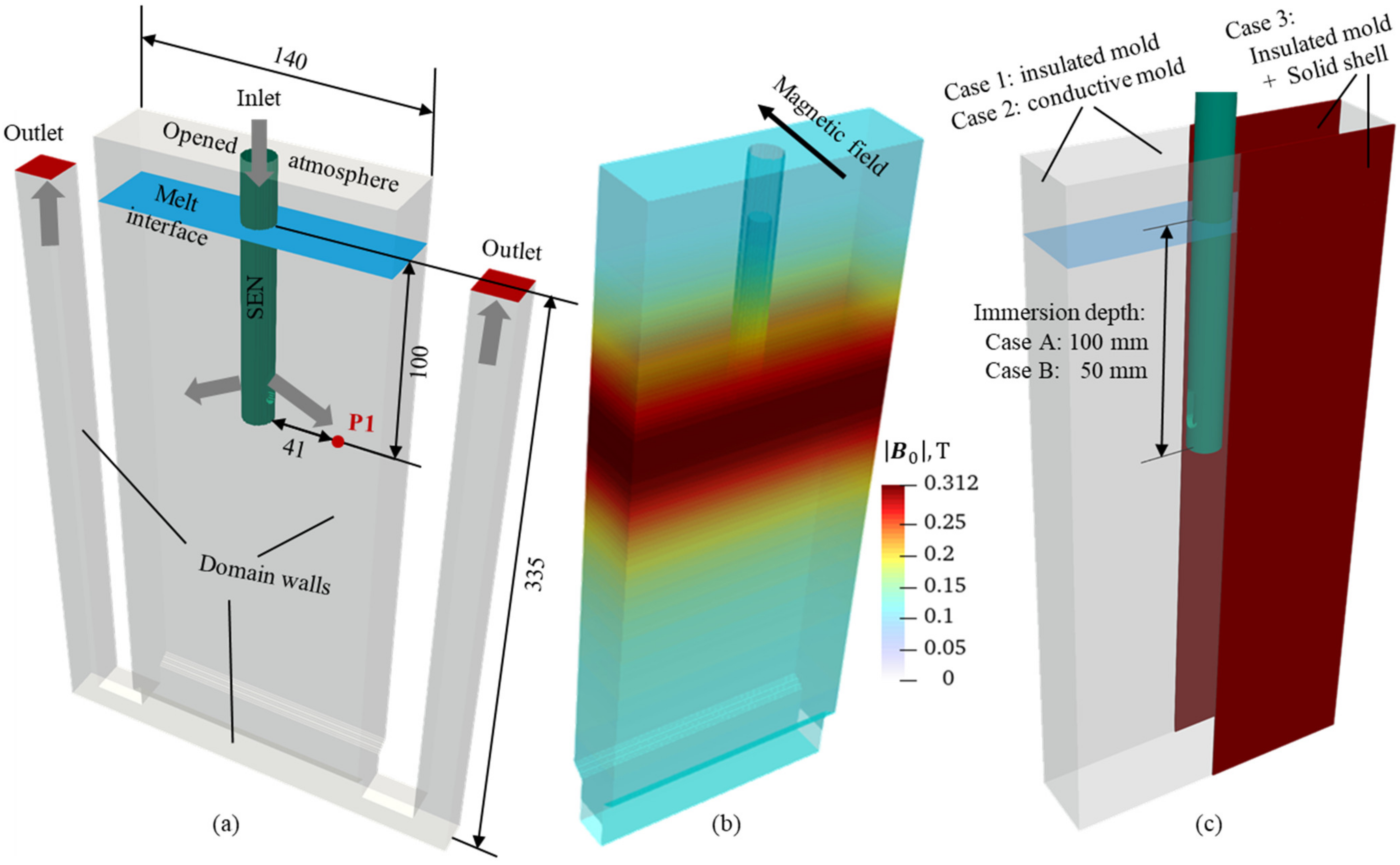
2. Materials and Methods
3. Results
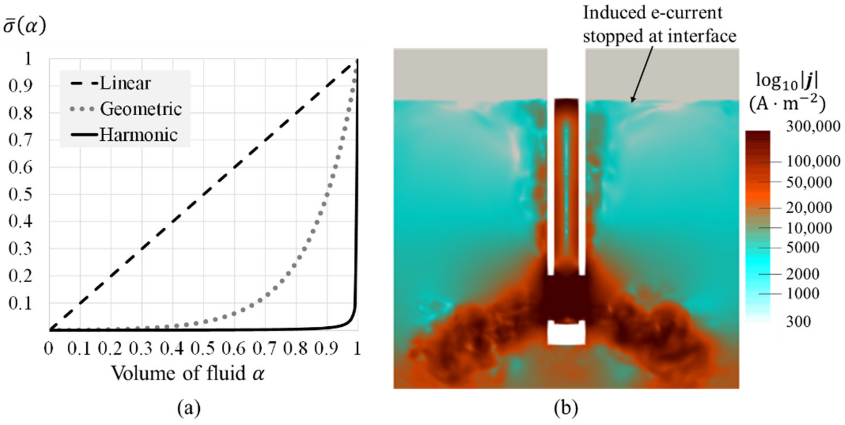
3.1. Handling Electrical Conductivity on Interface
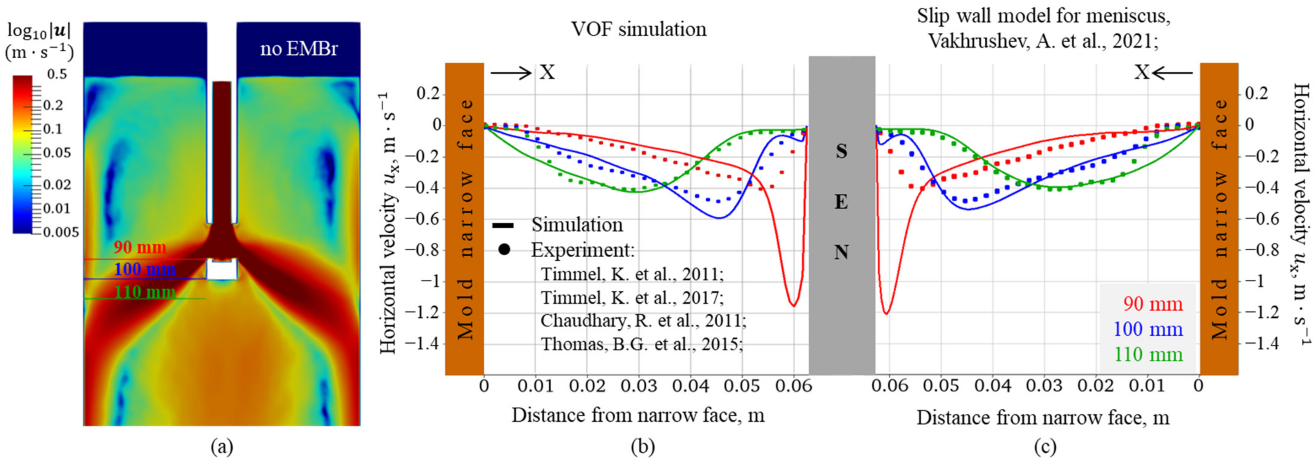
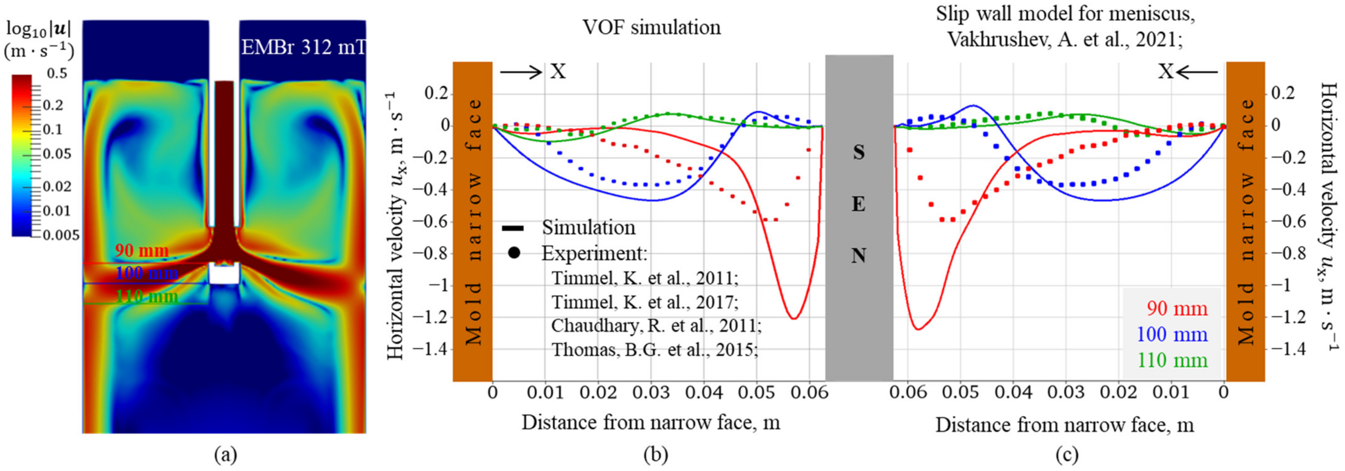
3.2. Model Verification
3.3. Case Studies
4. Discussion
4.1. MHD Turbulence
4.2. Time-Averaged Flow Field
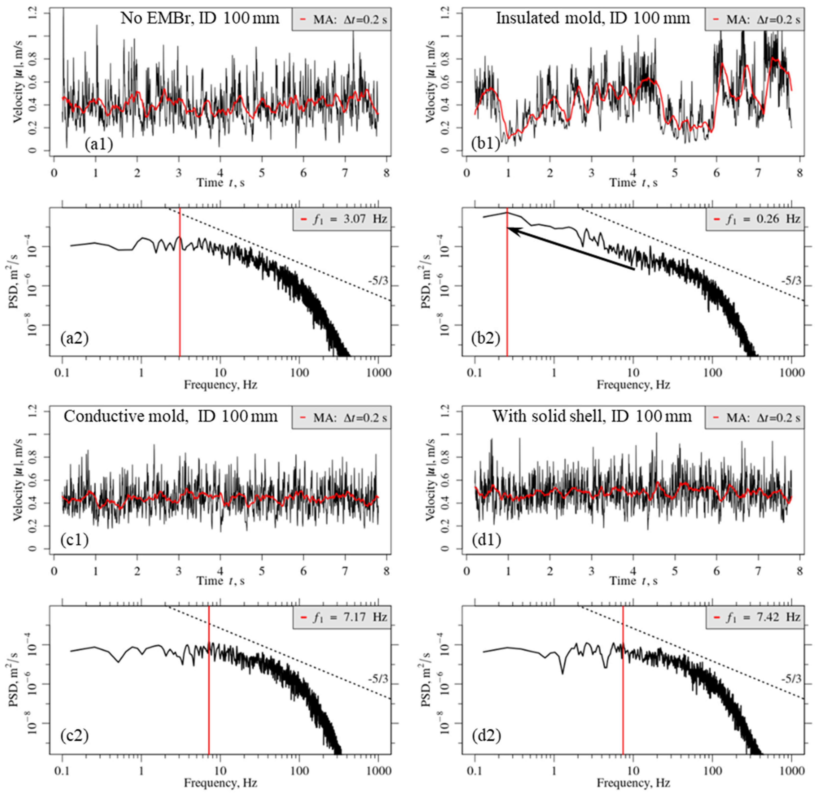
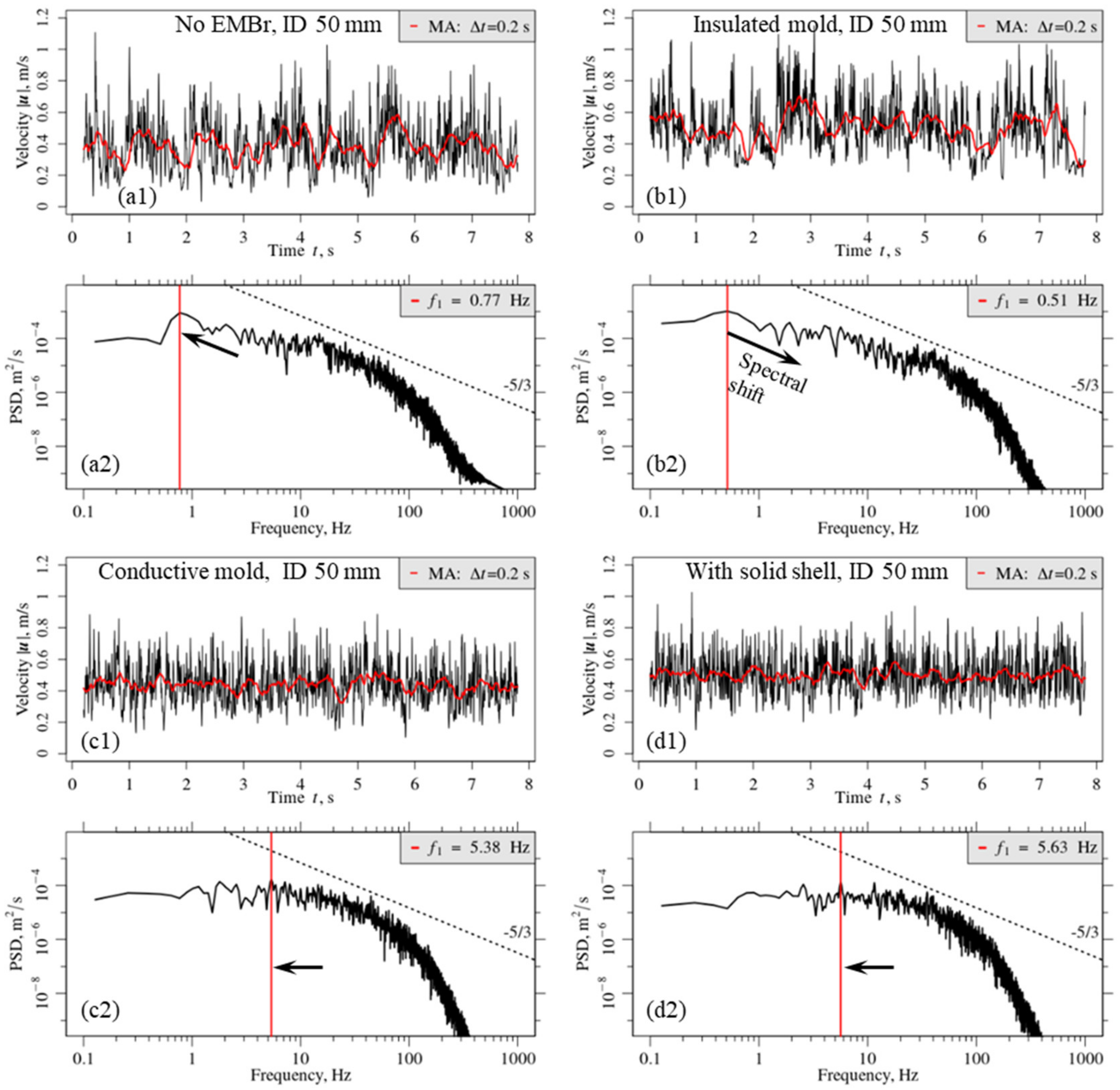
4.3. Power Spectral Density Analysis
5. Conclusions
Supplementary Materials
Author Contributions
Funding
Institutional Review Board Statement
Informed Consent Statement
Data Availability Statement
Acknowledgments
Conflicts of Interest
References
- Lee, P.D.; Ramirez-Lopez, P.E.; Mills, K.C.; Santillana, B. Review: The “Butterfly Effect” in Continuous Casting. Ironmak. Steelmak. 2012, 39, 244–253. [Google Scholar] [CrossRef]
- Mills, K.C.; Ramirez-Lopez, P.; Lee, P.D.; Santillana, B.; Thomas, B.G.; Morales, R. Looking into Continuous Casting Mould. Ironmak. Steelmak. 2014, 41, 242–249. [Google Scholar] [CrossRef]
- Lopez, P.E.R.; Jalali, P.N.; Björkvall, J.; Sjöström, U.; Nilsson, C. Recent Developments of a Numerical Model for Continuous Casting of Steel: Model Theory, Setup and Comparison to Physical Modelling with Liquid Metal. ISIJ Int. 2014, 54, 342–350. [Google Scholar] [CrossRef]
- Thomas, B.G. Review on Modeling and Simulation of Continuous Casting. Steel Res. Int. 2018, 89, 1700312. [Google Scholar] [CrossRef]
- Hibbeler, L.C.; Thomas, B.G. Mold Slag Entrainment Mechanisms in Continuous Casting Molds. Iron Steel Technol. 2013, 10, 121–136. [Google Scholar]
- Liu, Z.; Li, B.; Vakhrushev, A.; Wu, M.; Ludwig, A. Physical and Numerical Modeling of Exposed Slag Eye in Continuous Casting Mold Using Euler–Euler Approach. Steel Res. Int. 2019, 90, 1800117. [Google Scholar] [CrossRef]
- Srivastava, A.; Chattopadhyay, K. Macroscopic Mechanistic Modeling for the Prediction of Mold Slag Exposure in a Continuous Casting Mold. Met. Mater. Trans. B 2022, 53, 1018–1035. [Google Scholar] [CrossRef]
- Iguchi, M.; Yoshida, J.; Shimizu, T.; Mizuno, Y. Model Study on the Entrapment of Mold Powder into Molten Steel. ISIJ Int. 2000, 40, 685–691. [Google Scholar] [CrossRef]
- Yamashita, S.; Iguchi, M. Mechanism of Mold Powder Entrapment Caused by Large Argon Bubble in Continuous Casting Mold. ISIJ Int. 2001, 41, 1529–1531. [Google Scholar] [CrossRef]
- Yoshida, J.; Ohmi, T.; Iguchi, M. Cold Model Study of the Effects of Density Difference and Blockage Factor on Mold Powder Entrainment. ISIJ Int. 2005, 45, 1160–1164. [Google Scholar] [CrossRef]
- Kasai, N.; Iguchi, M. Water-Model Experiment on Melting Powder Trapping by Vortex in the Continuous Casting Mold. ISIJ Int. 2007, 47, 982–987. [Google Scholar] [CrossRef]
- Hagemann, R.; Schwarze, R.; Heller, H.P.; Scheller, P.R. Model Investigations on the Stability of the Steel-Slag Interface in Continuous-Casting Process. Met. Mater. Trans. B 2013, 44, 80–90. [Google Scholar] [CrossRef]
- Saeedipour, M.; Puttinger, S.; Doppelhammer, N.; Pirker, S. Investigation on Turbulence in the Vicinity of Liquid-Liquid Interfaces—Large Eddy Simulation and PIV Experiment. Chem. Eng. Sci. 2019, 198, 98–107. [Google Scholar] [CrossRef]
- Puttinger, S.; Saeedipour, M. Time-Resolved PIV Measurements of a Deflected Submerged Jet Interacting with Liquid-Gas and Liquid-Liquid Interfaces. Exp. Comput. Multiph. Flow 2022, 4, 175–189. [Google Scholar] [CrossRef]
- Bernhard, C.; Hiebler, H.; Wolf, M.M. How Fast Can We Cast? Ironmak. Steelmak. 2000, 27, 450–454. [Google Scholar] [CrossRef]
- SenGupta, A.; Santillana, B.; Sridhar, S.; Auinger, M. A Multiscale-Based Approach to Understand Dendrite Deflection in Continuously Cast Steel Slab Samples. Met. Mater. Trans. A 2021, 52, 3413–3422. [Google Scholar] [CrossRef]
- Wang, C.; Liu, Z.; Li, B. Combined Effects of EMBr and SEMS on Melt Flow and Solidification in a Thin Slab Continuous Caster. Metals 2021, 11, 948. [Google Scholar] [CrossRef]
- Vakhrushev, A.; Kharicha, A.; Karimi-Sibaki, E.; Wu, M.; Ludwig, A.; Nitzl, G.; Tang, Y.; Hackl, G.; Watzinger, J. Modeling Asymmetric Flow in the Thin-Slab Casting Mold under Electromagnetic Brake. Steel Res. Int. 2022, 93, 2200088. [Google Scholar] [CrossRef]
- Lu, H.; Zhong, Y.; Ren, W.; Ren, Z.; Lei, Z. Effect of Electromagnetic Brake on Transient Asymmetric Flow, Solidification, and Inclusion Transport in a Slab Continuous Casting. Steel Res. Int. 2022, 93, 2200518. [Google Scholar] [CrossRef]
- Timmel, K.; Eckert, S.; Gerbeth, G. Experimental Investigation of the Flow in a Continuous-Casting Mold under the Influence of a Transverse, Direct Current Magnetic Field. Met. Mater. Trans. B 2011, 42, 68–80. [Google Scholar] [CrossRef]
- Timmel, K.; Kratzsch, C.; Asad, A.; Schurmann, D.; Schwarze, R.; Eckert, S. Experimental and Numerical Modeling of Fluid Flow Processes in Continuous Casting: Results from the LIMMCAST-Project. IOP Conf. Ser. Mater. Sci. Eng. 2017, 228, 012019. [Google Scholar] [CrossRef]
- Chaudhary, R.; Ji, C.; Thomas, B.G.; Vanka, S.P. Transient Turbulent Flow in a Liquid-Metal Model of Continuous Casting, Including Comparison of Six Different Methods. Met. Mater. Trans. B 2011, 42, 987–1007. [Google Scholar] [CrossRef]
- Thomas, B.G.; Singh, R.; Vanka, S.P.; Timmel, K.; Eckert, S.; Gerbeth, G. Effect of Single-Ruler Electromagnetic Braking (EMBr) Location on Transient Flow in Continuous Casting. J. Manuf. Sci. Prod. 2015, 15, 93–104. [Google Scholar] [CrossRef]
- Liu, Z.; Vakhrushev, A.; Wu, M.; Karimi-Sibaki, E.; Kharicha, A.; Ludwig, A.; Li, B. Effect of an Electrically-Conducting Wall on Transient Magnetohydrodynamic Flow in a Continuous-Casting Mold with an Electromagnetic Brake. Metals 2018, 8, 609. [Google Scholar] [CrossRef]
- Vakhrushev, A.; Kharicha, A.; Liu, Z.; Wu, M.; Ludwig, A.; Nitzl, G.; Tang, Y.; Hackl, G.; Watzinger, J. Electric Current Distribution During Electromagnetic Braking in Continuous Casting. Met. Mater. Trans. B 2020, 51, 2811–2828. [Google Scholar] [CrossRef]
- Vakhrushev, A.; Kharicha, A.; Karimi-Sibaki, E.; Wu, M.; Ludwig, A.; Nitzl, G.; Tang, Y.; Hackl, G.; Watzinger, J.; Eckert, S. Generation of Reverse Meniscus Flow by Applying an Electromagnetic Brake. Met. Mater. Trans. B 2021, 52, 3193–3207. [Google Scholar] [CrossRef]
- Asad, A.; Kratzsch, C.; Schwarze, R. Numerical Investigation of the Free Surface in a Model Mold. Steel Res. Int. 2016, 87, 181–190. [Google Scholar] [CrossRef]
- Weller, H.G.; Tabor, G.; Jasak, H.; Fureby, C. A Tensorial Approach to Computational Continuum Mechanics Using Object-Oriented Techniques. Comput. Phys. 1998, 12, 620. [Google Scholar] [CrossRef]
- Saeedipour, M.; Vincent, S.; Pirker, S. Large Eddy Simulation of Turbulent Interfacial Flows Using Approximate Deconvolution Model. Int. J. Multiph. Flow 2019, 112, 286–299. [Google Scholar] [CrossRef]
- Roenby, J.; Bredmose, H.; Jasak, H. A Computational Method for Sharp Interface Advection. R. Soc. Open Sci. 2016, 3, 160405. [Google Scholar] [CrossRef]
- Gamet, L.; Scala, M.; Roenby, J.; Scheufler, H.; Pierson, J.-L. Validation of Volume-of-Fluid OpenFOAM® IsoAdvector Solvers Using Single Bubble Benchmarks. Comput. Fluids 2020, 213, 104722. [Google Scholar] [CrossRef]
- Esteban, A.; López, J.; Gómez, P.; Zanzi, C.; Roenby, J.; Hernández, J. A Comparative Study of Two Open-Source State-of-the-Art Geometric VOF Methods. Comput. Fluids 2023, 250, 105725. [Google Scholar] [CrossRef]
- Smolyanov, I.A.; Shmakov, E.I.; Baake, E.; Guglielmi, M. Verification of the Code to Calculate Duct Flow Affected by External Magnetic Field. Comp. Contin. Mech. 2021, 14, 322–332. [Google Scholar] [CrossRef]
- Kharicha, A.; Vakhrushev, A.; Karimi-Sibaki, E.; Wu, M.; Ludwig, A. Reverse Flows and Flattening of a Submerged Jet under the Action of a Transverse Magnetic Field. Phys. Rev. Fluids 2021, 6, 123701. [Google Scholar] [CrossRef]
- Davidson, P.A. An Introduction to Magnetohydrodynamics, 1st ed.; Cambridge University Press: Cambridge, UK, 2001; ISBN 978-0-521-79487-9. [Google Scholar]
- Ni, M.-J.; Munipalli, R.; Huang, P.; Morley, N.B.; Abdou, M.A. A Current Density Conservative Scheme for Incompressible MHD Flows at a Low Magnetic Reynolds Number. Part II: On an Arbitrary Collocated Mesh. J. Comput. Phys. 2007, 227, 205–228. [Google Scholar] [CrossRef]
- Hirt, C.W.; Nichols, B.D. Volume of Fluid (VOF) Method for the Dynamics of Free Boundaries. J. Comput. Phys. 1981, 39, 201–225. [Google Scholar] [CrossRef]
- Ubbink, O. Numerical Prediction of Two Fluid Systems with Sharp Interfaces. Ph.D. Thesis, Imperial College of Science, London, UK, 1997. [Google Scholar]
- Ubbink, O.; Issa, R.I. A Method for Capturing Sharp Fluid Interfaces on Arbitrary Meshes. J. Comput. Phys. 1999, 153, 26–50. [Google Scholar] [CrossRef]
- Vakhrushev, A.; Menghuai, W.; Ludwig, A.; Tang, Y.; Nitzl, G.; Hackl, G. Experimental Verification of the 3-Phase Continuous Casting Simulation Using a Water Model. In Proceedings of the 8th ECCC Conference, on Storage Device, Graz, Austria, 23–26 June 2014; p. 10. [Google Scholar]
- Brackbill, J.U.; Kothe, D.B.; Zemach, C. A Continuum Method for Modeling Surface Tension. J. Comput. Phys. 1992, 100, 335–354. [Google Scholar] [CrossRef]
- Boris, J.P.; Book, D.L. Flux-Corrected Transport. I. SHASTA, a Fluid Transport Algorithm That Works. J. Comput. Phys. 1973, 11, 38–69. [Google Scholar] [CrossRef]
- Zalesak, S.T. Fully Multidimensional Flux-Corrected Transport Algorithms for Fluids. J. Comput. Phys. 1979, 31, 335–362. [Google Scholar] [CrossRef]
- Vakhrushev, A.; Kharicha, A.; Liu, Z.; Wu, M.; Ludwig, A.; Nitzl, G.; Tang, Y.; Hackl, G.; Watzinger, J. Optimizing the Flow Conditions in the Thin-Slab Casting Mold Using Electromagnetic Brake. In Proceedings of the 8th International SteelSim Conference, AIST, Toronto, ON, Canada, 13–15 August 2019; pp. 615–619. [Google Scholar]
- Vakhrushev, A.; Kharicha, A.; Wu, M.; Ludwig, A.; Nitzl, G.; Tang, Y.; Hackl, G.; Watzinger, J.; Rodrigues, C.M.G. Modelling Viscoplastic Behavior of Solidifying Shell under Applied Electromagnetic Breaking during Continuous Casting. IOP Conf. Ser. Mater. Sci. Eng. 2020, 861, 012015. [Google Scholar] [CrossRef]
- Plevachuk, Y.; Sklyarchuk, V.; Eckert, S.; Gerbeth, G.; Novakovic, R. Thermophysical Properties of the Liquid Ga–In–Sn Eutectic Alloy. J. Chem. Eng. Data 2014, 59, 757–763. [Google Scholar] [CrossRef]
- Pawar, S.D.; Murugavel, P.; Lal, D.M. Effect of Relative Humidity and Sea Level Pressure on Electrical Conductivity of Air over Indian Ocean. J. Geophys. Res. 2009, 114, D02205. [Google Scholar] [CrossRef]
- Hunt, J.C.R.; Wray, A.A.; Moin, P. Eddies, Streams, and Convergence Zones in Turbulent Flows. In Proceedings of the Summer Program 1988, Center for Turbulence Research Report CTR-S88, Stanford, CA, USA, 27 June–22 July 1988; pp. 193–208. [Google Scholar]
- Kolář, V. Vortex Identification: New Requirements and Limitations. Int. J. Heat Fluid Flow 2007, 28, 638–652. [Google Scholar] [CrossRef]
- Kobayashi, H. Large Eddy Simulation of Magnetohydrodynamic Turbulent Channel Flows with Local Subgrid-Scale Model Based on Coherent Structures. Phys. Fluids 2006, 18, 045107. [Google Scholar] [CrossRef]
- Schurmann, D.; Glavinić, I.; Willers, B.; Timmel, K.; Eckert, S. Impact of the Electromagnetic Brake Position on the Flow Structure in a Slab Continuous Casting Mold: An Experimental Parameter Study. Met. Mater. Trans. B 2020, 51, 61–78. [Google Scholar] [CrossRef]
- R Core Team. R: A Language and Environment for Statistical Computing; R Foundation for Statistical Computing: Vienna, Austria, 2022. [Google Scholar]


| Case Name | Immersion Depth (mm) | EMBr Power (mT) | Domain Electrical Conductivity |
|---|---|---|---|
| Case 0A | 100 | 0 | - |
| Case 0B | 50 | 0 | - |
| Case 1A | 100 | 312 | Insulated mold |
| Case 2A | 100 | 312 | Conductive mold |
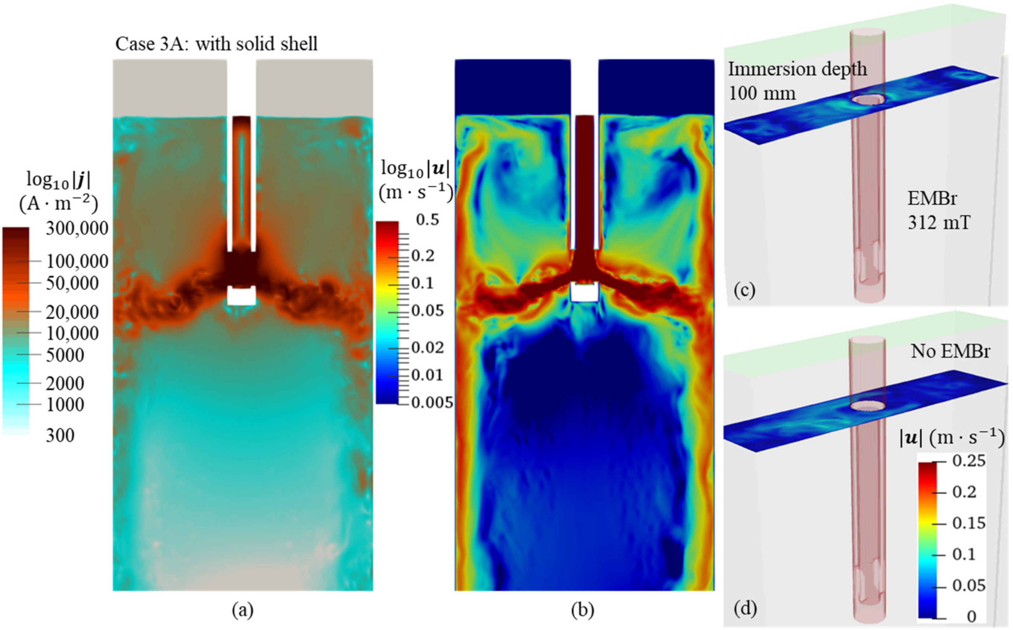
| Case 3A | 100 | 312 | Insulated mold with shell |
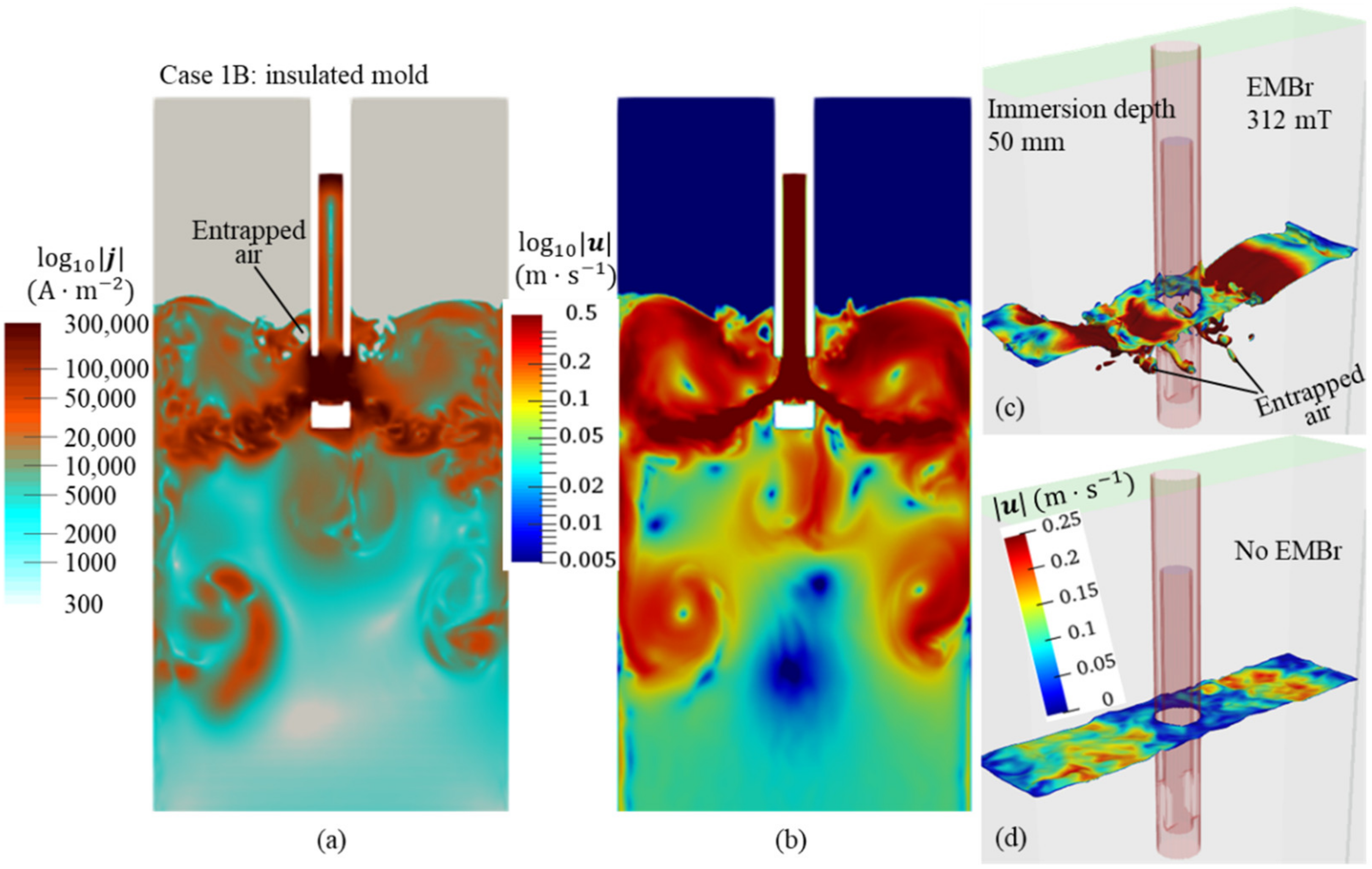
| Case 1B | 50 | 312 | Insulated mold |
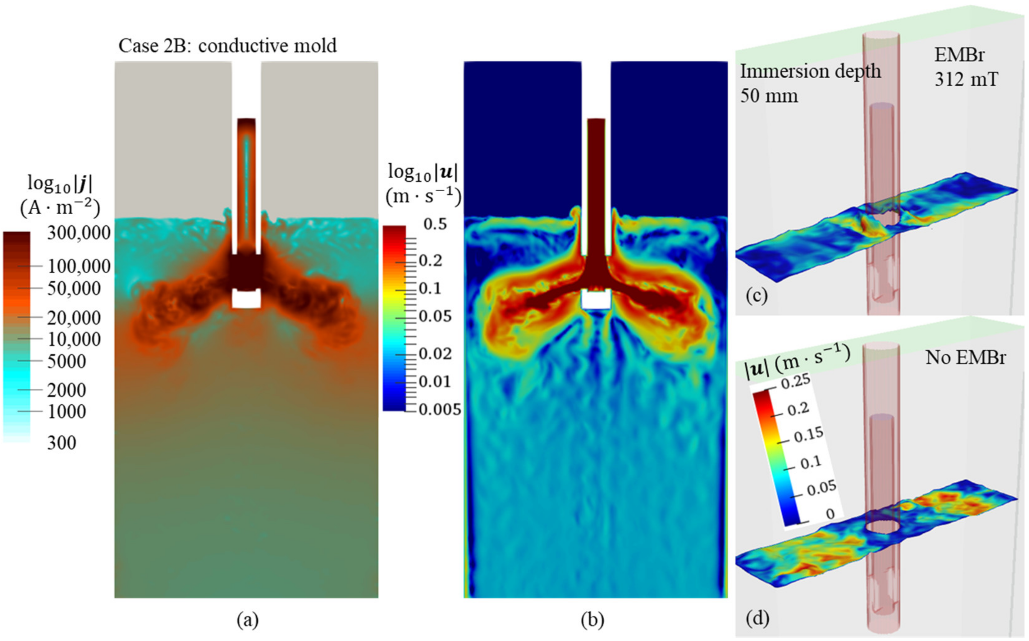
| Case 2B | 50 | 312 | Conductive mold |
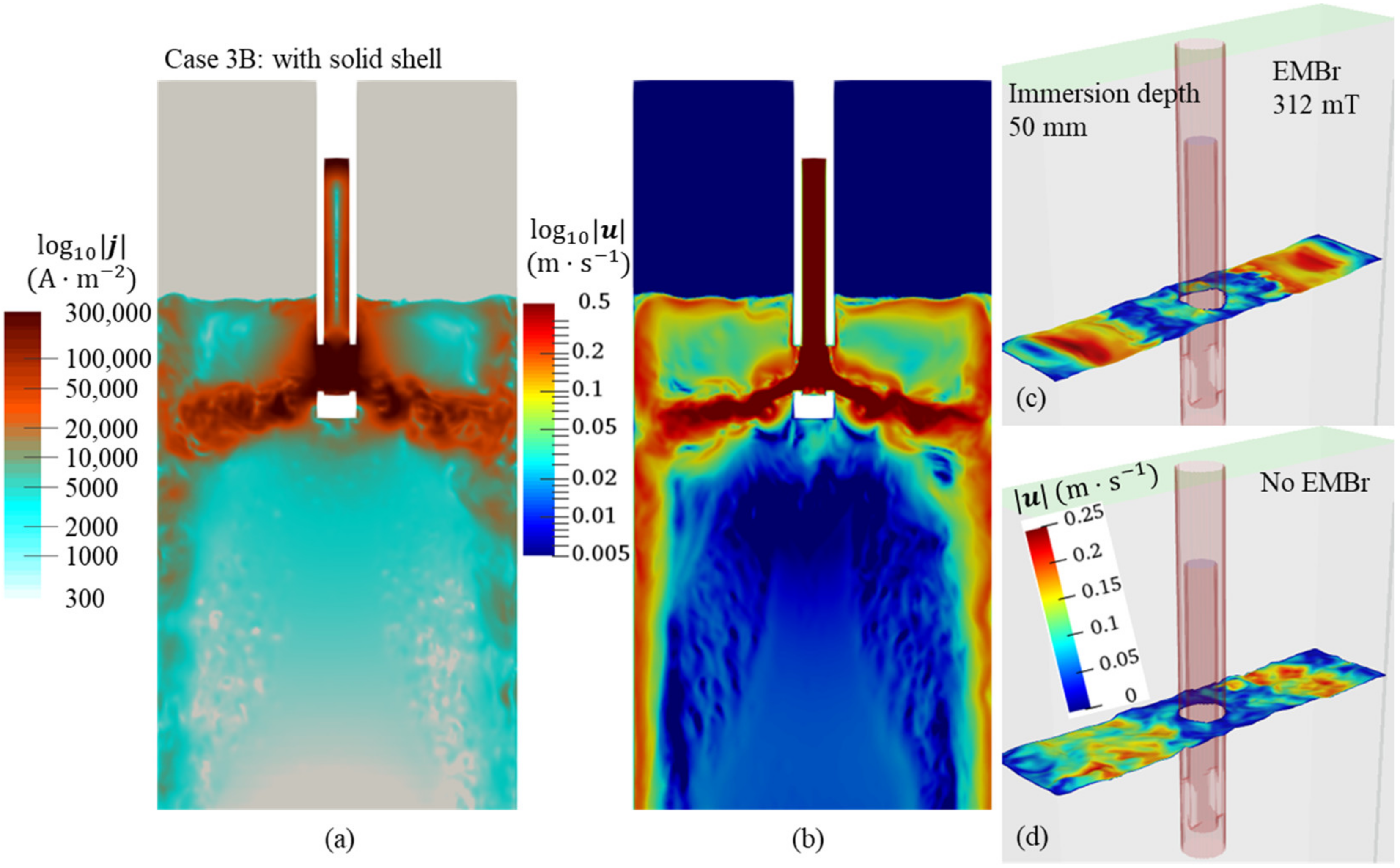
| Case 3B | 50 | 312 | Insulated mold with shell |
Disclaimer/Publisher’s Note: The statements, opinions and data contained in all publications are solely those of the individual author(s) and contributor(s) and not of MDPI and/or the editor(s). MDPI and/or the editor(s) disclaim responsibility for any injury to people or property resulting from any ideas, methods, instructions or products referred to in the content. |
© 2023 by the authors. Licensee MDPI, Basel, Switzerland. This article is an open access article distributed under the terms and conditions of the Creative Commons Attribution (CC BY) license (https://creativecommons.org/licenses/by/4.0/).
Share and Cite
Vakhrushev, A.; Karimi-Sibaki, E.; Bohacek, J.; Wu, M.; Ludwig, A.; Tang, Y.; Hackl, G.; Nitzl, G.; Watzinger, J.; Kharicha, A. Impact of Submerged Entry Nozzle (SEN) Immersion Depth on Meniscus Flow in Continuous Casting Mold under Electromagnetic Brake (EMBr). Metals 2023, 13, 444. https://doi.org/10.3390/met13030444
Vakhrushev A, Karimi-Sibaki E, Bohacek J, Wu M, Ludwig A, Tang Y, Hackl G, Nitzl G, Watzinger J, Kharicha A. Impact of Submerged Entry Nozzle (SEN) Immersion Depth on Meniscus Flow in Continuous Casting Mold under Electromagnetic Brake (EMBr). Metals. 2023; 13(3):444. https://doi.org/10.3390/met13030444
Chicago/Turabian StyleVakhrushev, Alexander, Ebrahim Karimi-Sibaki, Jan Bohacek, Menghuai Wu, Andreas Ludwig, Yong Tang, Gernot Hackl, Gerald Nitzl, Josef Watzinger, and Abdellah Kharicha. 2023. "Impact of Submerged Entry Nozzle (SEN) Immersion Depth on Meniscus Flow in Continuous Casting Mold under Electromagnetic Brake (EMBr)" Metals 13, no. 3: 444. https://doi.org/10.3390/met13030444
APA StyleVakhrushev, A., Karimi-Sibaki, E., Bohacek, J., Wu, M., Ludwig, A., Tang, Y., Hackl, G., Nitzl, G., Watzinger, J., & Kharicha, A. (2023). Impact of Submerged Entry Nozzle (SEN) Immersion Depth on Meniscus Flow in Continuous Casting Mold under Electromagnetic Brake (EMBr). Metals, 13(3), 444. https://doi.org/10.3390/met13030444