Multi-Objective Modified Differential Evolution Methods for the Optimal Parameters of Aluminum Friction Stir Welding Processes of AA6061-T6 and AA5083-H112

Abstract

This study introduces a modified differential evolution approach (MoDE) for evaluating the optimal objective and parameter values of the friction stir welding (FSW) process of dissimilar materials: AA5083 and AA6061. The aim of this study is to investigate the ultimate (UTS), maximum hardness (MH), and minimum heat input (HI) of the weld zone. The controlled welding parameters were shoulder diameter, rotation speed, welding speed, tilt angle, pin type, reinforcement particle type, and tool pin movement direction. The D-optimal experimental design method was used to create the experiment and obtain the mathematical model for optimizing the targeted objectives. The optimal rotational speed, welding speed, shoulder diameter, tilt angle, pin-type, additive type, and tool pin movement are 1162.81 rpm, 52.73 mm/min, 21.17 mm, 2.37 degrees, straight cylindrical, silicon carbide, and straight movement direction, respectively. The optimal values for UTS, MH, and HI are 264.68 MPa, 105.56 HV, and 415.26 °C, respectively. The MoDE outcome exceeded particle swarm optimization (PSO), the original differential evolution algorithm (DE), and the D-optimal design (experiment) results. The MoDE provides better UTS, MH, and HI than other approaches by an average of 8.04%, 4.44%, and 2.44%, respectively. In particular, when comparing results produced by using various approaches, we discovered that the MoDE results are 7.45%, 4.45%, and 3.50% better than PSO, DE, and the experimental results, respectively. All methods were evaluated for their reliability by comparing the results of actual experiments to those predicted by theory, and we discovered that the MoDE yielded the smallest percentage difference between the two, at 1.49%, while PSO and DE yielded differences of 5.19% and 3.71%, respectively.

1. Introduction

Aluminum alloys are prominent materials used in several industries, such as in aircraft, railway bodies, electric cars, telecommunications, electric and electronic devices, etc. Their outstanding properties include their high toughness, high corrosion resistance, high strength, light weight, and good weldability [1,2,3,4]. Various aluminum alloys are used in the construction of products with both similar [5,6] and dissimilar materials [1]. In particular, aluminum grades AA5083 and AA6061 are used in the construction of aircraft, marine vehicles, and railways [7,8], where it is necessary to join dissimilar aluminum materials. The difficulty in using dissimilar materials in fusion welding stems from their different properties, which lead to defects and changes to microstructures after welding. Therefore, the friction stir welding process (FSW) is used to create important position joints to aid in reducing problems with changed structures and eliminate flaws in weld seams [9,10], leading to superior weld quality [11,12] and decreasing the time needed to join materials when compared with other welding processes [13,14,15,16].

The use of different material welding processes influences the weld seam’s desirability, and an exceptional mechanical property obtained after welding is its high strength [17,18,19,20,21]. The many process parameters of two different types of material create several barriers for the generation of high-performance weld seams. The use of different materials makes it difficult to set the relative parameters in FSW and will affect the microstructure, making it nonhomogeneous and potentially creating micro-cracks due to the different thermal expansion processes of the material [22] and the heat generation process.

Given the information in Table 1, the most relevant factors for FSW are rotation speed and welding speed. The objective of all studies is to figure out the optimal value for these two factors. The shoulder diameters of the weld tool have been the subject of 20 out of 22 studies, but only 54.45% of researchers have been interested in determining its ideal value in FSW. In this work, the parameters of each category have been investigated. These parameters include pin type, the direction of tool movement, and reinforcement particle type. Five researchers were interested in utilizing a straight cylindrical as the pin tool [2,15,23,24,25], four researchers used a threaded cylindrical tool [2,18,26,27], and only two researchers disclosed the effect of using a hexagonal cylindrical tool [23,24]. To the best of our knowledge, there is no research that compares the use of all three types of tool pins. Consequently, this is the first research gap identified in Table 1.

Silicon carbide [18,19,20,27,28,29] and aluminum oxide [26] are among the previously studied reinforcing particle types (RPTs). In addition, there is no research comparing the effectiveness of these two RPT. We will be the first researchers to compare the relative effectiveness of these two RPTs in this study. Lastly, we discovered from past research that the straight movement of the tool has been researched; however, no additional tool movements have been studied, at least not for joining the target material. The efficiency of these two types of tool movement, zigzag and circular movement, as described by [30,31], has not yet been studied. This is the first study in the field of FSW to evaluate and compare the effectiveness of different forms of tool movement. At this point, the gap in research that we found is related with the parameters and the target response of the FSW used to join AA5083 and AA6061, and they are outlined as follows:

(1)

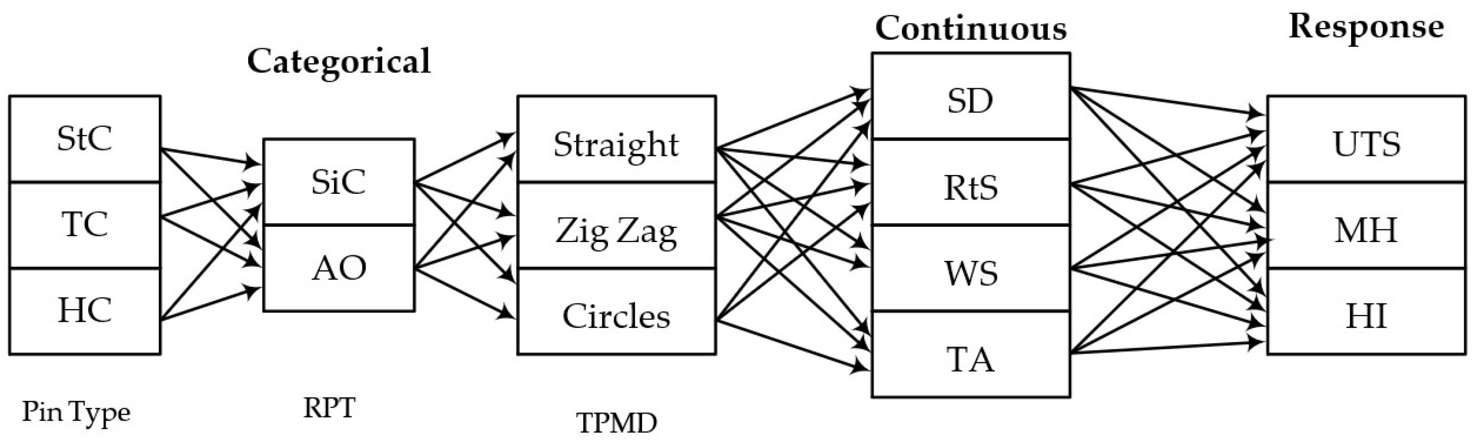
No research exists that can propose the optimal values for all factors and responses involved. (1) Shoulder diameter (SD), rotation speed (RtS), welding peed (WS), tilt angle (TA), tool pin movement direction (TPMD), reinforcement particles type (RPT), and pin type are the relevant parameters (PT). (2) Ultimate tensile strength (UTS), maximum hardness (MH), and heat input are the desired responses (HI).

(2)

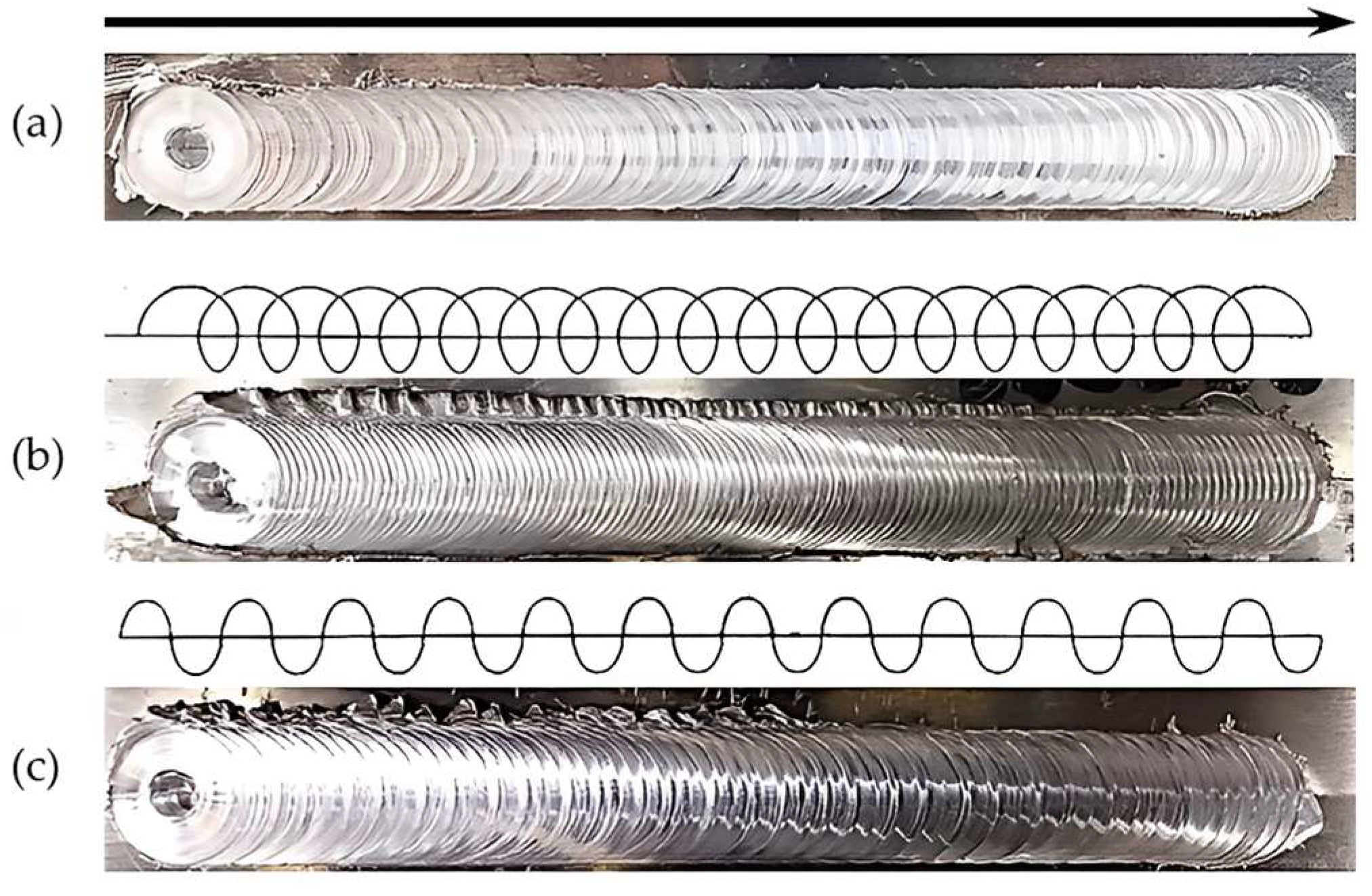
No research has uncovered the distinction between different tool pin movement directions (TPMDs). Movements such as straight, zigzag, and circle are among the TPMDs suggested by the relevant literature.

(3)

No research has compared the use of silicon carbide and aluminum oxide as the FSW’s additive.

The information in

Table 2. Finding an optimal method for friction stir welding processes.

Material	Methods												Response			% Error
	Statistical Method							Heuristic					Exp.	Predict	Confirm
	RSM	Taguchi	GRA	ANOVA	Shannon	Pareto Front.	TOPSIS	ANN	GA	ANFIS	SA	MoDE
AA6082-T6 [33]	-	✓	✓	-	-	-	-	✓		-	-	-	221.8	212.41	-	4.42
AA2219 [34]	-	✓	-	-	-	-	-	✓	✓	-	-	-	-	330.98	341.27	3.11
AA6063-T6 [38]	✓	-	-	✓	-	-	-	-	-	-	-	-	-	146.83	147.51	0.46
AA5086-H32 [39]	✓	-	-	✓	-	-	-	-	-	-	-	-	-	193.33	190.33	1.55
AA7075 [40]	✓	-	-	-	-	-	-	-	-	✓	✓	-	-	221.9	227	2.30
AA6061-T6 [41]	✓	-	-	-	-	-	-	-	-	-	-	✓	-	294.84	295	0.05
AA6101/Pure Copper [32]	-	✓	✓	-	-	-	✓	-	-	-	-	-	-	202.57	206.56	1.97
AA6061-T6/AA7075-T6 [35]	✓	-	-	-	✓	✓	✓	-	-	-	-	-	-	245.95	252.23	2.55
AA5083/AA6063 [36]	-	✓	✓	-	-	-	-	-	-	-	-	-	-	136.2	168	23.35
AA5052-H32/AA5754-H22 [37]	-	✓	✓	-	-	-	-	-	-	-	-	-	180.52	-	175	3.15

Note: RSM; Response Surface Methodology, GRA; grey relational analysis, ANN; Artificial neural network, GA; Genetic Algorithm, SA; Simulated Annealing. ANFIS; Adaptive Neuro-Fuzzy Inference System, MoDE; Modified Differential Evolution. Exp; Experiment.

is utilized to reveal the approach used to determine the optimal parameters and responses of the FSW. The methodologies utilized in the relevant literature can be split into two distinct categories. The first category involves statistical approaches, such as RSM, Taguchi, and ANOVA, which have been utilized most frequently to determine the best parameters [32,33,34,35,36,37,38,39,40,41]. The second group that has lately been utilized to optimize the responsiveness and value of parameters is known as heuristic techniques. These techniques include genetic algorithms (GA), simulated annealing (SA), artificial neural networks (ANN), and adaptive neuro-fuzzy inference systems (ANFIS) [27,33,34,40,41]. The effective use of heuristics has been utilized to determine the ideal welding response value. In conjunction with heuristic approaches, the pareto front analysis and technique for order of preference by similarity to ideal solution (TOPSIS) were applied to the multi-objective optimization model. The recent use of the differential evolution algorithm (DE) to solve multi-objective models [31] has been fruitful. The author updated a portion of the original procedure in order to achieve the modified version of DE [42,43] and proposed modifying the recombination process of the DE in order to acquire the neighborhood solution of the current best solution. We discovered that the modified mutation process of the original DE also plays a significant role in enhancing the current solution since it can improve the DE’s local search behavior [44]. In order to increase the solution quality of DE in the mutation process, we will build a new formula as part of this research study.

Table 1. The literature review of the parameters of friction stir welding processes.

Author	Materials	Approaches for Optimization	Continuous				Category								Response
			SD	RtS	WS	TA	Pin Type			RPT		TPMD			UTS (MPa)	McH (HV)	HI (°C)
							StC	T	H	SiC	AO	S	Z	C
Suppachai et al. (2021) [24]	SSM-ADC 12	VaNSAS	-	✓	✓	✓	✓	-	✓	-	-	✓	-	-	✓	-	-
Suppachai et al. (2021) [23]	SSM-ADC 12	MOVaNSAS	-	✓	✓	✓	✓	-	✓	-	-	✓	-	-	✓	-	-
Chennaiah et al. (2021) [13]	AA5083	-	✓	✓	✓	-	-	-	-	-	-	✓	-	-	✓	✓	-
W.F. Xu et al. (2021) [14]	AA7085-T7452	-	✓	✓	✓	✓	-	-	-	-	-	✓	-	-	✓	-	-
M. Kianezhad et al. (2019) [26]	AA5083	-	✓	✓	✓	✓	-	✓	-	-	✓	✓	-	-	✓	✓	-
Khan et al. (2018) [45]	AA5083	-	✓	✓	✓	✓	-	-	-	-	-	✓	-	-	✓	✓	-
K. Aruna Prabha et al. (2018) [46]	AA5083	-	✓	✓	✓	-	-	-	-	-	-	✓	-	-	✓	✓	-
Kumar et al. (2018) [47]	AA5083	-	✓	✓	✓	-	-	-	-	-	-	✓	-	-	✓	✓	-
Jia et al. (2022) [15]	AA5083, AA6061	-	✓	✓	✓	✓	✓	-	-	-	-	✓	-	-	✓	✓	-
Kumar et al. (2021) [4]	AA5083, AA6061	-	✓	✓	✓	✓	-	-	-	-	-	✓	-	-	✓	✓	-
Kumar et al. (2022) [7]	AA5083, AA6061	-	✓	✓	✓	✓	-	-	-	-	-	✓	-	-	✓	✓	-
Fuse et al. (2021) [25]	AA5083, AA6061	-	✓	✓	✓	-	✓	-	-	-	-	✓	-	-	-	✓	-
Kumar et al. (2020) [21]	AA5083, AA6082	DOE, ANOVA	✓	✓	✓	✓	-	-	-	-	-	✓	-	-	✓	-	-
Ramesh et al. (2020) [2]	AA5083, AA6061	Taguchi, ANOVA	✓	✓	✓	-	✓	✓	-	-	-	✓	-	-	✓	✓	-
Tayebi et al. (2019) [48]	AA5083, AA6061	-	✓	✓	✓	✓	-	-	-	-	-	✓	-	-	✓	✓	-
Bodaghi et al. (2017) [27]	AA5052	-	✓	✓	✓	-	-	✓	-	✓	-	✓	-	-	✓	✓	-
Karthikeyan et al. (2015) [28]	Al6351	Taguchi	✓	✓	✓	-	-	-	-	✓	-	✓	-	-	✓	✓	-
Rani et al. (2022) [18]	AA5083, AA6061	-	✓	✓	✓	✓	-	✓	-	✓	-	✓	-	-	✓	✓	-
Moradi et al. (2019) [20]	AA2024, AA6061	-	✓	✓	✓	✓	-	-	-	✓	-	✓	-	-	✓	-	-
Moradi et al. (2017) [29]	AA6061, AA2024	-	✓	✓	✓	✓	-	-	-	✓	-	✓	-	-	✓	✓	-
M. Tabasi et al. (2016) [19]	AA7075, AZ31	-	✓	✓	✓	-	-	-	-	✓	-	✓	-	-	✓	-	-
This work	AA5083-AA6061	D-optimal, DE, MoDE, Pareto front, TOPSIS	✓	✓	✓	✓	✓	✓	✓	✓	✓	✓	✓	✓	✓	✓	✓

Note: Continuous: SD; Shoulder Diameter, RtS; Rotation Speed, WS; Welding Speed, TA; Tilt Angle. Category: StC; Straight Cylindrical, T; Threaded Cylindrical, H; Hexagonal Cylindrical, RPT; reinforcement particles type, SiC; Silicon Carbide, AO; Aluminum Oxide. TPMD; Tool Pin Movement Direction, S; Straight, Z; Zig Zag, C; Circles. Response: UTS; Ultimate Tensile Strength, McH; Micro-Hardness, HI; Heat Input.

Table 1. The literature review of the parameters of friction stir welding processes.

Author	Materials	Approaches for Optimization	Continuous				Category								Response
			SD	RtS	WS	TA	Pin Type			RPT		TPMD			UTS (MPa)	McH (HV)	HI (°C)
							StC	T	H	SiC	AO	S	Z	C
Suppachai et al. (2021) [24]	SSM-ADC 12	VaNSAS	-	✓	✓	✓	✓	-	✓	-	-	✓	-	-	✓	-	-
Suppachai et al. (2021) [23]	SSM-ADC 12	MOVaNSAS	-	✓	✓	✓	✓	-	✓	-	-	✓	-	-	✓	-	-
Chennaiah et al. (2021) [13]	AA5083	-	✓	✓	✓	-	-	-	-	-	-	✓	-	-	✓	✓	-
W.F. Xu et al. (2021) [14]	AA7085-T7452	-	✓	✓	✓	✓	-	-	-	-	-	✓	-	-	✓	-	-
M. Kianezhad et al. (2019) [26]	AA5083	-	✓	✓	✓	✓	-	✓	-	-	✓	✓	-	-	✓	✓	-
Khan et al. (2018) [45]	AA5083	-	✓	✓	✓	✓	-	-	-	-	-	✓	-	-	✓	✓	-
K. Aruna Prabha et al. (2018) [46]	AA5083	-	✓	✓	✓	-	-	-	-	-	-	✓	-	-	✓	✓	-
Kumar et al. (2018) [47]	AA5083	-	✓	✓	✓	-	-	-	-	-	-	✓	-	-	✓	✓	-
Jia et al. (2022) [15]	AA5083, AA6061	-	✓	✓	✓	✓	✓	-	-	-	-	✓	-	-	✓	✓	-
Kumar et al. (2021) [4]	AA5083, AA6061	-	✓	✓	✓	✓	-	-	-	-	-	✓	-	-	✓	✓	-
Kumar et al. (2022) [7]	AA5083, AA6061	-	✓	✓	✓	✓	-	-	-	-	-	✓	-	-	✓	✓	-
Fuse et al. (2021) [25]	AA5083, AA6061	-	✓	✓	✓	-	✓	-	-	-	-	✓	-	-	-	✓	-
Kumar et al. (2020) [21]	AA5083, AA6082	DOE, ANOVA	✓	✓	✓	✓	-	-	-	-	-	✓	-	-	✓	-	-
Ramesh et al. (2020) [2]	AA5083, AA6061	Taguchi, ANOVA	✓	✓	✓	-	✓	✓	-	-	-	✓	-	-	✓	✓	-
Tayebi et al. (2019) [48]	AA5083, AA6061	-	✓	✓	✓	✓	-	-	-	-	-	✓	-	-	✓	✓	-
Bodaghi et al. (2017) [27]	AA5052	-	✓	✓	✓	-	-	✓	-	✓	-	✓	-	-	✓	✓	-
Karthikeyan et al. (2015) [28]	Al6351	Taguchi	✓	✓	✓	-	-	-	-	✓	-	✓	-	-	✓	✓	-
Rani et al. (2022) [18]	AA5083, AA6061	-	✓	✓	✓	✓	-	✓	-	✓	-	✓	-	-	✓	✓	-
Moradi et al. (2019) [20]	AA2024, AA6061	-	✓	✓	✓	✓	-	-	-	✓	-	✓	-	-	✓	-	-
Moradi et al. (2017) [29]	AA6061, AA2024	-	✓	✓	✓	✓	-	-	-	✓	-	✓	-	-	✓	✓	-
M. Tabasi et al. (2016) [19]	AA7075, AZ31	-	✓	✓	✓	-	-	-	-	✓	-	✓	-	-	✓	-	-
This work	AA5083-AA6061	D-optimal, DE, MoDE, Pareto front, TOPSIS	✓	✓	✓	✓	✓	✓	✓	✓	✓	✓	✓	✓	✓	✓	✓

Note: Continuous: SD; Shoulder Diameter, RtS; Rotation Speed, WS; Welding Speed, TA; Tilt Angle. Category: StC; Straight Cylindrical, T; Threaded Cylindrical, H; Hexagonal Cylindrical, RPT; reinforcement particles type, SiC; Silicon Carbide, AO; Aluminum Oxide. TPMD; Tool Pin Movement Direction, S; Straight, Z; Zig Zag, C; Circles. Response: UTS; Ultimate Tensile Strength, McH; Micro-Hardness, HI; Heat Input.

This research makes the following contributions based on what we have learned by reviewing prior related material:

(1)

We describe the methods for identifying the optimal FSW responses and parameter set based on a model with multiple objectives (seven parameters and three responses).

(2)

The heat input (HI) is introduced for the first time into a multi-objective model to reveal the optimal response of friction stir welding in collaboration with UTS and MH.

(3)

This research presents, for the first time, a comparison of the effectiveness of using several types of pin tool movement directions when welding AA6061-T6 and AA5083-H112.

(4)

The efficacy comparison of several additive chemicals (SiC and AO) for connecting AA6061-T6 and AA5083-H112 has been provided for the first time.

(5)

Initially, the modified version of the differential evolution algorithm (MoDE) was presented to determine the optimal value of the asymmetric FSW.

The remainder of this article is structured as follows. In Section 2, the related literature will be revealed, while the research material and methodology will be provided in Section 3. The experimental framework and results will be provided in Section 4. Section 5, Section 6 and Section 7 contain, respectively, the microstructure analysis, discussion, and conclusion.

2. Related Literature

The use of different material welding processes influences the weld seam’s desirability, and an exceptional mechanical property given after welding is its high strength. The many process parameters of two different types of material create several barriers for the generation of high-performance weld seams. The use of different materials makes it difficult to set the relative parameters in FSW and will affect the microstructure, making it nonhomogeneous and potentially creating micro-cracks due to the different thermal expansion processes of the material [22] and the heat generation process. The important parameters of dissimilar materials in the FSW process consist of the rotation speed, welding speed, shoulder diameter, tilt angle, and pin profile, which are affected by heat generation, plastic deformation, and material flow in welding [49]. The multitude of welding parameters make the suitable generation of relative parameters difficult. Several studies mention the qualities of weld seams produced using dissimilar material welding. The strength of the weld seam can lead to worse mechanical properties than those of the base material [50]. Previously, the heat treatment process has been used for the microstructural improvement of weld seams after the friction stir welding process [51,52], but it takes a long time and comes at a high cost [53,54,55,56]. Therefore, particle reinforcement is determined by the quality improvement of the weld seam [55,56,57,58]. Various reinforcement particles are applied in weld seam reinforcement and help increase the weld line’s strength. The type of particles used include carbon nanotube, boron carbide, aluminum oxide, and silicon carbide [45,55,56,58,59,60,61]. Aluminum oxide and silicon carbide are high-strength particles that produce low defects, a low hinderance of the material’s flow, and a good adhesion interface in the weld seam’s structure. Improving the weld seam’s quality and mechanical properties such as tensile strength and hardness depends on the type of reinforcement particles used [62,63,64,65]. Thus, aluminum oxide and silicon carbide are often chosen for reinforcement in order to increase the weld seam’s quality. However, the problem of particle reinforcement is the uneven dispersion in their structure. Formerly, in [50,66], the authors mentioned that the choice of the multi-welded tool pin’s movement direction could influence the distribution of reinforcement particles; however, it may lead to problems such as high welding process heat and broad microstructure changes, as well as causing reduced strength in the heat-affected zone. The study of the tool pin’s movement direction suited toward welding parameters can reduce problems resulting from the agglomeration of reinforcement particles and overheating in FSW [67,68,69,70,71,72]. Furthermore, welding parameter control is important, as setting them can lead to sufficient welding process heat, ultimate tensile strength, maximum hardness, and high-quality weld seam generation [45,70,72,73,74].

From the literature review, it was found that there is a lack of studies on the FSW of aluminum materials relating to tool pin movement directions and welding process heat control using a parameter method to optimize the completeness and performance of the weld seam, as shown in Table 1. This table shows the previous studies on FSW parameters and research effects. In addition, finding the optimal welding parameter can help achieve two major objectives. Previously, welding parameter control in FSW relied on designing welding parameters that can attain improvements in the performance of the weld seam. Examples include Taguchi with GRA and TOPSIS [32]; Taguchi with GRA and ANN [33]; Taguchi with ANN and GA [34]; RSM with Pareto frontier, TOPSIS, and Shannon [35]; Taguchi with GRA [36,37]; RSM with ANOVA [38,39]; and RSM with ANFIS and SA [40]. These methods show optimal condition welding and can increase the mechanical quality of weld seams, but response predictions produce high levels of error in the range from 2.24 to 15.72% [23]. Moreover, relative welding parameter generation and multi-objective response analyses can change several welding parameters at a time, reducing the accuracy of the result. In [41], the response surface method and the modified differential evolution algorithm (RSM-MDE) are used for finding the optimal welding parameter on multi-objective responses, showing a high performance in optimal solution finding, and producing a high solution accuracy of 99.95% when compared with other approaches, as shown in Table 2. The several methods taken together are used for optimizing the welding parameter, displaying their influence on increasing solution-finding accuracies. Therefore, solution finding based on the hybrid method cannot be ignored.

This research focuses on dissimilar aluminum welding with particle reinforcement in the weld seams of AA6061-T6 and AA5083-H112. The three hybrid methods used are MoDE, Pareto front, and TOPIS, which can be applied to optimal welding parameter finding and multi-objective responses analyses. The three responses consist of ultimate tensile strength (UTS), maximum hardness (MH), and minimum heat input (HI) in the welding process of FSW. In the study, the parameter types are separated into two groups: (1) continuous variables and (2) categorical variables. The four continuous variables consist of shoulder diameter, tilt angle, rotation speed, and welding speed. The three categorical variables consist of pin type, reinforcement particles type, and tool pin movement direction. Including the resulting welded seam, the microstructure will be analyzed using an optical microscope (OM), a scanning electron microscope (SEM), and an energy dispersive X-ray spectrometer (EDX).

Several studies have been conducted on friction stir welding in recent years (FSW). The use of a donor material to aid in heating workpieces without wearing down the tool or introducing more heat than necessary to the system was investigated in [44]. A novel study was conducted on the connection of overlapped nickel-based alloy 625 and marine-grade GL E36 steel plates using friction stir lap welding (FSLW). The interface microstructure and its impact on the joint’s strength are examined [75]. The authors of [76] gave a comprehensive analysis of the developments in the solid-state welding process of steels by diffusion bonding (DB) and friction stir welding (FSW). Considerable consideration was devoted to DB steel, which overcomes the challenges of segregation, cracking, and deformation stresses that are often produced by liquid-phase welding processes. Friction and wear properties and mechanisms at various temperatures of the friction stir lap welding joint process of SiCp/ZL101 and ZL101 were investigated in [77]. The study [78] examined the influence of friction stir welding settings on the weldability of aluminum alloys with similar and different metals.

Five bobbin tools with varying shoulder fillet radii were used for the bobbin tool friction stir welding (BT-FSW) of A1050-O sheets, as described in [79]. To improve the accuracy of the numerical simulation of the friction stir welding (FSW) process, the tool’s tilt angle must be considered as a crucial parameter. A previous study [80] offered a microstructural analysis of the mechanical response of several sequences of heat treatment, FSW, and CR in an Al-Mg AA5754 alloy that had not been age hardened. The thermomechanical behavior of nanoscale Al₂O₃ particles used to reinforce aluminum was investigated in [57]. The material was developed using spark plasma sintering and friction stir welding. By COMSOL MultiPhysics, the thermal stresses influencing the composite’s behavior during welding were modelled, and the results were validated by applying mechanical property assessments on the composites. Due of the higher heat input and more efficient recrystallization, the weld nugget zone becomes harder as the tool speed increases, according to research [81]. The weld generated with the fastest tool rotating speed provided a weld with the hardest weld nugget zone.

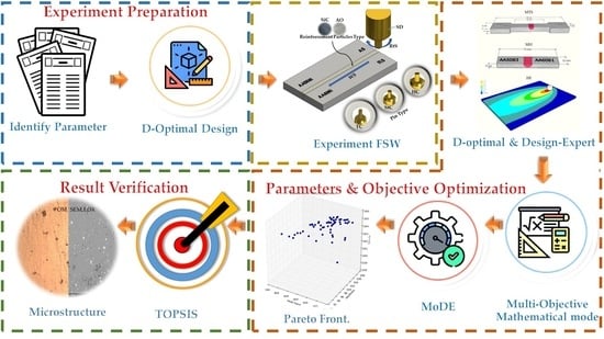
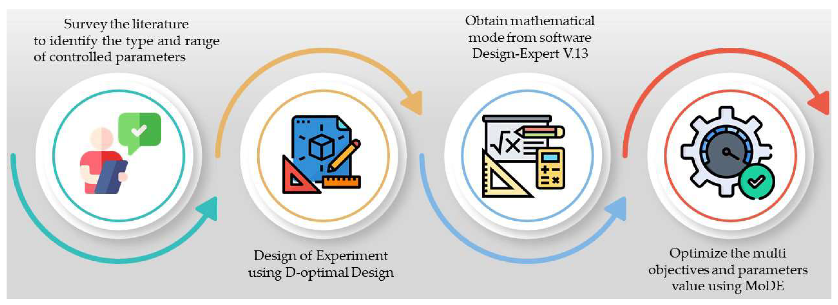
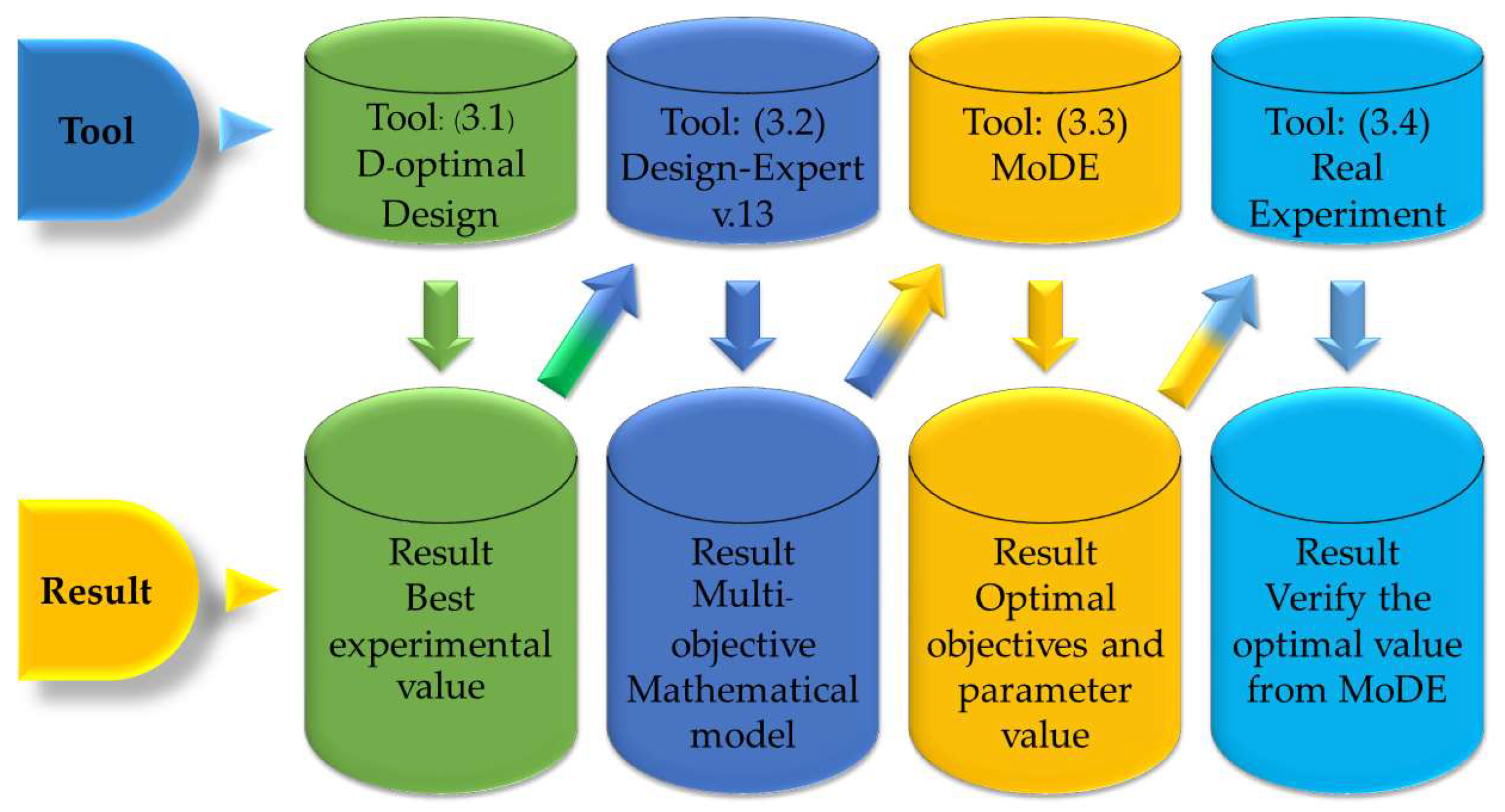
3. Materials and Methods

AA5083 and AA6061 plates measuring 200 mm in length, 75 mm in width, and 6 mm in thickness were employed for the friction stir welding research investigation.

Table 3. Chemical compositions of the base alloys.

Materials	Element (wt.%)
	Al	Ni	Ti	Ag	Zr	Sn	Pb	Co	La	B	Be
AA5083-H112	94.8	0.0021	0.0182	0.0001	0.0007	0.001	0.009	0.001	0.0005	0.004	0.001
AA6061-T6	96.6	0.0218	0.0374	0.0001	0.0094	0.0558	0.0822	0.0326	0.0115	0.0128	0.0005

and

Table 4. Mechanical properties of the base alloys.

Materials	Ultimate Tensile Strength (UTS) (MPa)	Maximum Hardness (MH) (HV)
A5083-H112	277.70	91
AA6061-T6	264.72	107

detail the chemical composition and mechanical properties ofAA5083 and AA6061. The tool material used was H13 and involved air-hardening processes. The CNC milling machine (type HAAS) was employed to FSW join the material. The research process was as follows: (1) conducting a survey to determine the number of parameters and levels of FSW, (2) constructing an experimental design using D-optimal to obtain a mathematical model, (3) performing the experiment as designed, (4) optimizing the responses for the parameters using the MoDE algorithm, and (5) verifying the results obtained in step 3. The details of the proposed procedure are as follows.

3.1. Survey Determining the Number of FSW’s Parameters and Levels

The literature review revealed that the experimental parameter types were divided into two categories: (1) continuous variables and (2) categorical variables. In this investigation, four continuous variables consisting of the shoulder diameter (SD), tilt angle (TA), rotation speed (RtS), and welding speed (WS) were utilized, as shown in Figure 1. Three categorical variables consisting of the pin type (PT), reinforcement particle type (RPT), and tool pin movement direction (TPMD) were examined, as shown in Figure 2, and the suitable heat input investigation found that the optimal heat input for the friction stir welding of AA6061 and AA5083 was within the range of 315–485 °C [52,82,83,84], which is good for welding and achieving a high weld seam quality.

Table 5. Continuous and categorical variables of the parameters in the experiment.

Continuous Variable
Parameter	Levels
	−1	1
Rotation Speed (rpm), RtS	150	1500
Welding Speed (mm/min), WS	15	135
Shoulder Diameter (mm), SD	18	25
Tilt Angle (degrees), TA	0	3
Categorical Variable
Parameter	Levels
Pin Type	Straight Cylindrical	Hexagonal Cylindrical	Threaded Cylindrical
Reinforcement Particles Type	Silicon Carbide	Aluminum Oxide	-
Tool Pin Movement Direction	Straight	Zig Zag	Circles

contains information on the parameter types.

Straight, circle, and zigzag movements are the three types of tool pin movement directions that can be observed in Figure 2. During the experiment, the effects of these three types of movement were discovered.

3.2. Designing an Experiment Using the D-Optimal Method

The D-optimal method was used to derive the experimental design from each interesting parameter using a 58-point model, with 48 minimum model points for the results, 5 points for replicates, and 5 points for the estimation of the lack of fit. The parameters were set to the upper and lower limits of −1 and 1 in the Design-Expert v. 13 software. The values of the intermediate code were calculated using Equation (1):

$$Original=\frac{Scaled\left[\left(X_{Max}+X_{min}\right)\right]+X_{Max}+X_{min}}{2}$$

(1)

where scaled denotes the value that was coded for variable X, X is the value of the variable between $X_{min}$ and $X_{Max}$, and $X_{min}$ and $X_{Max}$ are the minimum and maximum values for the specified parameter, respectively. The Design-Expert software, which incorporates the D-optimal, has been used for generations and for the experimental design and analysis.

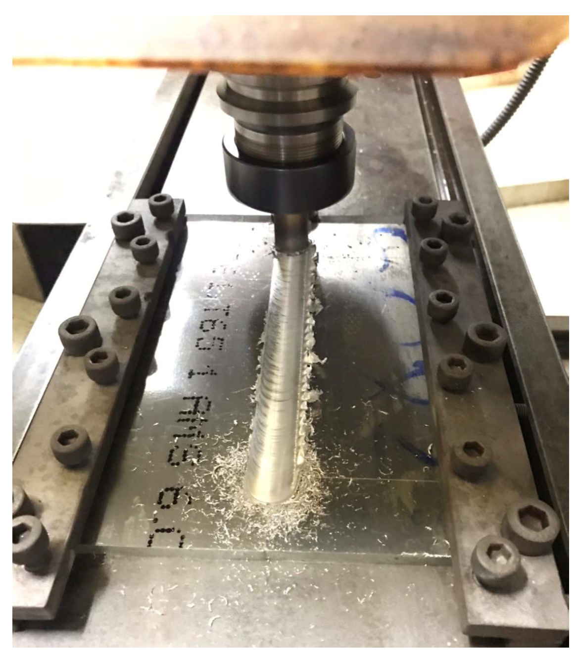
3.3. Performing the Experiment According to the Experimental Design Obtained from Section 3.2

We used a CNC milling machine to execute friction stir welding on a total of 58 parts according to the designed experiment. The combinations of the parameters for the experiment are detailed in Figure 3.

After welding, specimens were cut with a waterjet from the work pieces for testing mechanical properties (Figure 4a,b). Tensile strength, micro-hardness, and heat input were measured (Figure 4c). The tensile specimens were prepared according to the specifications of the American Society for Testing and Materials (ASTM-E8). The testing speed for tensile strength was 0.5 mm/min. The Vickers micro-hardness method was employed to evaluate hardness, i.e., in testing the hardness of the cross-section of the welded seams, which utilized a load capacity of 100 kN, and a heat input imaging camera was used to determine heat input. Optical microscopy (OM), scanning electron microscopy (SEM), and an energy dispersive X-ray spectrometer (EDX) were utilized to examine the microstructure of the sample.

After the experiment has been conducted, Design-Expert v. 13 will be employed to develop the mathematical model for a multi-objective model. The mathematical model will be constructed according to the number of objectives; in this case, we are interested in three objectives, so the Design-Expert v. 13 software will formulate three objectives. The result of the experiment is the quadratic model depicted in Equations (2a)–(2c):

$$y_1=b_0+{\sum }_i^k{b}_i{x}_i+{\sum }_j^k{b}_{ii}{x}_i^2+{\sum }_i{\sum }_j{b}_{ij}{x}_i{x}_j+\epsilon$$

(2a)

$$y_2=b_0+{\sum }_i^k{b}_i{x}_i+{\sum }_j^k{b}_{ii}{x}_i^2+{\sum }_i{\sum }_j{b}_{ij}{x}_i{x}_j+\epsilon$$

(2b)

$$y_3=b_0+{\sum }_i^k{b}_i{x}_i+{\sum }_j^k{b}_{ii}{x}_i^2+{\sum }_i{\sum }_j{b}_{ij}{x}_i{x}_j+\epsilon$$

(2c)

where $y_1$, $y_2$, and $y_3$ are the ultimate tensile strength (UTS), maximum hardness (MH), and minimum heat input (HI), respectively. $x_i$ is the variable for the uncoded levels of parameters, $\epsilon$ is the error, and $b_0$ is the coefficient of interception or constant. $b_i$ is the linear term, $b_{ii}$ is the exponential term, and $b_{ij}$ is the variable for interaction terms [85].

From Equation (2a), the Design-Expert v. 13 software generates a mathematical model of the ultimate tensile strength input with an experiment. The categorical variable parameters include straight cylindrical, silicon carbide, and straight, and the continuous variables include a rotation speed of 950 rpm, welding speed of 20 mm/min, shoulder diameter of 18 mm, and tilt angle of 0.92 degrees; the aim was to determine the appropriate value for ultimate tensile strengths, as show in Equation (3). The calculated solution using the mathematical model in Equation (3) is 231.76 MPa; the maximum hardness is 121.62 HV, as shown in Equation (4); the minimum heat is 432.87 °C, as show in Equation (5). These are explained next in Section 4.2.

$$\begin{array}{cc}\mathrm{U}\mathrm{T}\mathrm{S}=\hfill & -88.30498+19.22792\times \mathrm{S}\mathrm{D}-44.37324\times \mathrm{T}\mathrm{A}+0.250058\times \mathrm{R}\mathrm{t}\mathrm{S}-0.585186\times \mathrm{W}\mathrm{S}\hfill \\ & -0.467021\times {\mathrm{S}\mathrm{D}}^2+2.00253\times {\mathrm{T}\mathrm{A}}^2-0.000112\times {\mathrm{R}\mathrm{t}\mathrm{S}}^2+0.003393\times {\mathrm{W}\mathrm{S}}^2+2.08588\times \mathrm{S}\mathrm{D}\times \mathrm{T}\mathrm{A}\hfill \\ & +0.000624\times \mathrm{S}\mathrm{D}\times \mathrm{R}\mathrm{t}\mathrm{S}-0.001537\times \mathrm{S}\mathrm{D}\times \mathrm{W}\mathrm{S}-0.006381\times \mathrm{T}\mathrm{A}\times \mathrm{R}\mathrm{t}\mathrm{S}-0.010422\times \mathrm{T}\mathrm{A}\times \mathrm{W}\mathrm{S}\hfill \\ & -0.000032\times \mathrm{R}\mathrm{t}\mathrm{S}\times \mathrm{W}\mathrm{S}\hfill \end{array}$$

(3)

$$\begin{array}{cc}\mathrm{M}\mathrm{H}=\hfill & -184.48143+33.15735\times \mathrm{S}\mathrm{D}-44.90477\times \mathrm{T}\mathrm{A}+0.027221\times \mathrm{R}\mathrm{t}\mathrm{S}-0.934965\times \mathrm{W}\mathrm{S}\hfill \\ & -0.889454\times {\mathrm{S}\mathrm{D}}^2+2.14136\times {\mathrm{T}\mathrm{A}}^2-0.000025\times {\mathrm{R}\mathrm{t}\mathrm{S}}^2+0.002610\times {\mathrm{W}\mathrm{S}}^2+1.57366\times \mathrm{S}\mathrm{D}\times \mathrm{T}\mathrm{A}\hfill \\ & +0.001149\times \mathrm{S}\mathrm{D}\times \mathrm{R}\mathrm{t}\mathrm{S}+0.009940\times \mathrm{S}\mathrm{D}\times \mathrm{W}\mathrm{S}-0.000080\times \mathrm{T}\mathrm{A}\times \mathrm{R}\mathrm{t}\mathrm{S}+0.042159\times \mathrm{T}\mathrm{A}\times \mathrm{W}\mathrm{S}\hfill \\ & +0.000069\times \mathrm{R}\mathrm{t}\mathrm{S}\times \mathrm{W}\mathrm{S}\hfill \end{array}$$

(4)

$$\begin{array}{cc}\mathrm{H}\mathrm{I}=\hfill & 214.08843+17.24797\times \mathrm{S}\mathrm{D}-27.28040\times \mathrm{T}\mathrm{A}+0.095526\times \mathrm{R}\mathrm{t}\mathrm{S}-0.377298\times \mathrm{W}\mathrm{S}\hfill \\ & -0.388590\times {\mathrm{S}\mathrm{D}}^2+5.98583\times {\mathrm{T}\mathrm{A}}^2-0.000051\times {\mathrm{R}\mathrm{t}\mathrm{S}}^2+0.002330\times {\mathrm{W}\mathrm{S}}^2+0.438009\times \mathrm{S}\mathrm{D}\times \mathrm{T}\mathrm{A}\hfill \\ & +0.000820\times \mathrm{S}\mathrm{D}\times \mathrm{R}\mathrm{t}\mathrm{S}-0.00257\times 6\mathrm{S}\mathrm{D}\times \mathrm{W}\mathrm{S}\hfill \\ & -0.003204\times \mathrm{T}\mathrm{A}\times \mathrm{R}\mathrm{t}\mathrm{S}-0.011944\times \mathrm{T}\mathrm{A}\times \mathrm{W}\mathrm{S}-0.000062\times \mathrm{R}\mathrm{t}\mathrm{S}\times \mathrm{W}\mathrm{S}\hfill \end{array}$$

(5)

Here, SD, TA, RtS, and WS represent the shoulder diameter (mm), tilt angle (degrees), rotation speed (rpm), and welding speed (mm/min), respectively.

Once the model develops, it can only accomplish one goal at a time. This implies that a model with one objective can provide the optimal result regardless of its other objectives. However, the development of multi-objective solvable algorithms is necessary. In the next phase of this study, the modified differential evolution algorithm (MoDE) will be described and explained.

3.4. Using the MoDE Algorithm for Prediction

The MoDE algorithm includes the following five steps: (1) generating an initial population size (NP), (2) generating a mutant vector, (3) generating a trial vector, (4) performing the selection process, and (5) repeating steps (2)–(4) until the termination condition is satisfied. The MoDE algorithm can be described in the following manner.

3.4.1. Creating an Initial Set Number for the Population (NP)

In the beginning, NP vectors will be formed. In this, each vector will consist of a predetermined quantity of positions. The number of positions is equal to the number of FSW parameters of interest. Random values will be created for each position in the NP vectors. The maximum and minimum values of each parameter (value in position) will serve as limitations for the random values. The first position of the vector represents the rotation speed, whilst the second, third, and fourth positions, respectively, represent the welding speed, shoulder diameter, and tilt angle. Examples of the random values of the ten random vectors (NP = 10) are shown in

Table 6. An illustration of decoded values for the ten random vectors.

Parameter	NP1	NP 2	NP 3	NP 4	NP 5	NP 6	NP 7	NP 8	NP 9	NP 10
Rotation Speed, RtS	1095.00	190.50	379.50	325.50	298.50	1189.50	1014.00	1230.00	541.50	1405.50
Welding Speed, WS	49.80	95.40	53.40	25.80	105.00	112.20	24.60	126.60	45.00	77.40
Shoulder Diameter, SD	23.32	23.11	18.63	18.70	21.43	24.65	21.01	24.86	23.67	18.49
Tilt Angle, TA	1.02	0.96	2.91	0.54	2.94	2.97	2.22	1.80	2.64	2.10

.

The values in positions 1, 2, 3, and 4 of vector 1 (NP1) in Table 5 are 1095 rpm, 49.80 mm/min, 23.32 mm, and 1.02 degrees, respectively. By substituting the values in the places with variables RtS, WS, SD, and TA, the equation derived from the experimental analysis was used to calculate this parameter to discover the UTS, MH, and HI values.

3.4.2. Creating a Set of Mutant Vectors

The mutation process utilized to generate the mutant vectors was executed using Equation (6):

$$V_{i,G+1}=X_{r1,G}+F\left(X_{r2,G}-X_{r3,G}\right)$$

(6)

where $X_{r1,G}$, $X_{r2,G},$ and $X_{r3,G}$ are the vectors that are randomly selected from the NP vectors. $V_{i,G+1}$ is the mutant vector and $X_{i,G}$ is the target vector. Scaling factor F is a parameter with a range from 0 to 2 that self-adapts. In our investigation, F was initially fixed to 0.8 and then randomly modified for each vector by 0.05. The best vector in the current iteration had its F value set to the current F value, which served as the F value’s baseline for the vectors in the next iteration. Using Equation (6), the original DE transformed the target vector into mutant vectors. In our modified DE (MoDE), we create three additional equations for application in conjunction with Equation (6). These equations are depicted in Equations (7)–(10). These mutation equations have been adapted from [86].

$$V_{i,j,G+1}=\left\{\begin{array}{cc}{X}_{i,j,G}+F\left(X_{r1,j,G}-X_{r2,j,G}\right)\hfill & if{R}_{ij}\le C\hfill \\ R_{ij}\hfill & Otherwise\hfill \end{array}\right.$$

(7)

$$V_{i,j,G+1}=\left\{\begin{array}{cc}{X}_{i,j,G}+F\left(X_{r1,j,G}-X_{r2,j,G}\right)\hfill & if{R}_{ij}\le C\hfill \\ B_j^{gbest}\hfill & Otherwise\hfill \end{array}\right.$$

(8)

$$V_{i,j,G+1}=\left\{\begin{array}{cc}{X}_{i,j,G}+F\left(X_{r1,j,G}-X_{r2,j,G}\right)\hfill & if{R}_{ij}\le C\hfill \\ R_{ij}{X}_{i,j,G}\hfill & Otherwise\hfill \end{array}\right.$$

(9)

$$V_{i,G+1}=X_{best,G}+F\left(X_{r1,G}-X_{r2,G}\right)+F\left(X_{best2,G}-X_{r3,G}\right)$$

(10)

where, $X_{best,G}$ and $X_{best2,G}$ are the top two best vectors. The sets of NP designated $B_j^{gbest}$ supplied the optimal solution derived from vector b and the optimal global solution, respectively. $R_{ij}$ is the random integer for track i at position j, and C is the crossover probability of the mutation equation. Using the probability function depicted in Equation (10), the vector will arbitrarily select the mutation Formulas (6)–(10):

$$P_{bt}=\frac{{FN}_{bt-1}+\left(1-F\right)A_{bt-1}+{KI}_{bt-1}+\rho \left|A_{bt-1}-A_{t-1}^{best}\right|}{{\sum }_{b=1}^B{FN}_{bt-1}+\left(1-F\right)A_{bt-1}+{KI}_{bt-1}+\rho \left|A_{bt-1}-A_{t-1}^{best}\right|}$$

(11)

where $P_{bt}$ is the probability that the vector selects equation b (Equations (6)–(10)) to perform the mutation process at iteration t. $N_{bt-1}$ is the total number of vectors that used equation b in earlier iterations. $A_{t-1}^{best}$ is the global best solution discovered prior to iteration t. $A_{bt-1}$ is the average objective value of all vectors that used equation b in all previous iterations. $I_{bt-1}$ is a reward value that increases by 1 if the best vectors select the use of equation b in iteration t − 1. F represents the scaling factor (F = 0.5), K represents the controlled parameter (K = 1), and B represents the total number of mutation equations. $\rho$ is a predefined parameter, which is defined as 0.5 [86].

3.4.3. Operating the Crossover Process

Equation (9) was used in this process to create trial vector $U_{i,G+1}$, where CR is the self-adaptive parameter and it was initially set to 0.6. The approach used to modify F was also used to adapt the current CR value, where ${rand}_{i,j}$ is a random number.

In this process, trial vector $U_{i,G+1}$ was generated using Equation (12), where CR was the self-adaptive parameter and its initial value was 0.6. ${rand}_{i,j}$ is a random number. ${rand}_{i,j}$ was modified using the same method as F generation.

$$U_{i,G+1}=\left\{\begin{array}{cc}{V}_{i,j,G+1}\hfill & if{rand}_{i,j}\le CR\vee j=I_{rand}\hfill \\ X_{i,j,G}\hfill & if{rand}_{i,j}>CR\vee j=I_{rand}\hfill \end{array}\right.$$

(12)

3.4.4. Operating the Selection Process

This method generates the target vectors for the next iteration by using Equation (13). The next iteration’s target vector is either the trial vector or the current target vector, depending on which produces better objective values, and it incorporates the concept of the simulated annealing algorithm in which the probability of accepting an inferior solution depends on the quality of change in the solution:

$$X_{i,G+1}\left\{\begin{array}{cc}{U}_{i,G}\hfill & if{ f(U}_{i,G})\le f\left(X_{i,G}\right)or{ rand}_i<e^{\frac{-\left({f(U}_{i,G}\right)-{f(X}_{i,G}\left)\right)}{kG}}\hfill \\ X_{i,G}& Otherwise\hfill \end{array}\right.$$

(13)

where $X_{i,G+1}$ is the next iteration of the target vector, $U_{i,j,G}$ is the experimental vector of the current iteration, $X_{i,j,G}$ is the target vector in the current iteration, and $f\left(x\right)$ is the fitness function.

Figure 5 depicts the methods utilized in this study’s result. It consists of four steps: (1) surveying the literature to identify the types and ranges of controlled parameters, (2) designing the experiment by utilizing a D-optimal experimental design, (3) obtaining the mathematical model to optimize the objective and parameter values using Design-Expert v. 13, and (4) employing MoDE to optimize the mathematical model acquired in step 3.

4. Experimental Framework and Results

To achieve our research objectives, we divided the experiment into the following four steps: (1) Carrying out the experiment using a D-optimal design. The outcome of this step is the optimal outcome of the experiment. (2) Using the experimental result, the design expert will develop the mathematical model and forecast the optimal value. (3) The MoDE will determine the optimal value using the mathematical model obtained in Step 2. (objective and parameter values). Finally, the optimal value produced in step three will be verified by establishing the welding circumstances acquired in step three in order to complete (Figure 6) the real experiment (30 times), and the objective value will be obtained and compared to the theoretical optimal value.

Table 7. Result of the experiment.

Run	SD (mm)	TA (Degrees)	RtS (rpm)	WS (mm/min)	Pin Type	RPT	TPMD	UTS (MPa)	MH (HV)	HI (°C)
1	25	3	1500	15	TC	SiC	Zig zag	238.87	99	449.6
2	18	3	150	135	StC	AO	circles	102.5	43.7	390.3
3	25	0	1500	135	TC	AO	Straight	238.82	95.2	445.8
4	25	3	1500	135	StC	AO	circles	201.65	103.5	416.5
5	18	3	1500	15	HC	SiC	Straight	246.32	101.8	443.5
6	25	3	1500	15	HC	AO	Zig zag	231.6	92.1	435.1
7	18	1.59	150	15	HC	AO	Zig zag	132.4	61.1	402
8	18	0	1500	15	HC	AO	Straight	231.62	101.8	436.5
9	22.34	3	150	135	HC	AO	Zig zag	121	54.6	398.6
10	18	3	150	15	StC	SiC	Straight	121.2	87	399.4
11	18	3	1425.75	135	TC	AO	Zig zag	219.7	97	422.9
12	18	0	1500	135	StC	SiC	Straight	220.78	98.7	423.1
13	18	0	150	135	TC	AO	Straight	121.6	44.6	399.7
14	23.95	0	1500	15	HC	SiC	circles	239.69	99.8	455.9
15	20.8	0	1500	135	StC	AO	Zig zag	236.89	102.5	441.1
16	19.575	3	1500	103.443	StC	SiC	Zig zag	127	53.8	393.1
17	25	3	150	15	StC	SiC	circles	167.94	71.3	412.8
18	20.94	1.005	1425.75	74.3133	HC	SiC	Straight	222.76	102.5	426.4
19	25	3	150	135	TC	SiC	Straight	217	92	420.2
20	18	0.45	150	135	StC	SiC	Zig zag	127.8	55.7	398.3
21	22.34	0	150	15	StC	AO	circles	139	76.1	408
22	18	0	1500	15	TC	SiC	Zig zag	236.32	102.4	441
23	25	3	717	135	HC	SiC	circles	241.64	100.6	462.7
24	18	0	150	15	HC	SiC	circles	126	86.7	387.2
25	18	3	150	15	TC	SiC	Zig zag	138	58	403.4
26	25	3	150	15	StC	AO	Zig zag	116	45	397.1
27	25	0	150	135	StC	SiC	Straight	120.52	56.4	398.2
28	18	0	1061.25	15	TC	AO	circles	238.9	103.5	449.6
29	21.5	0	150	135	TC	SiC	circles	127	53.8	396.3
30	18	3	1500	135	TC	SiC	circles	231.7	101.8	437.1
31	25	1.365	1500	15	StC	AO	Straight	227.9	96.8	429.4
32	18	2.4	1500	135	HC	AO	circles	231.65	101.5	437
33	25	0	150	15	TC	SiC	circles	112.13	52.9	390.1
34	25	1.245	1500	135	HC	SiC	Zig zag	225.8	97	426.6
35	25	0	150	135	HC	AO	circles	111	45.7	398.8
36	18	3	1500	45	TC	AO	Straight	229.28	90.8	432.2
37	25	0	1500	15	StC	SiC	Zig zag	241	101.4	460.6
38	21.85	0.45	757.5	15	TC	SiC	Straight	232.07	102	438.3
39	18	0	892.5	135	HC	SiC	Zig zag	237.54	102.5	444.4
40	23.04	1.875	892.5	135	HC	AO	Straight	231.7	91.8	437.4
41	24.93	2.19	837.825	76.2	StC	SiC	Zig zag	194.6	57.8	416.4
42	20.555	0.916856	931.202	46.8614	StC	AO	Zig zag	236.89	101.5	441.9
43	25	1.545	150	15	HC	SiC	Zig zag	135.8	81	403.2
44	18	0	150	135	TC	AO	Straight	120	49	397.3
45	21.5	0.57	1432.5	135	TC	SiC	circles	210.94	103.66	419.8
46	18	3	1500	15	StC	AO	circles	232.67	95.8	438.3
47	18	2.4	1500	135	HC	AO	circles	227	90.5	427.3
48	25	3	150	81	TC	AO	circles	138	61	407.7
49	25	3	1500	81	HC	SiC	Straight	236.89	100.51	443.7
50	24.3	0	150	15	TC	AO	Zig zag	112	46.7	394.1
51	18	0	1500	75.6	StC	SiC	circles	226.56	91.8	427
52	21.5446	3	676.5	63.6	StC	AO	Straight	233.43	104.4	439
53	25	0	150	135	StC	SiC	Straight	102	46.8	399.1
54	25	1.545	150	15	HC	SiC	Zig zag	113	53.7	394.8
55	18	2.1	150	132	HC	SiC	Straight	110.46	63.2	393.3
56	18	3	1500	15	HC	SiC	Straight	144.5	63	412.1
57	25	3	150	15	HC	AO	Straight	140	46.9	409
58	25	0	858.75	100.8	TC	SiC	Zig zag	194	57.8	415.9

depicts the experimental design and the results received at each phase.

4.1. D-Optimal Experimental Design

Using the Design-Expert software, the experiment was created. Shoulder diameter (SD: mm), tilt angle (TA: degrees), rotation speed (RtS: rpm), welding speed (WS: mm/min), pin type (PT), reinforcement particles type (RPT), and tool pin movement direction (TPMD) were the seven regulated and controlled parameters. We employed mechanical response qualities such as ultimate tensile strength (UTS), maximum hardness (MH), and minimum heat input (HI) of the welding to determine the optimal welding parameters.

Three types of tool pins (PT) were used: straight cylindrical (StC), threaded cylindrical (TC), and hexagonal cylindrical (HC). Two reinforcement particles were used: silicon carbide (SiC) and aluminum oxide (AO). There were three different types of tool pin movement directions: straight (S), zigzag (Z), and circular (C). The experiment results are reported in Table 7. Figure 7 depicts the friction stir welding process of the third experiment in Table 7.

Experiment number 5 has the best objective individual value for the ultimate tensile strength (UTS) and maximum hardness based on the experimental results listed in Table 7. Experiment number 5 exhibited SD, TA, RtS, and WS values of 18 mm, 3 degrees, 1500 rpm, and 15 mm/min, respectively, and uses HC as the pin type, SiC as the reinforcement particles substance, and straight tool pin movement directions. Experiment number 24 using SD, TA, RtS, and WS values of 18 mm, 0 degrees, 150 rpm, and 15 mm/min, respectively, with HC as the pin type, SiC as the reinforcement particles, and circle tool pin movement directions produced the least amount of heat input effects in the welding seam. In this research study, we applied Pareto front and TOPSIS to analyze the multi-objective model. The results are reported in the next part.

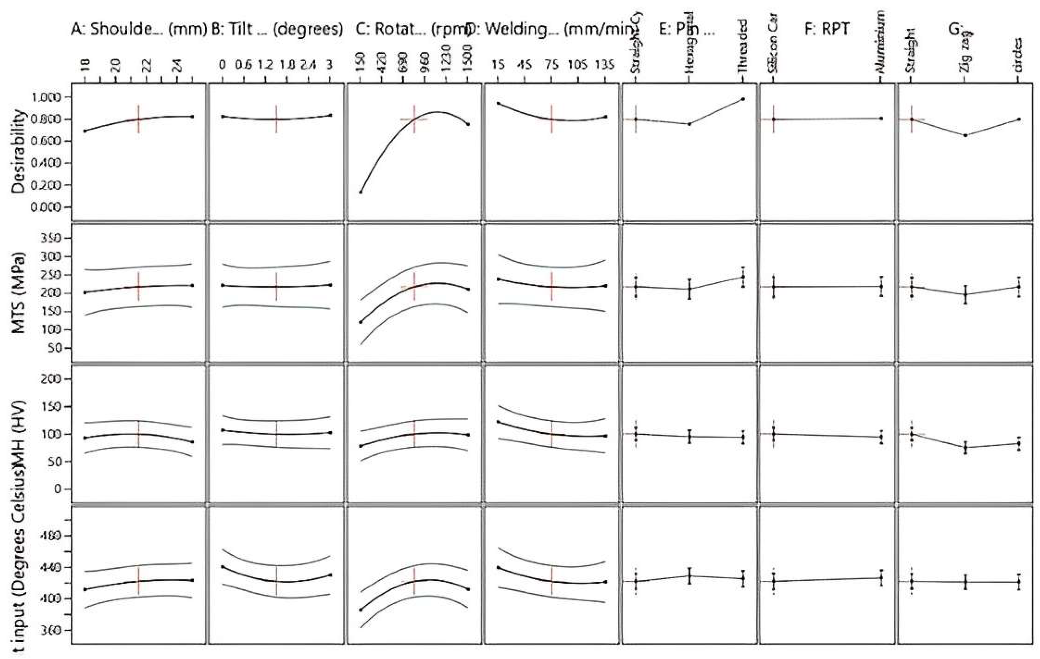
4.2. Using Design-Expert Software to Form the Multi-Objective Mathematical Model

The multi-objective model was used in this study to optimize three objectives simultaneously; optimizing one objective function has an influence on the other objectives. As can be seen from the data presented in Table 7, in experiment number 5, the UTS was at the maximum but also increased the heat input that occurred during the welding process. The purpose of this research was to reduce the temperature effect so that the change in microstructure in the welding area would be kept to a minimum. In experiment 24, we can see that the heat was minimized. The heat in experiment 24 represented a decrease of 12.69% from that in experiment 5; however, the UTS was reduced by 48.85%, which is relatively high. Consequently, we cannot maximize a single objective while retaining the intactness of other objectives. In the multi-objective optimization model that we built for this study, MoDE was carried out by utilizing the mathematical model acquired using the Design-Expert v. 13 software. The mathematical model was formulated as shown in the following section.

4.2.1. The Mathematical Model for Ultimate Tensile Strength $({\mathrm{U}\mathrm{T}\mathrm{S}}^{\mathrm{M}\mathrm{o}\mathrm{d}\mathrm{e}\mathrm{l}})$

Software Design-Expert v. 13 was used to generate a mathematical model, demonstrating the association between the variable values based on the data in Table 7. As the p-values of the quadratic model were less than 0.05 and the model was statistically significant with a 95% confidence interval, the ANOVA findings obtained for UTS indicated that the model’s forms were acceptable for utilization as mathematical models. The mathematical model had a coefficient of determination (R2) of 95.04% due to the influence of the variables, and the revised coefficient (adjusted R2) was greater than 71.72%, confirming that the regression model had a correct format for the above UTS response, as shown in

Table 8. The ANOVA results for the UTS response obtained using the Design-Expert v. 13 software.

Source of Variation	Sum of Squares	DF	Mean Squares	F-Value	p-Value
Model	154,900	47	3295.64	4.08	0.0105
Linear	45,075.78	43	1048.27	0.9314	0.6116
Residual Error	8085.27	10	808.53
Lack-of-Fit	2458.11	5	491.62	0.4368	0.8077
Pure Error	5627.16	5	1125.43
Total	163,000	57
R-sq = 95.04%, R-sq (adj) = 71.72%

. The models used for the UTS characteristics were based on Equations (14)–(31).

$$\begin{array}{cc}\mathrm{StC}\_\mathrm{SiC}\_\mathrm{S}=\hfill & -88.30498+19.22792\mathrm{SD}-44.37324\mathrm{T}\mathrm{A}+0.250058\mathrm{R}\mathrm{t}\mathrm{S}-0.585186\mathrm{W}\mathrm{S}\hfill \\ & +2.08588\mathrm{S}\mathrm{D}\times \mathrm{T}\mathrm{A}+0.000624\mathrm{S}\mathrm{D}\times \mathrm{R}\mathrm{t}\mathrm{S}-0.001537\mathrm{S}\mathrm{D}\times \mathrm{W}\mathrm{S}-0.006381\mathrm{T}\mathrm{A}\times \mathrm{R}\mathrm{t}\mathrm{S}\hfill \\ & -0.010422\mathrm{T}\mathrm{A}\times \mathrm{W}\mathrm{S}-0.000032\mathrm{R}\mathrm{t}\mathrm{S}\times \mathrm{W}\mathrm{S}-0.467021{\mathrm{S}\mathrm{D}}^2+2.00253{\mathrm{T}\mathrm{A}}^2\hfill \\ & -0.000112{\mathrm{R}\mathrm{t}\mathrm{S}}^2+0.003393{\mathrm{W}\mathrm{S}}^2\hfill \end{array}$$

(14)

$$\begin{array}{cc}\mathrm{StC}\_\mathrm{SiC}\_\mathrm{Z}=\hfill & -6.11488+16.52802\mathrm{SD}-61.10962\mathrm{T}\mathrm{A}+0.241531\mathrm{R}\mathrm{t}\mathrm{S}-0.761831\mathrm{W}\mathrm{S}\hfill \\ & +2.08588\mathrm{S}\mathrm{D}\times \mathrm{T}\mathrm{A}+0.000624\mathrm{S}\mathrm{D}\times \mathrm{R}\mathrm{t}\mathrm{S}-0.001537\mathrm{S}\mathrm{D}\times \mathrm{W}\mathrm{S}-0.006381\mathrm{T}\mathrm{A}\times \mathrm{R}\mathrm{t}\mathrm{S}\hfill \\ & -0.010422\mathrm{T}\mathrm{A}\times \mathrm{W}\mathrm{S}-0.000032\mathrm{R}\mathrm{t}\mathrm{S}\times \mathrm{W}\mathrm{S}-0.467021{\mathrm{S}\mathrm{D}}^2+2.00253{\mathrm{T}\mathrm{A}}^2\hfill \\ & -0.000112{\mathrm{R}\mathrm{t}\mathrm{S}}^2+0.003393\mathrm{W}\mathrm{S}\hfill \end{array}$$

(15)

$$\begin{array}{cc}\mathrm{StC}\_\mathrm{SiC}\_\mathrm{C}=\hfill & -14.59844+16.74932\mathrm{SD}-47.53187\mathrm{T}\mathrm{A}+0.245462\mathrm{R}\mathrm{t}\mathrm{S}-0.742827\mathrm{W}\mathrm{S}\hfill \\ & +2.08588\mathrm{S}\mathrm{D}\times \mathrm{T}\mathrm{A}+0.000624\mathrm{S}\mathrm{D}\times \mathrm{R}\mathrm{t}\mathrm{S}-0.001537\mathrm{S}\mathrm{D}\times \mathrm{W}\mathrm{S}-0.006381\mathrm{T}\mathrm{A}\times \mathrm{R}\mathrm{t}\mathrm{S}\hfill \\ & -0.010422\mathrm{T}\mathrm{A}\times \mathrm{W}\mathrm{S}-0.000032\mathrm{R}\mathrm{t}\mathrm{S}\times \mathrm{W}\mathrm{S}-0.467021{\mathrm{S}\mathrm{D}}^2+2.00253{\mathrm{T}\mathrm{A}}^2\hfill \\ & -0.000112{\mathrm{R}\mathrm{t}\mathrm{S}}^2+0.003393{\mathrm{W}\mathrm{S}}^2\hfill \end{array}$$

(16)

$$\begin{array}{cc}\mathrm{StC}\_\mathrm{AO}\_\mathrm{S}=\hfill & -50.59953+17.00317\mathrm{SD}-45.46861\mathrm{T}\mathrm{A}+0.262807\mathrm{R}\mathrm{t}\mathrm{S}-0.553276\mathrm{W}\mathrm{S}\hfill \\ & +2.08588\mathrm{S}\mathrm{D}\times \mathrm{T}\mathrm{A}+0.000624\mathrm{S}\mathrm{D}\times \mathrm{R}\mathrm{t}\mathrm{S}-0.001537\mathrm{S}\mathrm{D}\times \mathrm{W}\mathrm{S}-0.006381\mathrm{T}\mathrm{A}\times \mathrm{R}\mathrm{t}\mathrm{S}\hfill \\ & -0.010422\mathrm{T}\mathrm{A}\times \mathrm{W}\mathrm{S}-0.000032\mathrm{R}\mathrm{t}\mathrm{S}\times \mathrm{W}\mathrm{S}-0.467021{\mathrm{S}\mathrm{D}}^2+2.00253{\mathrm{T}\mathrm{A}}^2\hfill \\ & -0.000112{\mathrm{R}\mathrm{t}\mathrm{S}}^2+0.003393{\mathrm{W}\mathrm{S}}^2\hfill \end{array}$$

(17)

$$\begin{array}{cc}\mathrm{StC}\_\mathrm{AO}\_\mathrm{Z}=\hfill & 43.15132+14.30326\mathrm{SD}-62.20499\mathrm{T}\mathrm{A}+0.254280\mathrm{R}\mathrm{t}\mathrm{S}-0.729921\mathrm{W}\mathrm{S}\hfill \\ & +2.08588\mathrm{S}\mathrm{D}\times \mathrm{T}\mathrm{A}+0.000624\mathrm{S}\mathrm{D}\times \mathrm{R}\mathrm{t}\mathrm{S}-0.001537\mathrm{S}\mathrm{D}\times \mathrm{W}\mathrm{S}-0.006381\mathrm{T}\mathrm{A}\times \mathrm{R}\mathrm{t}\mathrm{S}\hfill \\ & -0.010422\mathrm{T}\mathrm{A}\times \mathrm{W}\mathrm{S}-0.000032\mathrm{R}\mathrm{t}\mathrm{S}\times \mathrm{W}\mathrm{S}-0.467021{\mathrm{S}\mathrm{D}}^2+2.00253{\mathrm{T}\mathrm{A}}^2\hfill \\ & -0.000112{\mathrm{R}\mathrm{t}\mathrm{S}}^2+0.003393{\mathrm{W}\mathrm{S}}^2\hfill \end{array}$$

(18)

$$\begin{array}{cc}\mathrm{StC}\_\mathrm{AO}\_\mathrm{C}=\hfill & 21.80674+14.52456\mathrm{SD}-48.62724\mathrm{T}\mathrm{A}+0.258211\mathrm{R}\mathrm{t}\mathrm{S}-0.710917\mathrm{W}\mathrm{S}\hfill \\ & +2.08588\mathrm{S}\mathrm{D}\times \mathrm{T}\mathrm{A}+0.000624\mathrm{S}\mathrm{D}\times \mathrm{R}\mathrm{t}\mathrm{S}-0.001537\mathrm{S}\mathrm{D}\times \mathrm{W}\mathrm{S}-0.006381\mathrm{T}\mathrm{A}\times \mathrm{R}\mathrm{t}\mathrm{S}\hfill \\ & -0.010422\mathrm{T}\mathrm{A}\times \mathrm{W}\mathrm{S}-0.000032\mathrm{R}\mathrm{t}\mathrm{S}\times \mathrm{W}\mathrm{S}-0.467021{\mathrm{S}\mathrm{D}}^2+2.00253{\mathrm{T}\mathrm{A}}^2\hfill \\ & -0.000112{\mathrm{R}\mathrm{t}\mathrm{S}}^2+0.003393{\mathrm{W}\mathrm{S}}^2\hfill \end{array}$$

(19)

$$\begin{array}{cc}\mathrm{HC}\_\mathrm{SiC}\_\mathrm{S}=\hfill & -167.32310+20.92138\mathrm{SD}-39.29650\mathrm{T}\mathrm{A}+0.263002\mathrm{R}\mathrm{t}\mathrm{S}-0.341700\mathrm{W}\mathrm{S}\hfill \\ & +2.08588\mathrm{S}\mathrm{D}\times \mathrm{T}\mathrm{A}+0.000624\mathrm{S}\mathrm{D}\times \mathrm{R}\mathrm{t}\mathrm{S}-0.001537\mathrm{S}\mathrm{D}\times \mathrm{W}\mathrm{S}-0.006381\mathrm{T}\mathrm{A}\times \mathrm{R}\mathrm{t}\mathrm{S}\hfill \\ & -0.010422\mathrm{T}\mathrm{A}\times \mathrm{W}\mathrm{S}-0.000032\mathrm{R}\mathrm{t}\mathrm{S}\times \mathrm{W}\mathrm{S}-0.467021{\mathrm{S}\mathrm{D}}^2+2.00253{\mathrm{T}\mathrm{A}}^2\hfill \\ & -0.000112{\mathrm{R}\mathrm{t}\mathrm{S}}^2+0.003393{\mathrm{W}\mathrm{S}}^2\hfill \end{array}$$

(20)

$$\begin{array}{cc}\mathrm{HC}\_\mathrm{SiC}\_\mathrm{Z}=\hfill & -64.48001+18.22148\mathrm{SD}-56.03288\mathrm{T}\mathrm{A}+0.254474\mathrm{R}\mathrm{t}\mathrm{S}-0.518345\mathrm{W}\mathrm{S}\hfill \\ & +2.08588\mathrm{S}\mathrm{D}\times \mathrm{T}\mathrm{A}+0.000624\mathrm{S}\mathrm{D}\times \mathrm{R}\mathrm{t}\mathrm{S}-0.001537\mathrm{S}\mathrm{D}\times \mathrm{W}\mathrm{S}-0.006381\mathrm{T}\mathrm{A}\times \mathrm{R}\mathrm{t}\mathrm{S}\hfill \\ & -0.010422\mathrm{T}\mathrm{A}\times \mathrm{W}\mathrm{S}-0.000032\mathrm{R}\mathrm{t}\mathrm{S}\times \mathrm{W}\mathrm{S}-0.467021{\mathrm{S}\mathrm{D}}^2+2.00253{\mathrm{T}\mathrm{A}}^2\hfill \\ & -0.000112{\mathrm{R}\mathrm{t}\mathrm{S}}^2+0.003393{\mathrm{W}\mathrm{S}}^2\hfill \end{array}$$

(21)

$$\begin{array}{cc}\mathrm{HC}\_\mathrm{SiC}\_\mathrm{C}=\hfill & -81.12537+18.44278\mathrm{SD}-42.45513\mathrm{T}\mathrm{A}+0.258406\mathrm{R}\mathrm{t}\mathrm{S}-0.499341\mathrm{W}\mathrm{S}\hfill \\ & +2.08588\mathrm{S}\mathrm{D}\times \mathrm{T}\mathrm{A}+0.000624\mathrm{S}\mathrm{D}\times \mathrm{R}\mathrm{t}\mathrm{S}-0.001537\mathrm{S}\mathrm{D}\times \mathrm{W}\mathrm{S}-0.006381\mathrm{T}\mathrm{A}\times \mathrm{R}\mathrm{t}\mathrm{S}\hfill \\ & -0.010422\mathrm{T}\mathrm{A}\times \mathrm{W}\mathrm{S}-0.000032\mathrm{R}\mathrm{t}\mathrm{S}\times \mathrm{W}\mathrm{S}-0.467021{\mathrm{S}\mathrm{D}}^2+2.00253{\mathrm{T}\mathrm{A}}^2\hfill \\ & -0.000112{\mathrm{R}\mathrm{t}\mathrm{S}}^2+0.003393{\mathrm{W}\mathrm{S}}^2\hfill \end{array}$$

(22)

$$\begin{array}{cc}\mathrm{HC}\_\mathrm{AO}\_\mathrm{S}=\hfill & -126.74310+18.69663\mathrm{SD}-40.39187\mathrm{T}\mathrm{A}+0.275751\mathrm{R}\mathrm{t}\mathrm{S}-0.309790\mathrm{W}\mathrm{S}\hfill \\ & +2.08588\mathrm{S}\mathrm{D}\times \mathrm{T}\mathrm{A}+0.000624\mathrm{S}\mathrm{D}\times \mathrm{R}\mathrm{t}\mathrm{S}-0.001537\mathrm{S}\mathrm{D}\times \mathrm{W}\mathrm{S}-0.006381\mathrm{T}\mathrm{A}\times \mathrm{R}\mathrm{t}\mathrm{S}\hfill \\ & -0.010422\mathrm{T}\mathrm{A}\times \mathrm{W}\mathrm{S}-0.000032\mathrm{R}\mathrm{t}\mathrm{S}\times \mathrm{W}\mathrm{S}-0.467021{\mathrm{S}\mathrm{D}}^2+2.00253{\mathrm{T}\mathrm{A}}^2\hfill \\ & -0.000112{\mathrm{R}\mathrm{t}\mathrm{S}}^2+0.003393{\mathrm{W}\mathrm{S}}^2\hfill \end{array}$$

(23)

$$\begin{array}{cc}\mathrm{HC}\_\mathrm{AO}\_\mathrm{Z}=\hfill & -12.33928+15.99672\mathrm{SD}-57.12825\mathrm{T}\mathrm{A}+0.267223\mathrm{R}\mathrm{t}\mathrm{S}-0.486435\mathrm{W}\mathrm{S}\hfill \\ & +2.08588\mathrm{S}\mathrm{D}\times \mathrm{T}\mathrm{A}+0.000624\mathrm{S}\mathrm{D}\times \mathrm{R}\mathrm{t}\mathrm{S}-0.001537\mathrm{S}\mathrm{D}\times \mathrm{W}\mathrm{S}-0.006381\mathrm{T}\mathrm{A}\times \mathrm{R}\mathrm{t}\mathrm{S}\hfill \\ & -0.010422\mathrm{T}\mathrm{A}\times \mathrm{W}\mathrm{S}-0.000032\mathrm{R}\mathrm{t}\mathrm{S}\times \mathrm{W}\mathrm{S}-0.467021{\mathrm{S}\mathrm{D}}^2+2.00253{\mathrm{T}\mathrm{A}}^2\hfill \\ & -0.000112{\mathrm{R}\mathrm{t}\mathrm{S}}^2+0.003393{\mathrm{W}\mathrm{S}}^2\hfill \end{array}$$

(24)

$$\begin{array}{cc}\mathrm{HC}\_\mathrm{AO}\_\mathrm{C}=\hfill & -41.84565+16.21802\mathrm{SD}-43.55050\mathrm{T}\mathrm{A}+0.271155\mathrm{R}\mathrm{t}\mathrm{S}-0.467431\mathrm{W}\mathrm{S}\hfill \\ & +2.08588\mathrm{S}\mathrm{D}\times \mathrm{T}\mathrm{A}+0.000624\mathrm{S}\mathrm{D}\times \mathrm{R}\mathrm{t}\mathrm{S}-0.001537\mathrm{S}\mathrm{D}\times \mathrm{W}\mathrm{S}-0.006381\mathrm{T}\mathrm{A}\times \mathrm{R}\mathrm{t}\mathrm{S}\hfill \\ & -0.010422\mathrm{T}\mathrm{A}\times \mathrm{W}\mathrm{S}-0.000032\mathrm{R}\mathrm{t}\mathrm{S}\times \mathrm{W}\mathrm{S}-0.467021{\mathrm{S}\mathrm{D}}^2+2.00253{\mathrm{T}\mathrm{A}}^2\hfill \\ & -0.000112{\mathrm{R}\mathrm{t}\mathrm{S}}^2+0.003393{\mathrm{W}\mathrm{S}}^2\hfill \end{array}$$

(25)

$$\begin{array}{cc}\mathrm{TC}\_\mathrm{SiC}\_\mathrm{S}=\hfill & -120.63139+19.85389\mathrm{SD}-26.74226\mathrm{T}\mathrm{A}+0.252933\mathrm{R}\mathrm{t}\mathrm{S}-0.359441\mathrm{W}\mathrm{S}\hfill \\ & +2.08588\mathrm{S}\mathrm{D}\times \mathrm{T}\mathrm{A}+0.000624\mathrm{S}\mathrm{D}\times \mathrm{R}\mathrm{t}\mathrm{S}-0.001537\mathrm{S}\mathrm{D}\times \mathrm{W}\mathrm{S}-0.006381\mathrm{T}\mathrm{A}\times \mathrm{R}\mathrm{t}\mathrm{S}\hfill \\ & -0.010422\mathrm{T}\mathrm{A}\times \mathrm{W}\mathrm{S}-0.000032\mathrm{R}\mathrm{t}\mathrm{S}\times \mathrm{W}\mathrm{S}-0.467021{\mathrm{S}\mathrm{D}}^2+2.00253{\mathrm{T}\mathrm{A}}^2\hfill \\ & -0.000112{\mathrm{R}\mathrm{t}\mathrm{S}}^2+0.003393{\mathrm{W}\mathrm{S}}^2\hfill \end{array}$$

(26)

$$\begin{array}{cc}\mathrm{TC}\_\mathrm{SiC}\_\mathrm{Z}=\hfill & -44.58598+17.15399\mathrm{SD}-43.47864\mathrm{T}\mathrm{A}+0.244405\mathrm{R}\mathrm{t}\mathrm{S}-0.536086\mathrm{W}\mathrm{S}\hfill \\ & +2.08588\mathrm{S}\mathrm{D}\times \mathrm{T}\mathrm{A}+0.000624\mathrm{S}\mathrm{D}\times \mathrm{R}\mathrm{t}\mathrm{S}-0.001537\mathrm{S}\mathrm{D}\times \mathrm{W}\mathrm{S}-0.006381\mathrm{T}\mathrm{A}\times \mathrm{R}\mathrm{t}\mathrm{S}\hfill \\ & -0.010422\mathrm{T}\mathrm{A}\times \mathrm{W}\mathrm{S}-0.000032\mathrm{R}\mathrm{t}\mathrm{S}\times \mathrm{W}\mathrm{S}-0.467021{\mathrm{S}\mathrm{D}}^2+2.00253{\mathrm{T}\mathrm{A}}^2\hfill \\ & -0.000112{\mathrm{R}\mathrm{t}\mathrm{S}}^2+0.003393{\mathrm{W}\mathrm{S}}^2\hfill \end{array}$$

(27)

$$\begin{array}{cc}\mathrm{TC}\_\mathrm{SiC}\_\mathrm{C}=\hfill & -62.50272+17.37529\mathrm{SD}-29.90090\mathrm{T}\mathrm{A}+0.248336\mathrm{R}\mathrm{t}\mathrm{S}-0.517082\mathrm{W}\mathrm{S}\hfill \\ & +2.08588\mathrm{S}\mathrm{D}\times \mathrm{T}\mathrm{A}+0.000624\mathrm{S}\mathrm{D}\times \mathrm{R}\mathrm{t}\mathrm{S}-0.001537\mathrm{S}\mathrm{D}\times \mathrm{W}\mathrm{S}-0.006381\mathrm{T}\mathrm{A}\times \mathrm{R}\mathrm{t}\mathrm{S}\hfill \\ & -0.010422\mathrm{T}\mathrm{A}\times \mathrm{W}\mathrm{S}-0.000032\mathrm{R}\mathrm{t}\mathrm{S}\times \mathrm{W}\mathrm{S}-0.467021{\mathrm{S}\mathrm{D}}^2+2.00253{\mathrm{T}\mathrm{A}}^2\hfill \\ & -0.000112{\mathrm{R}\mathrm{t}\mathrm{S}}^2+0.003393{\mathrm{W}\mathrm{S}}^2\hfill \end{array}$$

(28)

$$\begin{array}{cc}\mathrm{TC}\_\mathrm{AO}\_\mathrm{S}=\hfill & -95.24823+17.62914\mathrm{SD}-27.83764\mathrm{T}\mathrm{A}+0.265682\mathrm{R}\mathrm{t}\mathrm{S}-0.327532\mathrm{W}\mathrm{S}\hfill \\ & +2.08588\mathrm{S}\mathrm{D}\times \mathrm{T}\mathrm{A}+0.000624\mathrm{S}\mathrm{D}\times \mathrm{R}\mathrm{t}\mathrm{S}-0.001537\mathrm{S}\mathrm{D}\times \mathrm{W}\mathrm{S}-0.006381\mathrm{T}\mathrm{A}\times \mathrm{R}\mathrm{t}\mathrm{S}\hfill \\ & -0.010422\mathrm{T}\mathrm{A}\times \mathrm{W}\mathrm{S}-0.000032\mathrm{R}\mathrm{t}\mathrm{S}\times \mathrm{W}\mathrm{S}-0.467021{\mathrm{S}\mathrm{D}}^2+2.00253{\mathrm{T}\mathrm{A}}^2\hfill \\ & -0.000112{\mathrm{R}\mathrm{t}\mathrm{S}}^2+0.003393\mathrm{W}\mathrm{S}\hfill \end{array}$$

(29)

$$\begin{array}{cc}\mathrm{TC}\_\mathrm{AO}\_\mathrm{Z}=\hfill & -7.64208+14.92923\mathrm{SD}-44.57401\mathrm{T}\mathrm{A}+0.257154\mathrm{R}\mathrm{t}\mathrm{S}-0.504177\mathrm{W}\mathrm{S}\hfill \\ & +2.08588\mathrm{S}\mathrm{D}\times \mathrm{T}\mathrm{A}+0.000624\mathrm{S}\mathrm{D}\times \mathrm{R}\mathrm{t}\mathrm{S}-0.001537\mathrm{S}\mathrm{D}\times \mathrm{W}\mathrm{S}-0.006381\mathrm{T}\mathrm{A}\times \mathrm{R}\mathrm{t}\mathrm{S}\hfill \\ & -0.010422\mathrm{T}\mathrm{A}\times \mathrm{W}\mathrm{S}-0.000032\mathrm{R}\mathrm{t}\mathrm{S}\times \mathrm{W}\mathrm{S}-0.467021{\mathrm{S}\mathrm{D}}^2+2.00253{\mathrm{T}\mathrm{A}}^2\hfill \\ & -0.000112{\mathrm{R}\mathrm{t}\mathrm{S}}^2+0.003393{\mathrm{W}\mathrm{S}}^2\hfill \end{array}$$

(30)

$$\begin{array}{cc}\mathrm{TC}\_\mathrm{AO}\_\mathrm{C}=\hfill & -38.41983+15.15053\mathrm{SD}-30.99627\mathrm{T}\mathrm{A}+0.261085\mathrm{R}\mathrm{t}\mathrm{S}-0.485173\mathrm{W}\mathrm{S}\hfill \\ & +2.08588\mathrm{S}\mathrm{D}\times \mathrm{T}\mathrm{A}+0.000624\mathrm{S}\mathrm{D}\times \mathrm{R}\mathrm{t}\mathrm{S}-0.001537\mathrm{S}\mathrm{D}\times \mathrm{W}\mathrm{S}-0.006381\mathrm{T}\mathrm{A}\times \mathrm{R}\mathrm{t}\mathrm{S}\hfill \\ & -0.010422\mathrm{T}\mathrm{A}\times \mathrm{W}\mathrm{S}-0.000032\mathrm{R}\mathrm{t}\mathrm{S}\times \mathrm{W}\mathrm{S}-0.467021{\mathrm{S}\mathrm{D}}^2+2.00253{\mathrm{T}\mathrm{A}}^2\hfill \\ & -0.000112{\mathrm{R}\mathrm{t}\mathrm{S}}^2+0.003393{\mathrm{W}\mathrm{S}}^2\hfill \end{array}$$

(31)

SD, TA, RtS, and WS represent the shoulder diameter (mm), tilt angle (degrees), rotation speed (rpm), and welding speed (mm/min), respectively.

Equations (14)–(31) were formulated from the data shown in Table 7 using the Design-Expert v. 13 software for determining the response of UTS. The categories include three pin-type variables, two reinforcement particle type variables, and three tool pin movement types. The processing software can generate 18 equations, and each equation is divided into details as shown in

Table 9. Details of the models generated by Design-Expert v. 13 software.

Model Name	Detail	Model Name	Detail
StC_SiC_S	Pin Type: Straight Cylindrical	HC_AO_S	Pin Type: Hexagonal
	Particles Type: Silicon Carbide		Particles Type: Aluminum Oxide
	Tool Pin Movement: Straight		Tool Pin Movement: Straight
StC_SiC_Z	Pin Type: Straight Cylindrical	HC_AO_Z	Pin Type: Hexagonal
	Particles Type: Silicon Carbide		Particles Type: Aluminum Oxide
	Tool Pin Movement: Zig Zag		Tool Pin Movement: Zig Zag
StC_SiC_C	Pin Type: Straight Cylindrical	HC_AO_C	Pin Type: Hexagonal
	Particles Type: Silicon Carbide		Particles Type: Aluminum Oxide
	Tool Pin Movement: Circles		Tool Pin Movement: Circles
StC_AO_S	Pin Type: Straight Cylindrical	TC_SiC_S	Pin Type: Threaded
	Particles Type: Aluminum Oxide		Particles Type: Silicon Carbide
	Tool Pin Movement: Straight		Tool Pin Movement: Straight
StC_AO_Z	Pin Type: Straight Cylindrical	TC_SiC_Z	Pin Type: Threaded
	Particles Type: Aluminum Oxide		Particles Type: Silicon Carbide
	Tool Pin Movement: Zig Zag		Tool Pin Movement: Zig Zag
StC_AO_C	Pin Type: Straight Cylindrical	TC_SiC_C	Pin Type: Threaded
	Particles Type: Aluminum Oxide		Particles Type: Silicon Carbide
	Tool Pin Movement: Circles		Tool Pin Movement: Circles
HC_SiC_S	Pin Type: Hexagonal	TC_AO_S	Pin Type: Threaded
	Particles Type: Silicon Carbide		Particles Type: Aluminum Oxide
	Tool Pin Movement: Straight		Tool Pin Movement: Straight
HC_SiC_Z	Pin Type: Hexagonal	TC_AO_Z	Pin Type: Threaded
	Particles Type: Silicon Carbide		Particles Type: Aluminum Oxide
	Tool Pin Movement: Zig Zag		Tool Pin Movement: Zig Zag
HC_SiC_C	Pin Type: Hexagonal	TC_AO_C	Pin Type: Threaded
	Particles Type: Silicon Carbide		Particles Type: Aluminum Oxide
	Tool Pin Movement: Circles		Tool Pin Movement: Circles

.

4.2.2. The Mathematical Model for Maximum Hardness (${\mathrm{M}\mathrm{H}}^{\mathrm{M}\mathrm{o}\mathrm{d}\mathrm{e}\mathrm{l}}$)

The ANOVA findings obtained for MH indicated that the model’s forms were acceptable for utilization as mathematical models, as the p-values of the quadratic model were less than 0.05 and the model was statistically significant with a 95% confidence range. The mathematical model had a coefficient of determination (R2) equal to 94.30% due to the influence of variables, and the revised coefficient (adjusted R2) was greater than 67.53%, confirming that the regression model had the correct format for the above MH response, as illustrated in

Table 10. The ANOVA results for the MH response obtained using the Design-Expert v. 13 software.

Source of Variation	Sum of Squares	DF	Mean Squares	F-Value	p-Value
Model	26,858.81	47	571.46	3.52	0.0182
Linear	10,836.28	43	252.01	1.01	0.5622
Residual Error	1622.57	10	162.26
Lack-of-Fit	380.95	5	76.19	0.3068	0.8897
Pure Error	1241.62	5	248.32
Total	28,481.38	57
R-sq = 94.30%, R-sq (adj) = 67.53%

. Equations (32)–(49) were used as the models for the MH.

$$\begin{array}{cc}\mathrm{StC}\_\mathrm{SiC}\_\mathrm{S}=\hfill & -184.48143+33.15735\mathrm{SD}-44.90477\mathrm{T}\mathrm{A}+0.027221\mathrm{R}\mathrm{t}\mathrm{S}-0.934965\mathrm{W}\mathrm{S}\hfill \\ & +1.57366\mathrm{S}\mathrm{D}\times \mathrm{T}\mathrm{A}+0.001149\mathrm{S}\mathrm{D}\times \mathrm{R}\mathrm{t}\mathrm{S}+0.009940\mathrm{S}\mathrm{D}\times \mathrm{W}\mathrm{S}-0.000080\mathrm{T}\mathrm{A}\times \mathrm{R}\mathrm{t}\mathrm{S}\hfill \\ & +0.042159\mathrm{T}\mathrm{A}\times \mathrm{W}\mathrm{S}+0.000069\mathrm{R}\mathrm{t}\mathrm{S}\times \mathrm{W}\mathrm{S}-0.889454{\mathrm{S}\mathrm{D}}^2+2.14136{\mathrm{T}\mathrm{A}}^2\hfill \\ & -0.000025{\mathrm{R}\mathrm{t}\mathrm{S}}^2+0.002610{\mathrm{W}\mathrm{S}}^2\hfill \end{array}$$

(32)

$$\begin{array}{cc}\mathrm{StC}\_\mathrm{SiC}\_\mathrm{Z}=\hfill & -176.55800+32.40781\mathrm{SD}-51.85869\mathrm{T}\mathrm{A}+0.029131\mathrm{R}\mathrm{t}\mathrm{S}-1.03611\mathrm{W}\mathrm{S}\hfill \\ & +1.57366\mathrm{S}\mathrm{D}\times \mathrm{T}\mathrm{A}+0.001149\mathrm{S}\mathrm{D}\times \mathrm{R}\mathrm{t}\mathrm{S}+0.009940\mathrm{S}\mathrm{D}\times \mathrm{W}\mathrm{S}-0.000080\mathrm{T}\mathrm{A}\times \mathrm{R}\mathrm{t}\mathrm{S}\hfill \\ & +0.042159\mathrm{T}\mathrm{A}\times \mathrm{W}\mathrm{S}+0.000069\mathrm{R}\mathrm{t}\mathrm{S}\times \mathrm{W}\mathrm{S}-0.889454{\mathrm{S}\mathrm{D}}^2+2.14136{\mathrm{T}\mathrm{A}}^2\hfill \\ & -0.000025{\mathrm{R}\mathrm{t}\mathrm{S}}^2+0.002610{\mathrm{W}\mathrm{S}}^2\hfill \end{array}$$

(33)

$$\begin{array}{cc}\mathrm{StC}\_\mathrm{SiC}\_\mathrm{C}=\hfill & -205.50651+33.20038\mathrm{SD}-45.91115\mathrm{T}\mathrm{A}+0.031632\mathrm{R}\mathrm{t}\mathrm{S}-0.927271\mathrm{W}\mathrm{S}\hfill \\ & +1.57366\mathrm{S}\mathrm{D}\times \mathrm{T}\mathrm{A}+0.001149\mathrm{S}\mathrm{D}\times \mathrm{R}\mathrm{t}\mathrm{S}+0.009940\mathrm{S}\mathrm{D}\times \mathrm{W}\mathrm{S}-0.000080\mathrm{T}\mathrm{A}\times \mathrm{R}\mathrm{t}\mathrm{S}\hfill \\ & +0.042159\mathrm{T}\mathrm{A}\times \mathrm{W}\mathrm{S}+0.000069\mathrm{R}\mathrm{t}\mathrm{S}\times \mathrm{W}\mathrm{S}-0.889454{\mathrm{S}\mathrm{D}}^2+2.14136{\mathrm{T}\mathrm{A}}^2\hfill \\ & -0.000025{\mathrm{R}\mathrm{t}\mathrm{S}}^2+0.002610{\mathrm{W}\mathrm{S}}^2\hfill \end{array}$$

(34)

$$\begin{array}{cc}\mathrm{StC}\_\mathrm{AO}\_\mathrm{S}=\hfill & -193.01865+32.44733\mathrm{SD}-44.55763\mathrm{T}\mathrm{A}+0.040812\mathrm{R}\mathrm{t}\mathrm{S}-0.844855\mathrm{W}\mathrm{S}\hfill \\ & +1.57366\mathrm{S}\mathrm{D}\times \mathrm{T}\mathrm{A}+0.001149\mathrm{S}\mathrm{D}\times \mathrm{R}\mathrm{t}\mathrm{S}+0.009940\mathrm{S}\mathrm{D}\times \mathrm{W}\mathrm{S}-0.000080\mathrm{T}\mathrm{A}\times \mathrm{R}\mathrm{t}\mathrm{S}\hfill \\ & +0.042159\mathrm{T}\mathrm{A}\times \mathrm{W}\mathrm{S}+0.000069\mathrm{R}\mathrm{t}\mathrm{S}\times \mathrm{W}\mathrm{S}-0.889454{\mathrm{S}\mathrm{D}}^2+2.14136{\mathrm{T}\mathrm{A}}^2\hfill \\ & -0.000025{\mathrm{R}\mathrm{t}\mathrm{S}}^2+0.002610{\mathrm{W}\mathrm{S}}^2\hfill \end{array}$$

(35)

$$\begin{array}{cc}\mathrm{StC}\_\mathrm{AO}\_\mathrm{Z}=\hfill & -174.43668+31.69779\mathrm{SD}-51.51155\mathrm{T}\mathrm{A}+0.042722\mathrm{R}\mathrm{t}\mathrm{S}-0.945997\mathrm{W}\mathrm{S}\hfill \\ & +1.57366\mathrm{S}\mathrm{D}\times \mathrm{T}\mathrm{A}+0.001149\mathrm{S}\mathrm{D}\times \mathrm{R}\mathrm{t}\mathrm{S}+0.009940\mathrm{S}\mathrm{D}\times \mathrm{W}\mathrm{S}-0.000080\mathrm{T}\mathrm{A}\times \mathrm{R}\mathrm{t}\mathrm{S}\hfill \\ & +0.042159\mathrm{T}\mathrm{A}\times \mathrm{W}\mathrm{S}+0.000069\mathrm{R}\mathrm{t}\mathrm{S}\times \mathrm{W}\mathrm{S}-0.889454{\mathrm{S}\mathrm{D}}^2+2.14136{\mathrm{T}\mathrm{A}}^2\hfill \\ & -0.000025{\mathrm{R}\mathrm{t}\mathrm{S}}^2+0.002610{\mathrm{W}\mathrm{S}}^2\hfill \end{array}$$

(36)

$$\begin{array}{cc}\mathrm{StC}\_\mathrm{AO}\_\mathrm{C}=\hfill & -205.21203+32.49036\mathrm{SD}-45.56402\mathrm{T}\mathrm{A}+0.045223\mathrm{R}\mathrm{t}\mathrm{S}-0.837162\mathrm{W}\mathrm{S}\hfill \\ & +1.57366\mathrm{S}\mathrm{D}\times \mathrm{T}\mathrm{A}+0.001149\mathrm{S}\mathrm{D}\times \mathrm{R}\mathrm{t}\mathrm{S}+0.009940\mathrm{S}\mathrm{D}\times \mathrm{W}\mathrm{S}-0.000080\mathrm{T}\mathrm{A}\times \mathrm{R}\mathrm{t}\mathrm{S}\hfill \\ & +0.042159\mathrm{T}\mathrm{A}\times \mathrm{W}\mathrm{S}+0.000069\mathrm{R}\mathrm{t}\mathrm{S}\times \mathrm{W}\mathrm{S}-0.889454{\mathrm{S}\mathrm{D}}^2+2.14136{\mathrm{T}\mathrm{A}}^2\hfill \\ & -0.000025{\mathrm{R}\mathrm{t}\mathrm{S}}^2+0.002610{\mathrm{W}\mathrm{S}}^2\hfill \end{array}$$

(37)

$$\begin{array}{cc}\mathrm{HC}\_\mathrm{SiC}\_\mathrm{S}=\hfill & -241.36155+34.71881\mathrm{SD}-44.79972\mathrm{T}\mathrm{A}+0.031430\mathrm{R}\mathrm{t}\mathrm{S}-0.737514\mathrm{W}\mathrm{S}\hfill \\ & +1.57366\mathrm{S}\mathrm{D}\times \mathrm{T}\mathrm{A}+0.001149\mathrm{S}\mathrm{D}\times \mathrm{R}\mathrm{t}\mathrm{S}+0.009940\mathrm{S}\mathrm{D}\times \mathrm{W}\mathrm{S}-0.000080\mathrm{T}\mathrm{A}\times \mathrm{R}\mathrm{t}\mathrm{S}\hfill \\ & +0.042159\mathrm{T}\mathrm{A}\times \mathrm{W}\mathrm{S}+0.000069\mathrm{R}\mathrm{t}\mathrm{S}\times \mathrm{W}\mathrm{S}-0.889454{\mathrm{S}\mathrm{D}}^2+2.14136{\mathrm{T}\mathrm{A}}^2\hfill \\ & -0.000025{\mathrm{R}\mathrm{t}\mathrm{S}}^2+0.002610{\mathrm{W}\mathrm{S}}^2\hfill \end{array}$$

(38)

$$\begin{array}{cc}\mathrm{HC}\_\mathrm{SiC}\_\mathrm{Z}=\hfill & -212.80108+33.96927\mathrm{SD}-51.75364\mathrm{T}\mathrm{A}+0.033340\mathrm{R}\mathrm{t}\mathrm{S}-0.838656\mathrm{W}\mathrm{S}\hfill \\ & +1.57366\mathrm{S}\mathrm{D}\times \mathrm{T}\mathrm{A}+0.001149\mathrm{S}\mathrm{D}\times \mathrm{R}\mathrm{t}\mathrm{S}+0.009940\mathrm{S}\mathrm{D}\times \mathrm{W}\mathrm{S}-0.000080\mathrm{T}\mathrm{A}\times \mathrm{R}\mathrm{t}\mathrm{S}\hfill \\ & +0.042159\mathrm{T}\mathrm{A}\times \mathrm{W}\mathrm{S}+0.000069\mathrm{R}\mathrm{t}\mathrm{S}\times \mathrm{W}\mathrm{S}-0.889454{\mathrm{S}\mathrm{D}}^2+2.14136{\mathrm{T}\mathrm{A}}^2\hfill \\ & -0.000025{\mathrm{R}\mathrm{t}\mathrm{S}}^2+0.002610{\mathrm{W}\mathrm{S}}^2\hfill \end{array}$$

(39)

$$\begin{array}{cc}\mathrm{HC}\_\mathrm{SiC}\_\mathrm{C}=\hfill & -251.52351+34.76184\mathrm{SD}-45.80610\mathrm{T}\mathrm{A}+0.035841\mathrm{R}\mathrm{t}\mathrm{S}-0.729820\mathrm{W}\mathrm{S}\hfill \\ & +1.57366\mathrm{S}\mathrm{D}\times \mathrm{T}\mathrm{A}+0.001149\mathrm{S}\mathrm{D}\times \mathrm{R}\mathrm{t}\mathrm{S}+0.009940\mathrm{S}\mathrm{D}\times \mathrm{W}\mathrm{S}-0.000080\mathrm{T}\mathrm{A}\times \mathrm{R}\mathrm{t}\mathrm{S}\hfill \\ & +0.042159\mathrm{T}\mathrm{A}\times \mathrm{W}\mathrm{S}+0.000069\mathrm{R}\mathrm{t}\mathrm{S}\times \mathrm{W}\mathrm{S}-0.889454{\mathrm{S}\mathrm{D}}^2+2.14136{\mathrm{T}\mathrm{A}}^2\hfill \\ & -0.000025{\mathrm{R}\mathrm{t}\mathrm{S}}^2+0.002610{\mathrm{W}\mathrm{S}}^2\hfill \end{array}$$

(40)

$$\begin{array}{cc}\mathrm{HC}\_\mathrm{AO}\_\mathrm{S}=\hfill & -259.44110+34.00879\mathrm{SD}-44.45258\mathrm{T}\mathrm{A}+0.045021\mathrm{R}\mathrm{t}\mathrm{S}-0.647405\mathrm{W}\mathrm{S}\hfill \\ & +1.57366\mathrm{S}\mathrm{D}\times \mathrm{T}\mathrm{A}+0.001149\mathrm{S}\mathrm{D}\times \mathrm{R}\mathrm{t}\mathrm{S}+0.009940\mathrm{S}\mathrm{D}\times \mathrm{W}\mathrm{S}-0.000080\mathrm{T}\mathrm{A}\times \mathrm{R}\mathrm{t}\mathrm{S}\hfill \\ & +0.042159\mathrm{T}\mathrm{A}\times \mathrm{W}\mathrm{S}+0.000069\mathrm{R}\mathrm{t}\mathrm{S}\times \mathrm{W}\mathrm{S}-0.889454{\mathrm{S}\mathrm{D}}^2+2.14136{\mathrm{T}\mathrm{A}}^2\hfill \\ & -0.000025{\mathrm{R}\mathrm{t}\mathrm{S}}^2+0.002610{\mathrm{W}\mathrm{S}}^2\hfill \end{array}$$

(41)

$$\begin{array}{cc}\mathrm{HC}\_\mathrm{AO}\_\mathrm{Z}=\hfill & -220.22209+33.25925\mathrm{SD}-51.40650\mathrm{T}\mathrm{A}+0.046931\mathrm{R}\mathrm{t}\mathrm{S}-0.748546\mathrm{W}\mathrm{S}\hfill \\ & +1.57366\mathrm{S}\mathrm{D}\times \mathrm{T}\mathrm{A}+0.001149\mathrm{S}\mathrm{D}\times \mathrm{R}\mathrm{t}\mathrm{S}+0.009940\mathrm{S}\mathrm{D}\times \mathrm{W}\mathrm{S}-0.000080\mathrm{T}\mathrm{A}\times \mathrm{R}\mathrm{t}\mathrm{S}\hfill \\ & +0.042159\mathrm{T}\mathrm{A}\times \mathrm{W}\mathrm{S}+0.000069\mathrm{R}\mathrm{t}\mathrm{S}\times \mathrm{W}\mathrm{S}-0.889454{\mathrm{S}\mathrm{D}}^2+2.14136{\mathrm{T}\mathrm{A}}^2\hfill \\ & -0.000025{\mathrm{R}\mathrm{t}\mathrm{S}}^2+0.002610{\mathrm{W}\mathrm{S}}^2\hfill \end{array}$$

(42)

$$\begin{array}{cc}\mathrm{HC}\_\mathrm{AO}\_\mathrm{C}=\hfill & -260.77136+34.05182\mathrm{SD}-45.45897\mathrm{T}\mathrm{A}+0.049432\mathrm{R}\mathrm{t}\mathrm{S}-0.639711\mathrm{W}\mathrm{S}\hfill \\ & +1.57366\mathrm{S}\mathrm{D}\times \mathrm{T}\mathrm{A}+0.001149\mathrm{S}\mathrm{D}\times \mathrm{R}\mathrm{t}\mathrm{S}+0.009940\mathrm{S}\mathrm{D}\times \mathrm{W}\mathrm{S}-0.000080\mathrm{T}\mathrm{A}\times \mathrm{R}\mathrm{t}\mathrm{S}\hfill \\ & +0.042159\mathrm{T}\mathrm{A}\times \mathrm{W}\mathrm{S}+0.000069\mathrm{R}\mathrm{t}\mathrm{S}\times \mathrm{W}\mathrm{S}-0.889454{\mathrm{S}\mathrm{D}}^2+2.14136{\mathrm{T}\mathrm{A}}^2\hfill \\ & -0.000025{\mathrm{R}\mathrm{t}\mathrm{S}}^2+0.002610{\mathrm{W}\mathrm{S}}^2\hfill \end{array}$$

(43)

$$\begin{array}{cc}\mathrm{TC}\_\mathrm{SiC}\_\mathrm{S}=\hfill & -264.15561+34.98068\mathrm{SD}-35.81218\mathrm{T}\mathrm{A}+0.036800\mathrm{R}\mathrm{t}\mathrm{S}-0.759487\mathrm{W}\mathrm{S}\hfill \\ & +1.57366\mathrm{S}\mathrm{D}\times \mathrm{T}\mathrm{A}+0.001149\mathrm{S}\mathrm{D}\times \mathrm{R}\mathrm{t}\mathrm{S}+0.009940\mathrm{S}\mathrm{D}\times \mathrm{W}\mathrm{S}-0.000080\mathrm{T}\mathrm{A}\times \mathrm{R}\mathrm{t}\mathrm{S}\hfill \\ & +0.042159\mathrm{T}\mathrm{A}\times \mathrm{W}\mathrm{S}+0.000069\mathrm{R}\mathrm{t}\mathrm{S}\times \mathrm{W}\mathrm{S}-0.889454{\mathrm{S}\mathrm{D}}^2+2.14136{\mathrm{T}\mathrm{A}}^2\hfill \\ & -0.000025{\mathrm{R}\mathrm{t}\mathrm{S}}^2+0.002610{\mathrm{W}\mathrm{S}}^2\hfill \end{array}$$

(44)

$$\begin{array}{cc}\mathrm{TC}\_\mathrm{SiC}\_\mathrm{Z}=\hfill & -248.28466+34.23114\mathrm{SD}-42.76610\mathrm{T}\mathrm{A}+0.038710\mathrm{R}\mathrm{t}\mathrm{S}-0.860629\mathrm{W}\mathrm{S}\hfill \\ & +1.57366\mathrm{S}\mathrm{D}\times \mathrm{T}\mathrm{A}+0.001149\mathrm{S}\mathrm{D}\times \mathrm{R}\mathrm{t}\mathrm{S}+0.009940\mathrm{S}\mathrm{D}\times \mathrm{W}\mathrm{S}-0.000080\mathrm{T}\mathrm{A}\times \mathrm{R}\mathrm{t}\mathrm{S}\hfill \\ & +0.042159\mathrm{T}\mathrm{A}\times \mathrm{W}\mathrm{S}+0.000069\mathrm{R}\mathrm{t}\mathrm{S}\times \mathrm{W}\mathrm{S}-0.889454{\mathrm{S}\mathrm{D}}^2+2.14136{\mathrm{T}\mathrm{A}}^2\hfill \\ & -0.000025{\mathrm{R}\mathrm{t}\mathrm{S}}^2+0.002610{\mathrm{W}\mathrm{S}}^2\hfill \end{array}$$

(45)

$$\begin{array}{cc}\mathrm{TC}\_\mathrm{SiC}\_\mathrm{C}=\hfill & -271.68750+35.02371\mathrm{SD}-36.81857\mathrm{T}\mathrm{A}+0.041211\mathrm{R}\mathrm{t}\mathrm{S}-0.751794\mathrm{W}\mathrm{S}\hfill \\ & +1.57366\mathrm{S}\mathrm{D}\times \mathrm{T}\mathrm{A}+0.001149\mathrm{S}\mathrm{D}\times \mathrm{R}\mathrm{t}\mathrm{S}+0.009940\mathrm{S}\mathrm{D}\times \mathrm{W}\mathrm{S}-0.000080\mathrm{T}\mathrm{A}\times \mathrm{R}\mathrm{t}\mathrm{S}\hfill \\ & +0.042159\mathrm{T}\mathrm{A}\times \mathrm{W}\mathrm{S}+0.000069\mathrm{R}\mathrm{t}\mathrm{S}\times \mathrm{W}\mathrm{S}-0.889454{\mathrm{S}\mathrm{D}}^2+2.14136{\mathrm{T}\mathrm{A}}^2\hfill \\ & -0.000025{\mathrm{R}\mathrm{t}\mathrm{S}}^2+0.002610{\mathrm{W}\mathrm{S}}^2\hfill \end{array}$$

(46)

$$\begin{array}{cc}\mathrm{TC}\_\mathrm{AO}\_\mathrm{S}=\hfill & -274.41661+34.27066\mathrm{SD}-35.46505\mathrm{T}\mathrm{A}+0.050391\mathrm{R}\mathrm{t}\mathrm{S}-0.669378\mathrm{W}\mathrm{S}\hfill \\ & +1.57366\mathrm{S}\mathrm{D}\times \mathrm{T}\mathrm{A}+0.001149\mathrm{S}\mathrm{D}\times \mathrm{R}\mathrm{t}\mathrm{S}+0.009940\mathrm{S}\mathrm{D}\times \mathrm{W}\mathrm{S}-0.000080\mathrm{T}\mathrm{A}\times \mathrm{R}\mathrm{t}\mathrm{S}\hfill \\ & +0.042159\mathrm{T}\mathrm{A}\times \mathrm{W}\mathrm{S}+0.000069\mathrm{R}\mathrm{t}\mathrm{S}\times \mathrm{W}\mathrm{S}-0.889454{\mathrm{S}\mathrm{D}}^2+2.14136{\mathrm{T}\mathrm{A}}^2\hfill \\ & -0.000025{\mathrm{R}\mathrm{t}\mathrm{S}}^2+0.002610{\mathrm{W}\mathrm{S}}^2\hfill \end{array}$$

(47)

$$\begin{array}{cc}\mathrm{TC}\_\mathrm{AO}\_\mathrm{Z}=\hfill & -247.88712+33.52113\mathrm{SD}-42.41897\mathrm{T}\mathrm{A}+0.052301\mathrm{R}\mathrm{t}\mathrm{S}-0.770519\mathrm{W}\mathrm{S}\hfill \\ & +1.57366\mathrm{S}\mathrm{D}\times \mathrm{T}\mathrm{A}+0.001149\mathrm{S}\mathrm{D}\times \mathrm{R}\mathrm{t}\mathrm{S}+0.009940\mathrm{S}\mathrm{D}\times \mathrm{W}\mathrm{S}-0.000080\mathrm{T}\mathrm{A}\times \mathrm{R}\mathrm{t}\mathrm{S}\hfill \\ & +0.042159\mathrm{T}\mathrm{A}\times \mathrm{W}\mathrm{S}+0.000069\mathrm{R}\mathrm{t}\mathrm{S}\times \mathrm{W}\mathrm{S}-0.889454{\mathrm{S}\mathrm{D}}^2+2.14136{\mathrm{T}\mathrm{A}}^2\hfill \\ & -0.000025{\mathrm{R}\mathrm{t}\mathrm{S}}^2+0.002610{\mathrm{W}\mathrm{S}}^2\hfill \end{array}$$

(48)

$$\begin{array}{cc}\mathrm{TC}\_\mathrm{AO}\_\mathrm{C}=\hfill & -273.11680+34.31369\mathrm{SD}-36.47143\mathrm{T}\mathrm{A}+0.054802\mathrm{R}\mathrm{t}\mathrm{S}-0.661684\mathrm{W}\mathrm{S}\hfill \\ & +1.57366\mathrm{S}\mathrm{D}\times \mathrm{T}\mathrm{A}+0.001149\mathrm{S}\mathrm{D}\times \mathrm{R}\mathrm{t}\mathrm{S}+0.009940\mathrm{S}\mathrm{D}\times \mathrm{W}\mathrm{S}-0.000080\mathrm{T}\mathrm{A}\times \mathrm{R}\mathrm{t}\mathrm{S}\hfill \\ & +0.042159\mathrm{T}\mathrm{A}\times \mathrm{W}\mathrm{S}+0.000069\mathrm{R}\mathrm{t}\mathrm{S}\times \mathrm{W}\mathrm{S}-0.889454{\mathrm{S}\mathrm{D}}^2+2.14136{\mathrm{T}\mathrm{A}}^2\hfill \\ & -0.000025{\mathrm{R}\mathrm{t}\mathrm{S}}^2+0.002610{\mathrm{W}\mathrm{S}}^2\hfill \end{array}$$

(49)

SD, TA, RtS, and WS represent the shoulder diameter (mm), tilt angle (degrees), rotation speed (rpm), and welding speed (mm/min), respectively. Equations (32)–(49) are used to find the maximum hardness. In total, there are 18 equations.

4.2.3. The Mathematical Model for the Minimum Heat Input of the Welding Process (${\mathrm{H}\mathrm{I}}^{\mathrm{M}\mathrm{o}\mathrm{d}\mathrm{e}\mathrm{l}}$)

As the p-values of the quadratic model were less than 0.05 and the model was statistically significant with a 95% confidence interval, the ANOVA findings for the HI indicated that the model’s forms were acceptable for utilization as mathematical models. The mathematical model had a coefficient of determination (R2) of 95.45% from the influence of variables, and the revised coefficient (adjusted R2) was greater than 74.04%, confirming that the regression model obtained the correct format for the HI, as displayed in

Table 11. The ANOVA results for the HI response using the Design-Expert v. 13 software.

Source of Variation	Sum of Squares	DF	Mean Squares	F-Value	p-Value
Model	23,753.47	47	505.39	4.46	0.0074
Linear	9906.46	43	230.38	1.99	0.2272
Residual Error	1133.58	10	113.36
Lack-of-Fit	554.99	5	111.00	0.9592	0.5177
Pure Error	578.59	5	115.72
Total	24,887.05	57
R-sq = 95.45%, R-sq (adj) = 74.04%

. Equations (50)–(67) below, which describe the theories for the HI.

$$\begin{array}{cc}\mathrm{StC}\_\mathrm{SiC}\_\mathrm{S}=\hfill & 214.08843+17.24797\mathrm{SD}-27.28040\mathrm{T}\mathrm{A}+0.095526\mathrm{R}\mathrm{t}\mathrm{S}-0.377298\mathrm{W}\mathrm{S}\hfill \\ & +0.438009\mathrm{S}\mathrm{D}\times \mathrm{T}\mathrm{A}+0.000820\mathrm{S}\mathrm{D}\times \mathrm{R}\mathrm{t}\mathrm{S}-0.002576\mathrm{S}\mathrm{D}\times \mathrm{W}\mathrm{S}-0.003204\mathrm{T}\mathrm{A}\times \mathrm{R}\mathrm{t}\mathrm{S}\hfill \\ & -0.011944\mathrm{T}\mathrm{A}\times \mathrm{W}\mathrm{S}-0.000062\mathrm{R}\mathrm{t}\mathrm{S}\times \mathrm{W}\mathrm{S}-0.388590{\mathrm{S}\mathrm{D}}^2+5.98583{\mathrm{T}\mathrm{A}}^2\hfill \\ & -0.000051{\mathrm{R}\mathrm{t}\mathrm{S}}^2+0.002330{\mathrm{W}\mathrm{S}}^2\hfill \end{array}$$

(50)

$$\begin{array}{cc}\mathrm{StC}\_\mathrm{SiC}\_\mathrm{Z}=\hfill & 281.04277+14.90843\mathrm{SD}-32.15623\mathrm{T}\mathrm{A}+0.094851\mathrm{R}\mathrm{t}\mathrm{S}-0.504721\mathrm{W}\mathrm{S}\hfill \\ & +0.438009\mathrm{S}\mathrm{D}\times \mathrm{T}\mathrm{A}+0.000820\mathrm{S}\mathrm{D}\times \mathrm{R}\mathrm{t}\mathrm{S}-0.002576\mathrm{S}\mathrm{D}\times \mathrm{W}\mathrm{S}-0.003204\mathrm{T}\mathrm{A}\times \mathrm{R}\mathrm{t}\mathrm{S}\hfill \\ & -0.011944\mathrm{T}\mathrm{A}\times \mathrm{W}\mathrm{S}-0.000062\mathrm{R}\mathrm{t}\mathrm{S}\times \mathrm{W}\mathrm{S}-0.388590{\mathrm{S}\mathrm{D}}^2+5.98583{\mathrm{T}\mathrm{A}}^2\hfill \\ & -0.000051{\mathrm{R}\mathrm{t}\mathrm{S}}^2+0.002330{\mathrm{W}\mathrm{S}}^2\hfill \end{array}$$

(51)

$$\begin{array}{cc}\mathrm{StC}\_\mathrm{SiC}\_\mathrm{C}=\hfill & 221.67214+16.56296\mathrm{SD}-25.19909\mathrm{T}\mathrm{A}+0.100808\mathrm{R}\mathrm{t}\mathrm{S}-0.393780\mathrm{W}\mathrm{S}\hfill \\ & +0.438009\mathrm{S}\mathrm{D}\times \mathrm{T}\mathrm{A}+0.000820\mathrm{S}\mathrm{D}\times \mathrm{R}\mathrm{t}\mathrm{S}-0.002576\mathrm{S}\mathrm{D}\times \mathrm{W}\mathrm{S}-0.003204\mathrm{T}\mathrm{A}\times \mathrm{R}\mathrm{t}\mathrm{S}\hfill \\ & -0.011944\mathrm{T}\mathrm{A}\times \mathrm{W}\mathrm{S}-0.000062\mathrm{R}\mathrm{t}\mathrm{S}\times \mathrm{W}\mathrm{S}-0.388590{\mathrm{S}\mathrm{D}}^2+5.98583{\mathrm{T}\mathrm{A}}^2\hfill \\ & -0.000051{\mathrm{R}\mathrm{t}\mathrm{S}}^2+0.002330{\mathrm{W}\mathrm{S}}^2\hfill \end{array}$$

(52)

$$\begin{array}{cc}\mathrm{StC}\_\mathrm{AO}\_\mathrm{S}=\hfill & 257.03248+15.40253\mathrm{SD}-29.18501\mathrm{T}\mathrm{A}+0.097371\mathrm{R}\mathrm{t}\mathrm{S}-0.343782\mathrm{W}\mathrm{S}\hfill \\ & +0.438009\mathrm{S}\mathrm{D}\times \mathrm{T}\mathrm{A}+0.000820\mathrm{S}\mathrm{D}\times \mathrm{R}\mathrm{t}\mathrm{S}-0.002576\mathrm{S}\mathrm{D}\times \mathrm{W}\mathrm{S}-0.003204\mathrm{T}\mathrm{A}\times \mathrm{R}\mathrm{t}\mathrm{S}\hfill \\ & -0.011944\mathrm{T}\mathrm{A}\times \mathrm{W}\mathrm{S}-0.000062\mathrm{R}\mathrm{t}\mathrm{S}\times \mathrm{W}\mathrm{S}-0.388590{\mathrm{S}\mathrm{D}}^2+5.98583{\mathrm{T}\mathrm{A}}^2\hfill \\ & -0.000051{\mathrm{R}\mathrm{t}\mathrm{S}}^2+0.002330{\mathrm{W}\mathrm{S}}^2\hfill \end{array}$$

(53)

$$\begin{array}{cc}\mathrm{StC}\_\mathrm{AO}\_\mathrm{Z}=\hfill & 322.27949+13.06299\mathrm{SD}-34.06083\mathrm{T}\mathrm{A}+0.096696\mathrm{R}\mathrm{t}\mathrm{S}-0.471205\mathrm{W}\mathrm{S}\hfill \\ & +0.438009\mathrm{S}\mathrm{D}\times \mathrm{T}\mathrm{A}+0.000820\mathrm{S}\mathrm{D}\times \mathrm{R}\mathrm{t}\mathrm{S}-0.002576\mathrm{S}\mathrm{D}\times \mathrm{W}\mathrm{S}-0.003204\mathrm{T}\mathrm{A}\times \mathrm{R}\mathrm{t}\mathrm{S}\hfill \\ & -0.011944\mathrm{T}\mathrm{A}\times \mathrm{W}\mathrm{S}-0.000062\mathrm{R}\mathrm{t}\mathrm{S}\times \mathrm{W}\mathrm{S}-0.388590{\mathrm{S}\mathrm{D}}^2+5.98583{\mathrm{T}\mathrm{A}}^2\hfill \\ & -0.000051{\mathrm{R}\mathrm{t}\mathrm{S}}^2+0.002330{\mathrm{W}\mathrm{S}}^2\hfill \end{array}$$

(54)

$$\begin{array}{cc}\mathrm{StC}\_\mathrm{AO}\_\mathrm{C}=\hfill & 262.19353+14.71752\mathrm{SD}-27.10369\mathrm{T}\mathrm{A}+0.102653\mathrm{R}\mathrm{t}\mathrm{S}-0.360264\mathrm{W}\mathrm{S}\hfill \\ & +0.438009\mathrm{S}\mathrm{D}\times \mathrm{T}\mathrm{A}+0.000820\mathrm{S}\mathrm{D}\times \mathrm{R}\mathrm{t}\mathrm{S}-0.002576\mathrm{S}\mathrm{D}\times \mathrm{W}\mathrm{S}-0.003204\mathrm{T}\mathrm{A}\times \mathrm{R}\mathrm{t}\mathrm{S}\hfill \\ & -0.011944\mathrm{T}\mathrm{A}\times \mathrm{W}\mathrm{S}-0.000062\mathrm{R}\mathrm{t}\mathrm{S}\times \mathrm{W}\mathrm{S}-0.388590{\mathrm{S}\mathrm{D}}^2+5.98583{\mathrm{T}\mathrm{A}}^2\hfill \\ & -0.000051{\mathrm{R}\mathrm{t}\mathrm{S}}^2+0.002330{\mathrm{W}\mathrm{S}}^2\hfill \end{array}$$

(55)

$$\begin{array}{cc}\mathrm{HC}\_\mathrm{SiC}\_\mathrm{S}=\hfill & 169.66150+18.46046\mathrm{SD}-21.52969\mathrm{T}\mathrm{A}+0.100731\mathrm{R}\mathrm{t}\mathrm{S}-0.213022\mathrm{W}\mathrm{S}\hfill \\ & +0.438009\mathrm{S}\mathrm{D}\times \mathrm{T}\mathrm{A}+0.000820\mathrm{S}\mathrm{D}\times \mathrm{R}\mathrm{t}\mathrm{S}-0.002576\mathrm{S}\mathrm{D}\times \mathrm{W}\mathrm{S}-0.003204\mathrm{T}\mathrm{A}\times \mathrm{R}\mathrm{t}\mathrm{S}\hfill \\ & -0.011944\mathrm{T}\mathrm{A}\times \mathrm{W}\mathrm{S}-0.000062\mathrm{R}\mathrm{t}\mathrm{S}\times \mathrm{W}\mathrm{S}-0.388590{\mathrm{S}\mathrm{D}}^2+5.98583{\mathrm{T}\mathrm{A}}^2\hfill \\ & -0.000051{\mathrm{R}\mathrm{t}\mathrm{S}}^2+0.002330{\mathrm{W}\mathrm{S}}^2\hfill \end{array}$$

(56)

$$\begin{array}{cc}\mathrm{HC}\_\mathrm{SiC}\_\mathrm{Z}=\hfill & 238.84288+16.12092\mathrm{SD}-26.40551\mathrm{T}\mathrm{A}+0.100056\mathrm{R}\mathrm{t}\mathrm{S}-0.340446\mathrm{W}\mathrm{S}\hfill \\ & +0.438009\mathrm{S}\mathrm{D}\times \mathrm{T}\mathrm{A}+0.000820\mathrm{S}\mathrm{D}\times \mathrm{R}\mathrm{t}\mathrm{S}-0.002576\mathrm{S}\mathrm{D}\times \mathrm{W}\mathrm{S}-0.003204\mathrm{T}\mathrm{A}\times \mathrm{R}\mathrm{t}\mathrm{S}\hfill \\ & -0.011944\mathrm{T}\mathrm{A}\times \mathrm{W}\mathrm{S}-0.000062\mathrm{R}\mathrm{t}\mathrm{S}\times \mathrm{W}\mathrm{S}-0.388590{\mathrm{S}\mathrm{D}}^2+5.98583{\mathrm{T}\mathrm{A}}^2\hfill \\ & -0.000051{\mathrm{R}\mathrm{t}\mathrm{S}}^2+0.002330{\mathrm{W}\mathrm{S}}^2\hfill \end{array}$$

(57)

$$\begin{array}{cc}\mathrm{HC}\_\mathrm{SiC}\_\mathrm{C}=\hfill & 183.34046+17.77545\mathrm{SD}-19.44837\mathrm{T}\mathrm{A}+0.106013\mathrm{R}\mathrm{t}\mathrm{S}-0.229505\mathrm{W}\mathrm{S}\hfill \\ & +0.438009\mathrm{S}\mathrm{D}\times \mathrm{T}\mathrm{A}+0.000820\mathrm{S}\mathrm{D}\times \mathrm{R}\mathrm{t}\mathrm{S}-0.002576\mathrm{S}\mathrm{D}\times \mathrm{W}\mathrm{S}-0.003204\mathrm{T}\mathrm{A}\times \mathrm{R}\mathrm{t}\mathrm{S}\hfill \\ & -0.011944\mathrm{T}\mathrm{A}\times \mathrm{W}\mathrm{S}-0.000062\mathrm{R}\mathrm{t}\mathrm{S}\times \mathrm{W}\mathrm{S}-0.388590{\mathrm{S}\mathrm{D}}^2+5.98583{\mathrm{T}\mathrm{A}}^2\hfill \\ & -0.000051{\mathrm{R}\mathrm{t}\mathrm{S}}^2+0.002330{\mathrm{W}\mathrm{S}}^2\hfill \end{array}$$

(58)

$$\begin{array}{cc}\mathrm{HC}\_\mathrm{AO}\_\mathrm{S}=\hfill & 206.56581+16.61503\mathrm{SD}-23.43429\mathrm{T}\mathrm{A}+0.102576\mathrm{R}\mathrm{t}\mathrm{S}-0.179507\mathrm{W}\mathrm{S}\hfill \\ & +0.438009\mathrm{S}\mathrm{D}\times \mathrm{T}\mathrm{A}+0.000820\mathrm{S}\mathrm{D}\times \mathrm{R}\mathrm{t}\mathrm{S}-0.002576\mathrm{S}\mathrm{D}\times \mathrm{W}\mathrm{S}-0.003204\mathrm{T}\mathrm{A}\times \mathrm{R}\mathrm{t}\mathrm{S}\hfill \\ & -0.011944\mathrm{T}\mathrm{A}\times \mathrm{W}\mathrm{S}-0.000062\mathrm{R}\mathrm{t}\mathrm{S}\times \mathrm{W}\mathrm{S}-0.388590{\mathrm{S}\mathrm{D}}^2+5.98583{\mathrm{T}\mathrm{A}}^2\hfill \\ & -0.000051{\mathrm{R}\mathrm{t}\mathrm{S}}^2+0.002330{\mathrm{W}\mathrm{S}}^2\hfill \end{array}$$

(59)

$$\begin{array}{cc}\mathrm{HC}\_\mathrm{AO}\_\mathrm{Z}=\hfill & 274.03986+14.27549\mathrm{SD}-28.31011\mathrm{T}\mathrm{A}+0.101900\mathrm{R}\mathrm{t}\mathrm{S}-0.306930\mathrm{W}\mathrm{S}\hfill \\ & +0.438009\mathrm{S}\mathrm{D}\times \mathrm{T}\mathrm{A}+0.000820\mathrm{S}\mathrm{D}\times \mathrm{R}\mathrm{t}\mathrm{S}-0.002576\mathrm{S}\mathrm{D}\times \mathrm{W}\mathrm{S}-0.003204\mathrm{T}\mathrm{A}\times \mathrm{R}\mathrm{t}\mathrm{S}\hfill \\ & -0.011944\mathrm{T}\mathrm{A}\times \mathrm{W}\mathrm{S}-0.000062\mathrm{R}\mathrm{t}\mathrm{S}\times \mathrm{W}\mathrm{S}-0.388590{\mathrm{S}\mathrm{D}}^2+5.98583{\mathrm{T}\mathrm{A}}^2\hfill \\ & -0.000051{\mathrm{R}\mathrm{t}\mathrm{S}}^2+0.002330{\mathrm{W}\mathrm{S}}^2\hfill \end{array}$$

(60)

$$\begin{array}{cc}\mathrm{HC}\_\mathrm{AO}\_\mathrm{C}=\hfill & 217.82210+15.93002\mathrm{SD}-21.35297\mathrm{T}\mathrm{A}+0.107858\mathrm{R}\mathrm{t}\mathrm{S}-0.195989\mathrm{W}\mathrm{S}\hfill \\ & +0.438009\mathrm{S}\mathrm{D}\times \mathrm{T}\mathrm{A}+0.000820\mathrm{S}\mathrm{D}\times \mathrm{R}\mathrm{t}\mathrm{S}-0.002576\mathrm{S}\mathrm{D}\times \mathrm{W}\mathrm{S}-0.003204\mathrm{T}\mathrm{A}\times \mathrm{R}\mathrm{t}\mathrm{S}\hfill \\ & -0.011944\mathrm{T}\mathrm{A}\times \mathrm{W}\mathrm{S}-0.000062\mathrm{R}\mathrm{t}\mathrm{S}\times \mathrm{W}\mathrm{S}-0.388590{\mathrm{S}\mathrm{D}}^2+5.98583{\mathrm{T}\mathrm{A}}^2\hfill \\ & -0.000051{\mathrm{R}\mathrm{t}\mathrm{S}}^2+0.002330{\mathrm{W}\mathrm{S}}^2\hfill \end{array}$$

(61)

$$\begin{array}{cc}\mathrm{TC}\_\mathrm{SiC}\_\mathrm{S}=\hfill & 165.97164+18.40496\mathrm{SD}-17.79632\mathrm{T}\mathrm{A}+0.102604\mathrm{R}\mathrm{t}\mathrm{S}-0.289957\mathrm{W}\mathrm{S}\hfill \\ & +0.438009\mathrm{S}\mathrm{D}\times \mathrm{T}\mathrm{A}+0.000820\mathrm{S}\mathrm{D}\times \mathrm{R}\mathrm{t}\mathrm{S}-0.002576\mathrm{S}\mathrm{D}\times \mathrm{W}\mathrm{S}-0.003204\mathrm{T}\mathrm{A}\times \mathrm{R}\mathrm{t}\mathrm{S}\hfill \\ & -0.011944\mathrm{T}\mathrm{A}\times \mathrm{W}\mathrm{S}-0.000062\mathrm{R}\mathrm{t}\mathrm{S}\times \mathrm{W}\mathrm{S}-0.388590{\mathrm{S}\mathrm{D}}^2+5.98583{\mathrm{T}\mathrm{A}}^2\hfill \\ & -0.000051{\mathrm{R}\mathrm{t}\mathrm{S}}^2+0.002330{\mathrm{W}\mathrm{S}}^2\hfill \end{array}$$

(62)

$$\begin{array}{cc}\mathrm{TC}\_\mathrm{SiC}\_\mathrm{Z}=\hfill & 224.19470+16.06543\mathrm{SD}-22.67215\mathrm{T}\mathrm{A}+0.101929\mathrm{R}\mathrm{t}\mathrm{S}-0.417381\mathrm{W}\mathrm{S}\hfill \\ & +0.438009\mathrm{S}\mathrm{D}\times \mathrm{T}\mathrm{A}+0.000820\mathrm{S}\mathrm{D}\times \mathrm{R}\mathrm{t}\mathrm{S}-0.002576\mathrm{S}\mathrm{D}\times \mathrm{W}\mathrm{S}-0.003204\mathrm{T}\mathrm{A}\times \mathrm{R}\mathrm{t}\mathrm{S}\hfill \\ & -0.011944\mathrm{T}\mathrm{A}\times \mathrm{W}\mathrm{S}-0.000062\mathrm{R}\mathrm{t}\mathrm{S}\times \mathrm{W}\mathrm{S}-0.388590{\mathrm{S}\mathrm{D}}^2+5.98583{\mathrm{T}\mathrm{A}}^2\hfill \\ & -0.000051{\mathrm{R}\mathrm{t}\mathrm{S}}^2+0.002330{\mathrm{W}\mathrm{S}}^2\hfill \end{array}$$

(63)

$$\begin{array}{cc}\mathrm{TC}\_\mathrm{SiC}\_\mathrm{C}=\hfill & 177.44251+17.71995\mathrm{SD}-15.71500\mathrm{T}\mathrm{A}+0.107886\mathrm{R}\mathrm{t}\mathrm{S}-0.306440\mathrm{W}\mathrm{S}\hfill \\ & +0.438009\mathrm{S}\mathrm{D}\times \mathrm{T}\mathrm{A}+0.000820\mathrm{S}\mathrm{D}\times \mathrm{R}\mathrm{t}\mathrm{S}-0.002576\mathrm{S}\mathrm{D}\times \mathrm{W}\mathrm{S}-0.003204\mathrm{T}\mathrm{A}\times \mathrm{R}\mathrm{t}\mathrm{S}\hfill \\ & -0.011944\mathrm{T}\mathrm{A}\times \mathrm{W}\mathrm{S}-0.000062\mathrm{R}\mathrm{t}\mathrm{S}\times \mathrm{W}\mathrm{S}-0.388590{\mathrm{S}\mathrm{D}}^2+5.98583{\mathrm{T}\mathrm{A}}^2\hfill \\ & -0.000051{\mathrm{R}\mathrm{t}\mathrm{S}}^2+0.002330{\mathrm{W}\mathrm{S}}^2\hfill \end{array}$$

(64)

$$\begin{array}{cc}\mathrm{TC}\_\mathrm{AO}\_\mathrm{S}=\hfill & 210.65464+16.55953\mathrm{SD}-19.70092\mathrm{T}\mathrm{A}+0.104449\mathrm{R}\mathrm{t}\mathrm{S}-0.256442\mathrm{W}\mathrm{S}\hfill \\ & +0.438009\mathrm{S}\mathrm{D}\times \mathrm{T}\mathrm{A}+0.000820\mathrm{S}\mathrm{D}\times \mathrm{R}\mathrm{t}\mathrm{S}-0.002576\mathrm{S}\mathrm{D}\times \mathrm{W}\mathrm{S}-0.003204\mathrm{T}\mathrm{A}\times \mathrm{R}\mathrm{t}\mathrm{S}\hfill \\ & -0.011944\mathrm{T}\mathrm{A}\times \mathrm{W}\mathrm{S}-0.000062\mathrm{R}\mathrm{t}\mathrm{S}\times \mathrm{W}\mathrm{S}-0.388590{\mathrm{S}\mathrm{D}}^2+5.98583{\mathrm{T}\mathrm{A}}^2\hfill \\ & -0.000051{\mathrm{R}\mathrm{t}\mathrm{S}}^2+0.002330{\mathrm{W}\mathrm{S}}^2\hfill \end{array}$$

(65)

$$\begin{array}{cc}\mathrm{TC}\_\mathrm{AO}\_\mathrm{Z}=\hfill & 267.17037+14.21999\mathrm{SD}-24.57675\mathrm{T}\mathrm{A}+0.103774\mathrm{R}\mathrm{t}\mathrm{S}-0.383865\mathrm{W}\mathrm{S}\hfill \\ & +0.438009\mathrm{S}\mathrm{D}\times \mathrm{T}\mathrm{A}+0.000820\mathrm{S}\mathrm{D}\times \mathrm{R}\mathrm{t}\mathrm{S}-0.002576\mathrm{S}\mathrm{D}\times \mathrm{W}\mathrm{S}-0.003204\mathrm{T}\mathrm{A}\times \mathrm{R}\mathrm{t}\mathrm{S}\hfill \\ & -0.011944\mathrm{T}\mathrm{A}\times \mathrm{W}\mathrm{S}-0.000062\mathrm{R}\mathrm{t}\mathrm{S}\times \mathrm{W}\mathrm{S}-0.388590{\mathrm{S}\mathrm{D}}^2+5.98583{\mathrm{T}\mathrm{A}}^2\hfill \\ & -0.000051{\mathrm{R}\mathrm{t}\mathrm{S}}^2+0.002330{\mathrm{W}\mathrm{S}}^2\hfill \end{array}$$

(66)

$$\begin{array}{cc}\mathrm{TC}\_\mathrm{AO}\_\mathrm{C}=\hfill & 219.70285+15.87452\mathrm{SD}-17.61961\mathrm{T}\mathrm{A}+0.109731\mathrm{R}\mathrm{t}\mathrm{S}-0.272924\mathrm{W}\mathrm{S}\hfill \\ & +0.438009\mathrm{S}\mathrm{D}\times \mathrm{T}\mathrm{A}+0.000820\mathrm{S}\mathrm{D}\times \mathrm{R}\mathrm{t}\mathrm{S}-0.002576\mathrm{S}\mathrm{D}\times \mathrm{W}\mathrm{S}-0.003204\mathrm{T}\mathrm{A}\times \mathrm{R}\mathrm{t}\mathrm{S}\hfill \\ & -0.011944\mathrm{T}\mathrm{A}\times \mathrm{W}\mathrm{S}-0.000062\mathrm{R}\mathrm{t}\mathrm{S}\times \mathrm{W}\mathrm{S}-0.388590{\mathrm{S}\mathrm{D}}^2+5.98583{\mathrm{T}\mathrm{A}}^2\hfill \\ & -0.000051{\mathrm{R}\mathrm{t}\mathrm{S}}^2+0.002330{\mathrm{W}\mathrm{S}}^2\hfill \end{array}$$

(67)

SD, TA, RtS, and WS represent the shoulder diameter (mm), tilt angle (degrees), rotation speed (rpm), and welding speed (mm/min), respectively. Equations (50)–(67) are calculated to find the minimum heat input. In total, there are 18 equations.

Based on Equations (14)–(67), the optimal friction stir welding parameters comprised a rotational speed of 825 rpm, a welding speed of 75 mm/min, a shoulder diameter of 21.50 mm, and a tilt angle of 1.50 degrees, including a straight cylindrical pin, a particular reinforcement for silicon carbide, and the straight tool pin’s movement direction. As illustrated in Figure 8, the UTS was 216.994 MPa, the MH was 100.545 HV, and the HI was 422.118 °C.

The mathematical model described in Section 4.2.1, Section 4.2.2 and Section 4.2.3 was merged to generate a multi-objective model. The multi-objective model is a model that combines all three of the model’s objectives (Equations (14)–(67)). This research proposes the following multi-objective model.

Objective Function

$$\begin{gathered} {MaximizeZ=UTS}^{Model} \\ {MaximizeZ=MH}^{Model} \mathrm{and} \\ {MinimizeZ=HI}^{Model} \end{gathered}$$

(68)

The objective function shown in Equation (68) will perform under the limitations ranging from constraint (69) to (73).

$$18 \mathrm{r}\mathrm{p}\mathrm{m}\le SD\le 25 \mathrm{m}\mathrm{m}$$

(69)

$$150 \mathrm{r}\mathrm{p}\mathrm{m}\le RS\le 1500 \mathrm{r}\mathrm{p}\mathrm{m},$$

(70)

$$15 \frac{\mathrm{m}\mathrm{m}}{\mathrm{m}\mathrm{i}\mathrm{n}}\le TS\le 135 \frac{\mathrm{m}\mathrm{m}}{\mathrm{m}\mathrm{i}\mathrm{n}},$$

(71)

$$0 \mathrm{d}\mathrm{e}\mathrm{g}\mathrm{r}\mathrm{e}\mathrm{e}\mathrm{s}\le TA\le 3 \mathrm{d}\mathrm{e}\mathrm{g}\mathrm{r}\mathrm{e}\mathrm{e}\mathrm{s}$$

(72)

$$315 ℃\le HI\le 485 ℃$$

(73)

4.3. Modifying the Differential Evolution Method (MoDE) to Optimize the Multi-Objective Model

MoDE will be programmed on an ASUS laptop with a 2.70 GHz Intel Core i7-7500U processor and 8 GB of RAM. Equations (68) to (73) will be solved using the MoDE algorithm. In this section, the algorithm proposed in Section 3.4 will be used to solve the problem. The analysis of the result will use Pareto front and TOPSIS as tools. From Figure 9, we can observe a Pareto front graph of the MoDE method, showing the points of the three pairs of objectives which demonstrate stress distributions: (1) tensile and hardness, (2) tensile and heat input, and (3) hardness and heat input.

The solution ranges have very wide distributions, and Figure 10 shows that the MoDE method is used to find answer distributions that are very close to each other, which means that the mechanism of the MoDE discovers more Pareto solutions than the DE and D-optimal. It then uses the technique to obtain the order of preference by analyzing its similarity to the ideal solution method (TOPSIS) in order to make normal decisions before the matrix, and it converts the dimensions of the attributes to non-attribute dimensions, which are used in Equations (74)–(80).

$$r_{lv}=\frac{x_{lv}}{\sqrt{\sum _{l=1}^L{{(X}_{lv})}^2}}$$

(74)

$$U_{lv}=w_v{r}_{lv}$$

(75)

$$U_v^{\ast }=\{\underset{L}{\max }{U}_{lv} if v\in V; \underset{L}{\min }{U}_{lv} if v\in V^{\ast }\}$$

(76)

$$U_v^{\prime }=\{\underset{L}{\min }{U}_{lv} if v\in V; \underset{L}{\max }{U}_{lv} if v\in V^{\prime }\}$$

(77)

$$S_l^{\ast }=\sqrt{{\sum }_{v=1}^V{{(U}_v^{\ast }-U_{lv})}^2}$$

(78)

$$S_l^{\prime }=\sqrt{{\sum }_{v=1}^V{{(U}_v^{\prime }-U_{lv})}^2}$$

(79)

$$C_l^{\ast }=\frac{S_l^{\prime }}{S_l^{\ast }+S_l^{\prime }}$$

(80)

$x_{lv}$ is the value of the objective function of point l and objective v; L is the number of points in PF; V* is a set of positive objective functions; V′ is a set of negative objective functions. $w_v$ is the predefined parameter, which is the weight of each objective function. U* ($U^{\ast }=\left\{U_1^{\ast },U_2^{\ast },\dots ,U_n^{\ast }\right\}$) and U′ ($U^{\prime }=\left\{U_1^{\prime },U_2^{\prime },\dots ,U_n^{\prime }\right\}$) are positive and negative ideal solutions, respectively. $S_l^{\ast }$ and $S_l^{\prime }$ are the separation measures for each alternative from both positive and negative ideal solutions, which will be used to calculate the relative closeness to the ideal solution ($C_l^{\ast }$). The set of parameters that have a $C_l^{\ast }$ value closest to 1 will be selected as the most promising solution. The Pareto front was compiled using many methods, such as the MoDE, the original DE, and particle swarm optimization (PSO), which were adapted from [87]. The average ratio of the Pareto optimal solution (ARP) was utilized to compare the performance of all Pareto-front-locating methods. Let N₁, N₂, …, N_k represent the number of repetitions employed in experiment k. Here, n₁, n₂, …, n_k represent the number of Pareto optimal solutions discovered in the kth experiment, while K represents the total number of experiments. Consequently, the ARP is determined using Equation (81).

Table 12. ARP evaluation of PSO, DE, and MoDE.

Iteration	PSO		DE		MoDE
	Number of Pareto Points	ARP	Number of Pareto Points	ARP	Number of Pareto Points	ARP
150	140	0.933	170	1.133	201	1.340
300	312	1.040	353	1.177	392	1.307
450	419	0.931	481	1.069	515	1.144
600	554	0.923	648	1.080	710	1.183
750	723	0.964	791	1.055	818	1.091
900	942	1.047	971	1.079	1032	1.147
Average	1203	0.973	1203	1.099	1362	1.202

demonstrates the ARP’s results.

$$ARP=\frac{\frac{n_1}{N_1}+\frac{n_1}{N_2}+\dots +\frac{n_k}{N_k}}{K}$$

(81)

According to Table 12, the suggested method (MoDE) can find optimal solutions that are 23.522% and 9.394% more optimal than PSO and the original DE, respectively. In exposing the number of Pareto points, the MoDE thereby delivered better results than all other techniques. In the next experiment, the Pareto points from different methods were evaluated using TOPSIS. We had to keep in mind that all points in the Pareto front were a non-dominant solution, which means that there was no point in the solution that was better than another solution in every objective. TOPSIS is the method that was used for analysis, and we compared the performance of the different methods using a specified weight of objectives. In this experiment, four different weights of objective were tested. The weight combinations of UTS, MH, and HI used in this experiment were ([40:30:30], [80:10:10], [10:80:10], [10:10:80]). The result of TOPSIS is shown in

Table 13. The optimal value results were obtained using various methods, and we analyzed the model using TOPSIS with weights of 0.4:0.3:0.3 for UTS, MH, and HI.

Method	Continuous Variable				Categorical Variables			Objectives
	RtS	WS	SD	TA	PT	RPT	TMPD	UTS	MH	HI
Experiment	931.20	20.56	18.00	0.92	StC	AlO	Z	236.9	101.50	441.90
PSO	997.03	78.89	20.17	1.98	StC	SiC	S	244.81	102.44	430.21
Original DE	969.81	77.44	21.71	2.19	StC	SiC	S	251.01	103.37	434.51
MoDE	1104.68	49.26	20.63	1.56	StC	SiC	S	263.74	106.98	425.2

,

Table 14. The optimal value results were obtained using various methods, and we analyzed the model using TOPSIS with weights of 0.8:0.1:0.1 for UTS, MH, and HI.

Method	Continuous Variable				Categorical Variables			Objectives
	RtS	WS	SD	TA	PT	RPT	TMPD	UTS	MH	HI
Experiment	1500.00	15.00	18.00	3.00	HC	SiC	S	246.30	101.80	443.50
PSO	961.61	77.73	20.15	1.72	StC	SiC	S	250.83	101.24	423.58
Original DE	993.67	76.63	20.55	1.22	StC	SiC	S	255.94	103.09	421.36
MoDE	1162.81	52.73	21.17	2.37	StC	SiC	S	264.68	105.56	415.26

,

Table 15. The optimal value results were obtained using various methods, and we analyzed the model using TOPSIS with weights of 0.1:0.8:0.1 for UTS, MH, and HI.

Method	Continuous Variable				Categorical Variables			Objectives
	RtS	WS	SD	TA	PT	RPT	TMPD	UTS	MH	HI
Experiment	676.50	63.60	21.54	3.00	StC	AO	S	233.43	104.40	439.00
PSO	1111.41	91.90	20.11	3.00	StC	SiC	S	243.48	104.94	425.96
Original DE	993.67	79.89	21.48	2.29	StC	SiC	S	250.93	105.45	420.11
MoDE	1104.68	49.26	20.63	1.56	StC	SiC	S	263.74	106.98	413.20

and

Table 16. The optimal value results were obtained using various methods, and we analyzed the model using TOPSIS with weights of 0.1:0.1:0.8 for UTS, MH, and HI.

Method	Continuous Variable				Categorical Variables			Objectives
	RtS	WS	SD	TA	PT	RPT	TMPD	UTS	MH	HI
Experiment	150.00	15.00	18.00	0.00	HC	SiC	C	126.00	86.70	387.20
PSO	1350.08	82.44	19.60	3.00	StC	SiC	S	244.16	92.41	386.03
Original DE	1001.23	83.89	21.38	1.95	StC	SiC	S	250.74	99.58	375.55
MoDE	1500.00	77.78	19.95	2.13	StC	SiC	S	250.35	99.57	369.10

.

From Table 13, Table 14, Table 15 and Table 16, it is clear that the MoDE outperformed all other methods in finding the best solution when using TOPSIS. All four different weight values obtained for each objective led to the solution quality of MoDE being better than that of any other method. Therefore, we selected the weight values of 0.8:0.1:0.1 in Table 14 because these provided the ultimate tensile strength. The MoDE method produced better results in terms of the UTS, PSO, and original DE by 6.94%, 5.23%, and 3.30%, respectively, in the optimal experiment, while providing a better MH, PSO, and DE by 3.56%, 4.09%, and 2.34%, respectively, in the optimal experiment. Additionally, the minimum heat input, PSO, and DE improved by 6.80%, 2.00%, and 1.47%, respectively, in the optimal experiment.

4.4. Verifying the Result Obtained from Section 3.3 by Performing the Experiment

We will now use the parameter values obtained from the 0.8:0.1:0.1 weight combination to verify the theory’s objective value and the experiment’s objective value. We performed the real experiment using the parameter values shown in

Table 17. A summary of the models of various optimizers.

Model	PSO	DE	MoDE
Ultimate tensile strength (MPa)	244.83	250.94	263.93
Maximum Hardness (HV)	97.91	100.45	103.73
Minimum Heat Input (°C)	386.03	395.55	405.42

with 30 specimens and measured their UTS, MH, and HI to verify the result obtained from the MoDE theory. The results of the experiment are shown in

Table 18. Comparison of the theory and experimental result.

Method Experimental	UTS			MH			HI
	Theory	Experiment	% Diff	Theory	Experiment	% Diff	Theory	Experiment	% Diff
PSO	250.83	244.83	2.45%	101.24	97.91	3.40%	423.58	386.03	9.73%
DE	255.94	250.94	1.99%	103.09	100.45	2.63%	421.36	395.55	6.53%
MoDE	264.68	263.93	0.28%	105.56	103.73	1.76%	415.26	405.42	2.43%

. The example of the tested specimens after the tensile test is provided in Figure 11.

In the equation below, %diff is the percent difference between the theory’s objective values and the experiment’ objective values. Equation (82) was used to calculate the % diff, as shown in Table 18.

$$\%diff=\frac{\left|{Mechanicalproperties}^{exp}-{Mechanicalproperties}^{Theory}\right|}{{Mechanicalproperties}^{exp}}\times 100\%$$

(82)

From the solution obtained in Table 18, we can see that MoDE provides the best solution both in theory and experimental value. Moreover, it also provides the closest result for the theory and experimental value. ${Mechanicalproperties}^{exp}$ obtained by the experiment and ${Mechanicalproperties}^{Thory}$ obtained by the theory include the ultimate tensile strength (UTS), maximum hardness (MH), and minimum heat input (HI), which were used to calculate the %diff shown in Table 18.

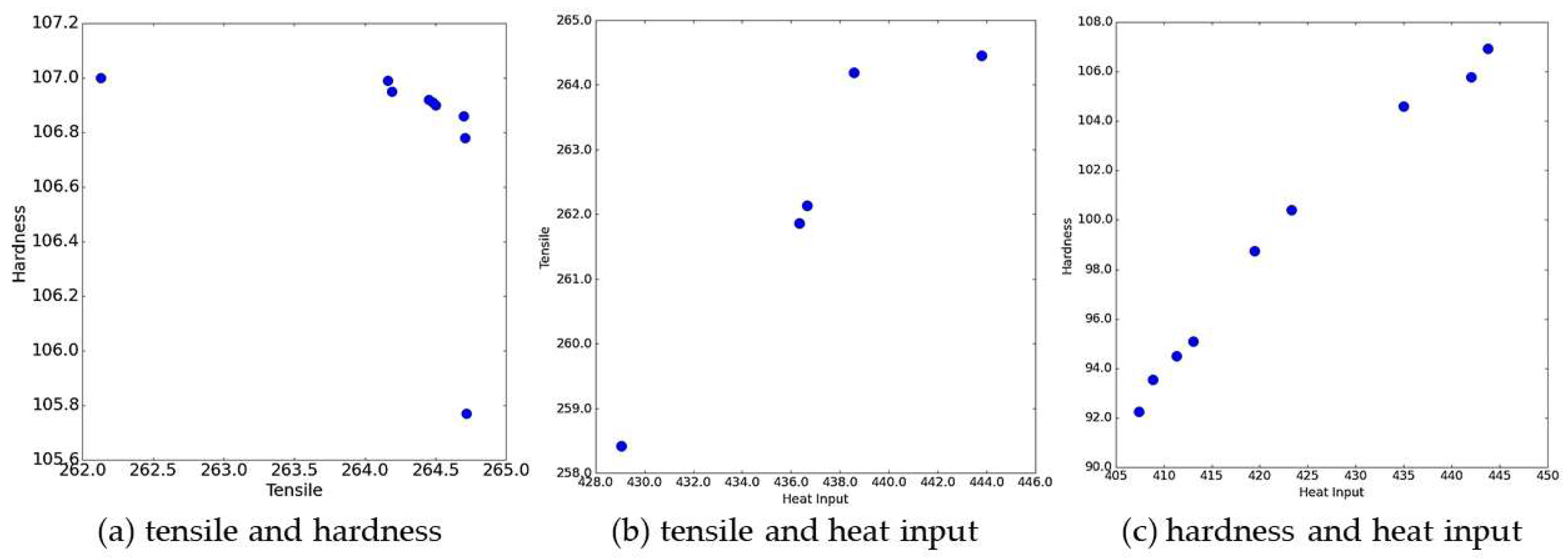
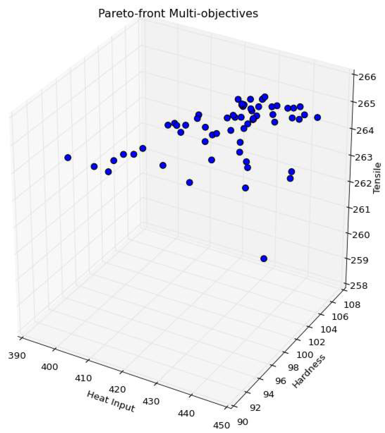
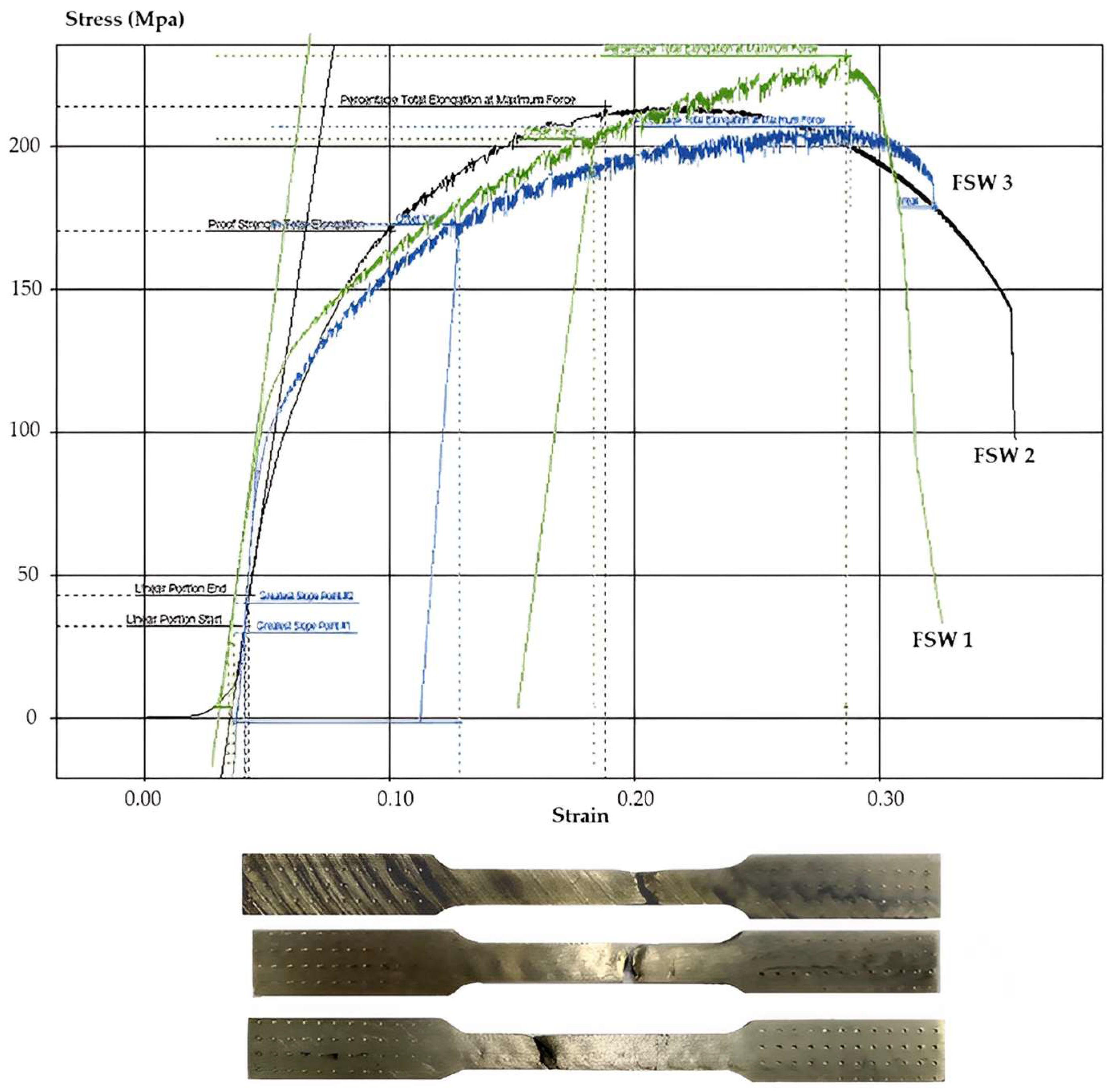
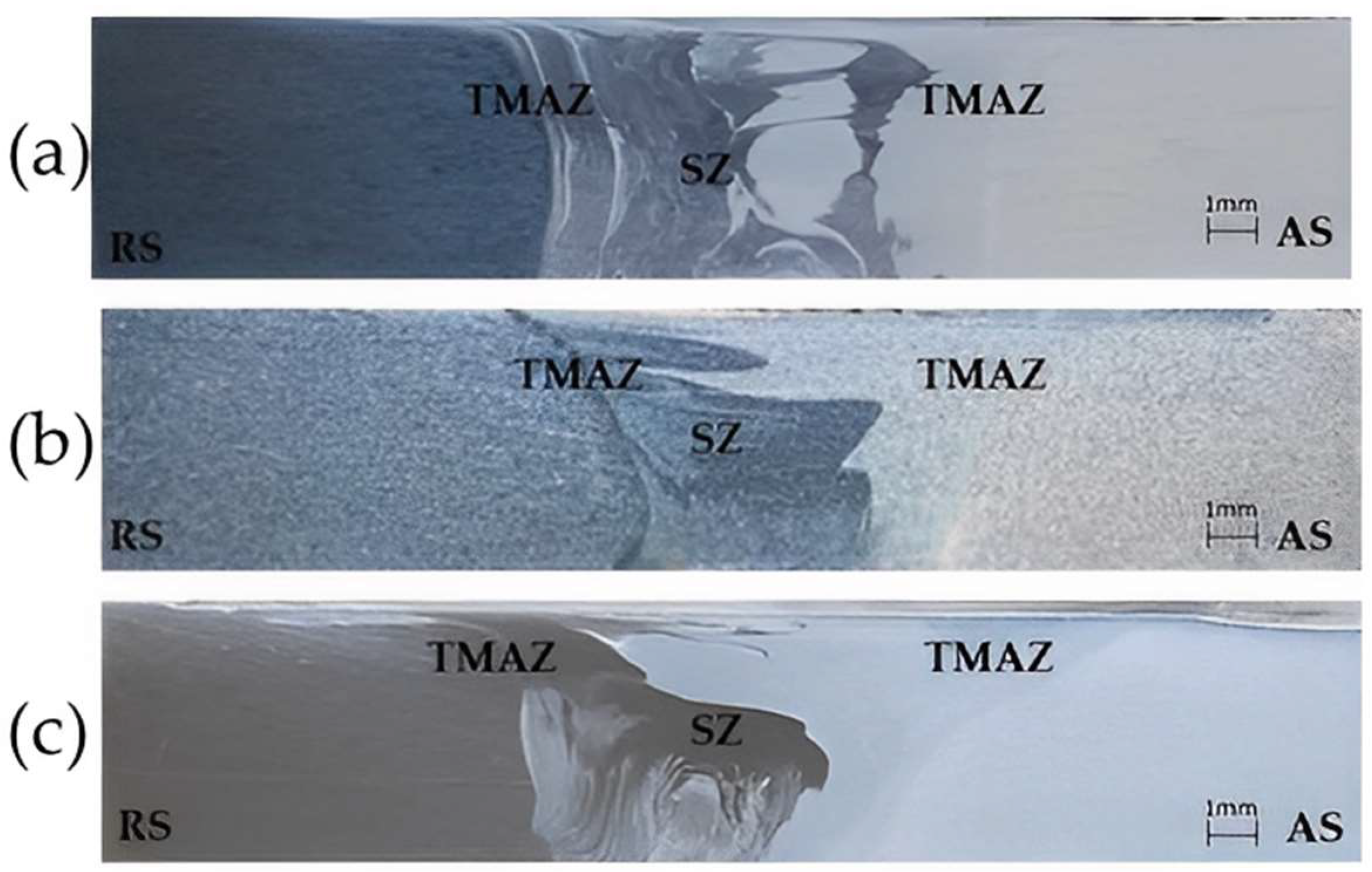
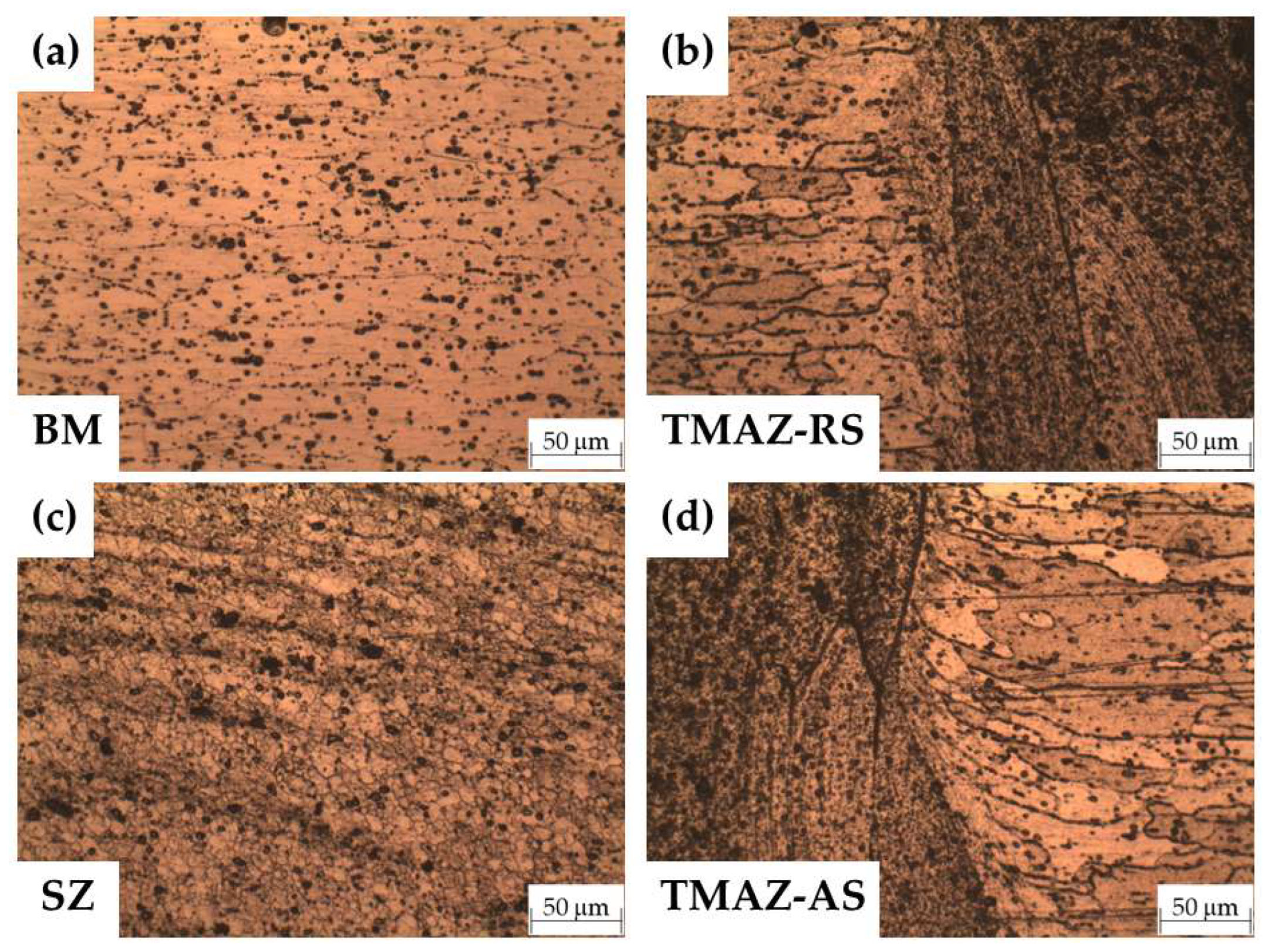
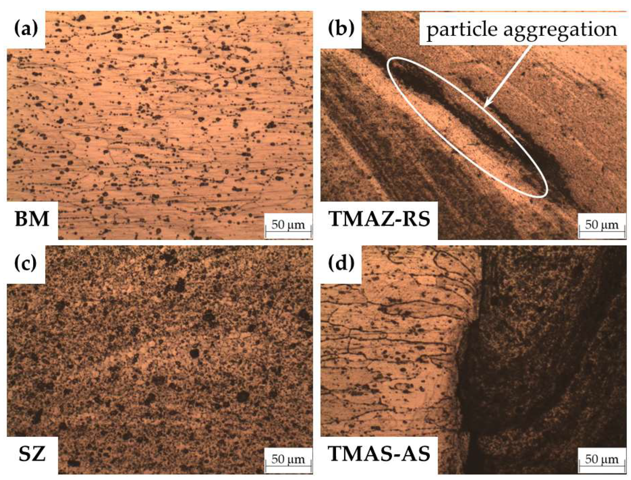
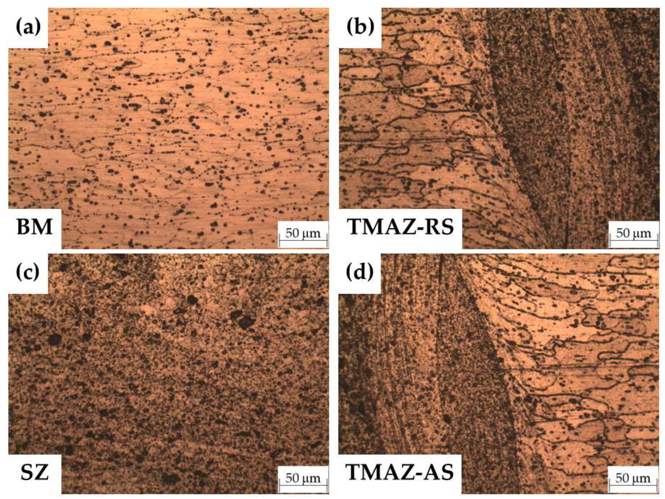
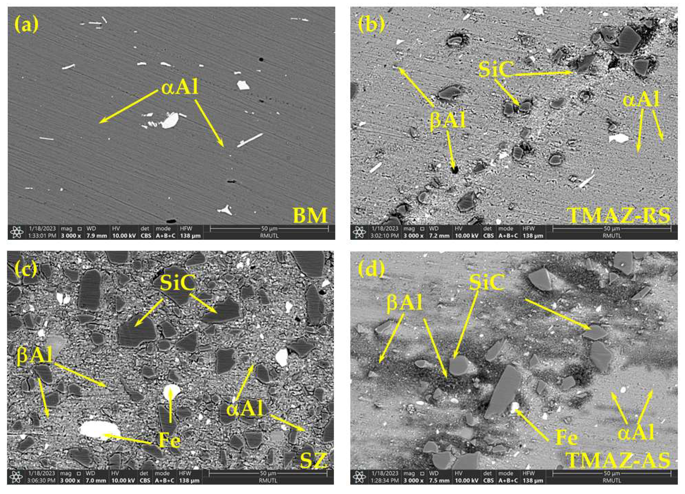
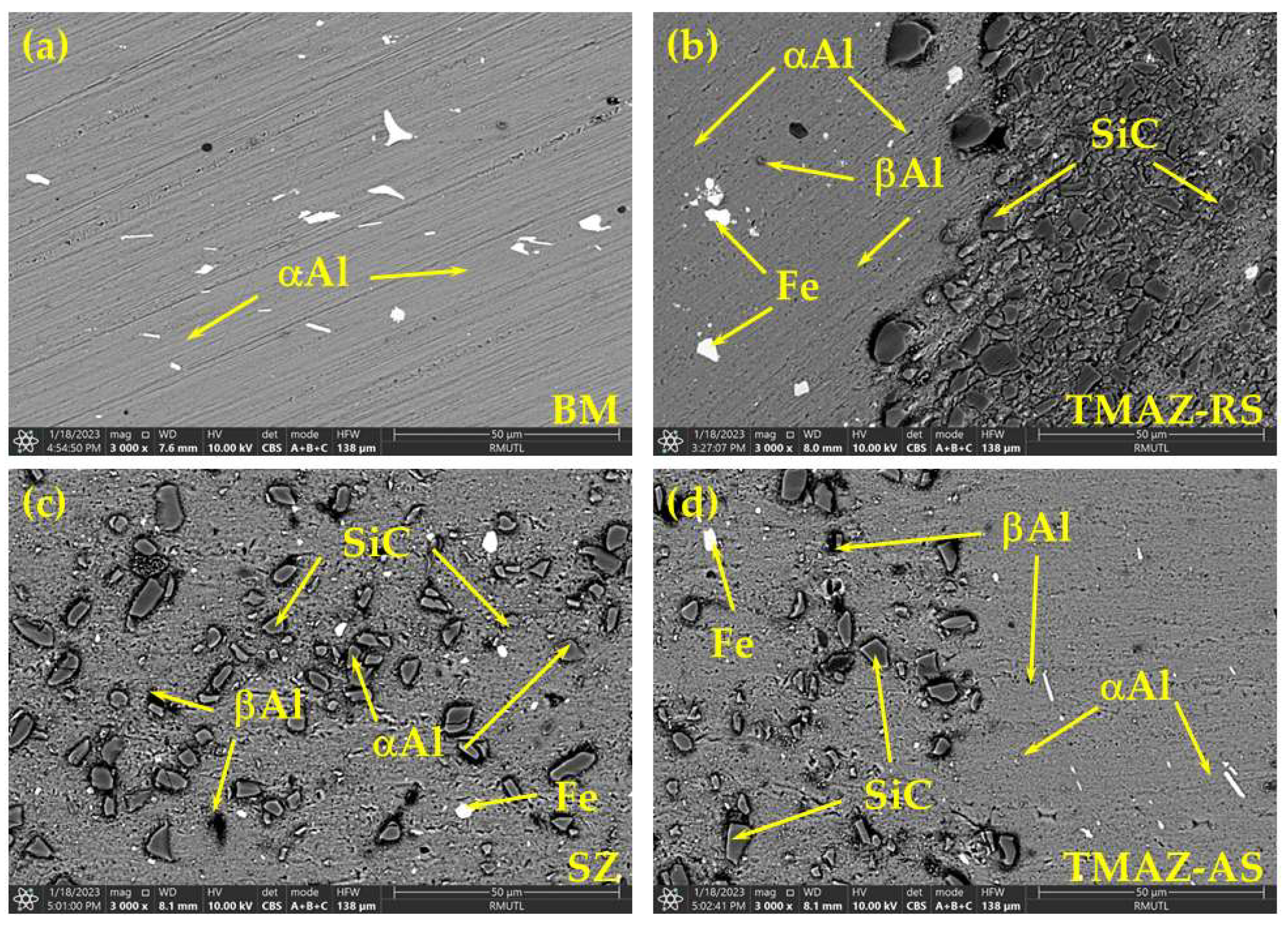
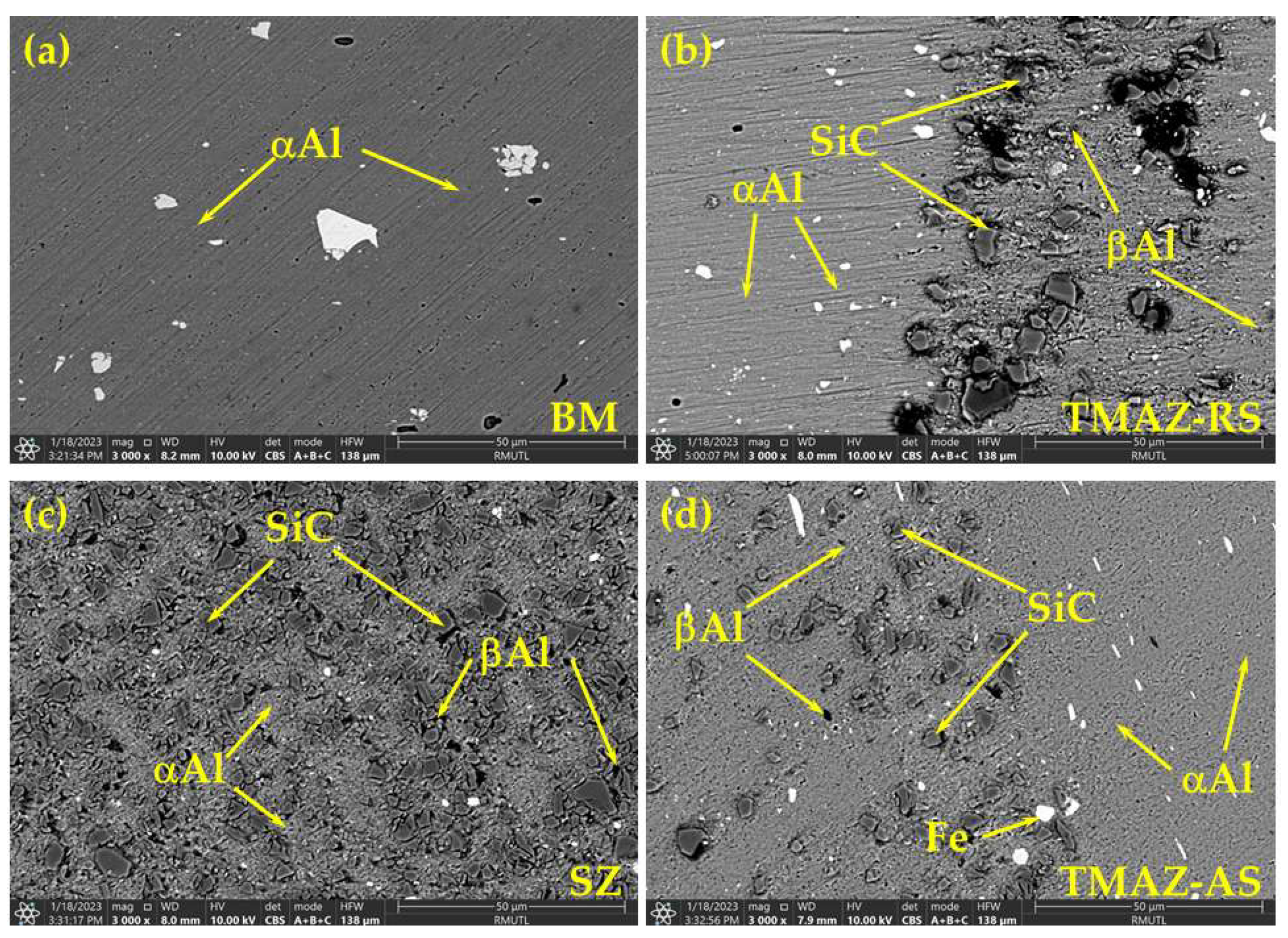
5. Microstructure Analysis

The experimental conditions used for the dissimilar welding process of AA5083 and AA6061 with particle reinforcement displayed different microstructures that affected the mechanical properties of the weld seam. The weld seam’s structure was determined by using microstructure photography. The microstructure of the weld seam between the optimal experimental and the confirmed experimental condition of the DE and MoDE was compared.

The characteristics observed in the weld seam’s structural investigation using the optical microscope were as follows: The optimal experimental conditions were RtS at 1500 rpm, WS at 15 mm/min, SD at 18.00 mm, TA at 3 degrees, a hexagon cylindrical pin type, SiC particle reinforcement, and straight tool pin movement direction, with a tensile strength of 246.32 MPa, hardness of 101.8 HV, and heat input of 443.5 °C in the welding process, respectively. The marcrostructure of the weld seam showed no defects or cracking in the SZ and TMAZ, as shown in Figure 12a. The area of SZ exhibited nonhomogenous of material and more material deformation in SZ and TMAZ. The weld seam microstructure of SZ displays the presence of small reinforcement particles but at a low number, as shown in Figure 13b–d. Due to the influence of the tool stirring on the sides of the RS and AS, there was a slight increase in the SiC reinforcement particles and the appearance of large and small reinforcement particles in the area of the TMAZ. When compared with the optimal welding condition of DE, it was found that the optimal welding condition of the original DE was an RtS of 993.67 rpm, WS of 76.63 mm/min, SD of 20.55 mm, and TA of 1.22 degrees, with a straight cylindrical pin, silicon carbide (SiC) reinforcement particles, and a straight tool pin movement direction that shows an optimal solution consisting of a UTS of 255.94 MPa, a hardness of 103.09 HV, and a heat input of 421.36 °C. The weld seam’s marcrostructure was free of flaws, cracks and more material mixing than optimal initial experiment condition show as Figure 12b. The microstructure in stir zone (SZ) displayed the presence of homogeneous materials, an increased number of reinforcement particles, and regular dispersion, as shown in Figure 14c. This led to increases in the UTS and MH. Notwithstanding, as shown in Figure 14b,d, the thermomechanical affect zone (TMAZ) exhibited the agglomeration of SiC particles in the retreating side (RS) but a low distribution of reinforcement particles and was non-homogeneous in the advancing side (AS) due to the decrease in rotation speeds and the tool tilt angle’s effect on the tool’s stirring effectiveness and material flow.

In the MoDE method, the optimal welding conditions were as follows: RtS: 1162.81 rpm; WS: 52.73 mm/min; SD: 21.17 mm; TA: 2.37 degrees; straight cylindrical pin; SiC reinforcement particles; straight tool pin movement direction. This produced an optimal solution of a UTS of 264.68 MPa, hardness of 105.56 HV, and heat input of 415.26 °C. When comparing the solution with the optimal solution obtained for the original DE and the optimal welding condition of the initial experiment, the optimal solution for the MoDE displayed good weld joint that is the best performance and affected the weld seam’s quality. By verifying the weld seam’s marcrostructure in SZ and TMAZ as show in Figure 12c, it was revealed that there were no defects or cracking, and good mixing of material in SZ. Moreover, the microstructure of material was homogeneous (Figure 15). The distribution of SiC reinforcement particles exhibited regularity and an increased number of SiC particles, which filled the area of SZ and TMAZ, as shown in Figure 15b–d, due to the presence of higher plastic deformations than in the optimal conditions of original DE and the optimal experiment.

The microstructure analysis conducted using SEM found that the optimal welding condition of the initial experiment showed no microdefects and microcracks in the weld seam. The microstructure appeared to be in the phases of α-Al and β-Al, with Fe particles and small SiC particles in the SZ and TMAZ-AS areas, as shown in Figure 16c,d. The wear of the stir tool in the welding process affected the Fe particles appearing in the structure. The TMAZ in the RS side area exhibited α-Al and β-Al phases, as shown in Figure 16b. Meanwhile, in the optimal condition, the original DE showed no microdefects but had high reinforcement particle agglomerations in the TMAZ area on two sides, as shown in Figure 17b,d. The SZ area displayed little dispersions of reinforcement particles but a higher distribution of reinforcement particles than in the optimal welding condition of the initial experiment. The microstructure exhibited a material base of α-Al and β-Al, a high number of Fe particles, and SiC particles in the SZ and TMAZ areas. The optimal condition of MoDE showed fewer Fe particles than in the optimal condition for DE and a good distribution of SiC particles in the SZ and TMAZ areas, which could be a mechanism for increasing the strength of the weld seam, as shown in Figure 18b–d. Moreover, the combination of materials in the SZ area was highly homogeneous. Therefore, the optimal condition of MoDE produced better mechanical properties than in the other optimal welding condition.

6. Discussion

In this study, we showed that the optimal parameters for the friction stir welding of dissimilar materials can be achieved via a four-step procedure. We utilized a D-optimal design to plan the experiment in order to determine the optimal outcome. This experiment incorporated seven input parameters and had three objectives. The multi-objective optimization model was developed with the aid of the Design-Expert software. From the experiment of Design-Expert design, experiment number 5 showed the following optimal experiment conditions: SD, TA, RtS, and WS values of 18 mm, 3 degrees, 1500 rpm, and 15 mm/min, respectively, and HC pin geometry, SiC as the reinforcement particles substance, and straight tool pin movement directions. This welding condition provides a high heat input that is sufficient for plastic deformations and facilitates the flow of materials and reinforcement particles from the retreating side to advancing side. In addition, a high tilt angle implicates increased turbulence flow, reinforcement particle distribution and good mixed material; HC pin geometries and straight tool pin movement provide a surface area and angularity that can impel the flow of materials effectively, as shown in. [88,89]. However, the high heat input in welding processes increases the grain’s recrystallization and grain growth [90], which can reduce the strengthening mechanism related with strain-hardening processes and the strength of the grain boundary in TMAZ and base material areas. Thus, the experimental result of the Design-Expert framework is not an optimal result and should be improved in order to increase the tensile strength and hardness. Design-Expert may be used to optimize the goal by addressing one objective at a time; it cannot optimize one objective while simultaneously taking another objective into account. The proposed methods can be utilized to solve a multi-objective model. A modified differential evolution algorithm is the methodology proposed here. These strategies are discussed for the first time in [23,24]. The computational results presented in [23,24] demonstrate that the suggested model outperformed the D-optimal design, genetic algorithm (GA), and differential evolution algorithm (DE) in terms of its results. The outcome of our model matches that of [23,24], indicating that the suggested model outperformed the existing techniques. Semi-solid material (SSM) ADC12 aluminum, which was subjected to symmetric FSW, was employed in [23]. In our investigation, materials AA6061-T6 and AA5083-H112 (asymmetric FSW) were utilized. This is the first model based on [23,24] used for discovering the optimal solution for the asymmetric friction stir welding processes of aluminum.

When optimizing a single objective value, it is possible to find a better solution than when optimizing all objectives simultaneously. In this study, we optimized each objective separately and discovered that the best UTS attained by optimizing a single objective was 264.68 MPa, which was 5.23% and 3.30% higher than when optimizing MH and HI, respectively. When optimizing UTS as opposed to MH, the maximum hardness of the weld seam was 1.33% lower. This effect transpires similarly when maximizing other single objectives. This implies that optimizing one target often diminishes the quality of other objectives when carried out correctly. The findings of reference [91] confirm this conclusion. The use of multiple objectives entails the compromises being made between many objectives. Using a single objective to improve each model yields a value that is inferior to the optimal objective value. However, there is no objective with a lower value than the optimal value of the single objective model, which differs by more than 4%. In contrast to single-objective optimization, the difference between objectives can be as high as 25%. Reference [23] provides support for this conclusion. Therefore, if one is interested in obtaining several responses, the multi-objective model and the method we provided would align with this aspect.

In this study, we created an algorithm for determining the optimal value of a multi-objective model. We utilized the same continuous input parameters as those used in Jia et al. (2022) [15], Kumar et al. (2021) [4], and Kumar et al. (2021) [7]. In these three studies, the other two parameters of importance were the tool’s manner of moving (straight line) and the employment of a straight pin type; these two parameters influenced and improved mechanical properties, defects, and joint ability according to [1,89,92]. The tensile strength and micro-hardness were utilized as the target responses. The yield strength (YS), ultimate tensile strength (UTS), and the elongation of the FSW were affected by controlled parameters, such as the rotational speed (RtS), welding speed (WS), and plunge depth, according to the findings of the existing body of research. The experiment was designed using the Taguchi method, which demonstrated the effect of the controlled factors on the expected response. Utilizing experiments, the optimal parameter was determined. In our research, we found a superior solution to the one discovered by the experiment by employing MoDE, which was an extension of the work of these researchers. Using a response weight of 80:10:10, we determined that the Lingo solution was 23.55% superior to the experimental result, which was in agreement with the findings of [24]. The MoDE method produced optimal welding conditions: RtS: 1162.81 rpm; WS: 52.73 mm/min; SD: 21.17 mm; TA: 2.37 degrees; straight cylindrical pin geometry; SiC reinforcement particles; straight tool pin movement direction. This method obtained the targeted response values—UTS of 264.68 MPa, hardness of 105.56 HV, and heat input of 415.26 °C—which comprise the optimal solution. The weld seam’s structure displays no defects or cracking, homogeneous materials, and regular reinforcement particles dispersion. This optimal welding condition could be suitable for controlling the heat input that will be appropriate for plastic deformations and promoting continuous material flow, as shown in [93]. Moreover, increased tool tilt angles produce high turbulence in materials in addition to welding movement, according to [94]. Therefore, the stirring motion of the tool can increase the flow of materials, material mixing processes, and the number of SiC reinforcement particles from the RS side to the AS side. Moreover, this heat input value displayed minor phenomena, such as gain recrystallization and grain growth, which comprise the strengthening mechanisms related to strain hardening and grain boundary strengthening processes in the SZ TMAZ and BM areas, as shown in [95,96]. The weld seam’s structure exhibited three good strengthening mechanisms—particles reinforcement strengthening, strain hardening and grain boundary strengthening—which produce superior tensile strength and hardness when compared with different welding conditions.

Rani et al. (2022) [18], Moradi et al. (2019) [20], Moradi et al. (2017) [29], and Tabasi et al. (2016) [19] proposed that the use of SiC as the reinforcement particle influences the UTS of the welded output. These studies conclude that the addition of the reinforcement particles to the weld seam alters the mechanical properties of the welding seam, thus confirming the findings of earlier studies. In addition, in this study, we examined three mechanical welding property responses to determine which objectives out of UTS, MH, and HI have the greatest influence on the reinforcement particle of SiC and aluminum oxide. We discovered that hardness (MH) is the most important parameter because adding SiC to the system increases the hardness by 2.41% compared to adding aluminum oxide to the welding process, although the differences between UTS and HI when using different reinforcement particles are 11.49% and 6.24%, respectively. This conclusion corresponds with that of previous studies [66,97], which confirm that the addition of different types of reinforcement particles might impact the mechanical properties and other aspects of the weld seam differently.

7. Conclusions

In this investigation, we found the optimal FSW parameters based on three parameters: ultimate tensile strength (UTS), maximum hardness (MH), and minimum heat input (HI). Optimal parameter and objective values can be determined by using a four-step method. These steps involve the following: (1) performing experiments with seven controlled parameters to optimize three objectives using a D-optimal design; (2) constructing a multi-objective mathematical model using the Design-Expert software; (3) developing a modified differential evolution algorithm to solve the multi-objective model; and (4) applying the result obtained from (3) to the experiment to verify the value of the parameters and objectives. Friction stir welding was employed to join dissimilar aluminum alloys, AA6061 and AA5083, by utilizing the proposed approach. The following bullet points summarize the key findings of this study:

(1)

This study reveals, for the first time, the best welding conditions for AA6061 and AA5083. Seven parameters simultaneously subjected to three objectives have been explored.

(2)

The modified differential evolution algorithm is the method that has been devised to locate the optimal parameters of the FSW (MoDE). Using Pareto front and TOPSIS, the optimal parameter among several types of comparative approaches has been analyzed. The methods that were compared for MoDE include the initial DE and PSO.

(3)

Using MoDE, Pareto front analysis, and TOPIS, the following is the best set of parameters: (1) rotational speed of 1162.81 rpm, (2) welding speed of 52.73 mm/min, (3) shoulder diameter of 21.17 mm, (4) tilt angle of 2.37 degrees, (5) pin-type straight cylindrical, (6) silicon carbide reinforcement particles, and (7) straight tool pin movement direction. The optimal responses (objective) of the asymmetric FSW are as follows. The material has (1) an ultimate tensile strength of 264.68 MPa, (2) a maximum hardness of 105.56 HV, and (3) a maximum heat input of 415.26 °C.

(4)

MODE has been implemented and compared to three methods: (1) a genuine experiment utilizing D-optimal design, (2) particle swarm optimization (PSO), and (3) the original DE. The computational results demonstrated that MoDE provides a superior solution to the experiment, PSO, and the original DE by 7.45%, 4.45%, and 3.5%, respectively. The proposed methods provide superior UTS, MH, and HI than other methods by an average of 8.04%, 4.44%, and 2.44%, respectively.

(5)

The reliability of the optimal parameters from the theory acquired from different methods has been checked by completing 30 actual experiments for each method. The computational result of the result verification model revealed that PSO, original DE, and MODE produce experimental and theoretical value differences of 5.19%, 3.71%, and 1.49%, respectively. This indicates that MoDE has the highest level of reliability compared to the other approaches.

Future research subjects that can be expanded upon by using the fundamental concept of our study can be classified into three categories. The controlled parameter perspective is the first intriguing area. The literature review revealed that other characteristics—such as tool pin movement directions, penetration, and methods for adding reinforcement particles—have been explored in FSW research; consequently, these parameters can be incorporated into the suggested model. In addition to UTS, MH, and HI, researchers are interested in additional objectives or responses, such as the bending and elongation phenomena of the weld seam. This can also be incorporated into the model in order to simultaneously confirm the optimal value for all objectives. Finally, a more efficient method can be designed to replace MoDE in order to enhance the quality of the result. Currently, the available new methods include artificial and multiple intelligence, variable neighborhood strategy adaptive search, and hybrid variants of various methods.

References

1. Verma, S.; Kumar, V. Optimization of friction stir welding parameters of dissimilar aluminium alloys 6061 and 5083 by using response surface methodology. Proc. Inst. Mech. Eng. Part C J. Mech. Eng. Sci. 2021, 235, 7009–7020. [Google Scholar] [CrossRef]
2. Ramesh, N.; Kumar, V.S. Experimental erosion-corrosion analysis of friction stir welding of AA 5083 and AA 6061 for sub-sea applications. Appl. Ocean Res. 2020, 98, 102121. [Google Scholar] [CrossRef]
3. Selamat, N.; Baghdadi, A.; Sajuri, Z.; Junaidi, S.; Kokabi, A. Rolling effect on dissimilar friction stir welded AA5083-AA6061 aluminium alloy joints. J. Adv. Manuf. Technol. 2020, 14, 49–61. [Google Scholar]
4. Kumar, K.K.; Kumar, A.; Satyanarayana, M. Enhancing corrosion resistance and mechanical properties of dissimilar friction stir welded 5083-6061 aluminium alloys using external cooling environment. Proc. Inst. Mech. Eng. Part L J. Mater. Des. Appl. 2021, 235, 2692–2708. [Google Scholar] [CrossRef]
5. Saravanakumar, R.; Rajasekaran, T.; Pandey, C. Optimisation of underwater friction stir welding parameters of aluminum alloy AA5083 using RSM and GRA. Proc. Inst. Mech. Eng. Part E J. Process Mech. Eng. 2022, 09544089221134446. [Google Scholar] [CrossRef]
6. Saravanakumar, R.; Rajasekaran, T.; Pandey, C.; Menaka, M. Mechanical and Microstructural Characteristics of Underwater Friction Stir Welded AA5083 Armor-Grade Aluminum Alloy Joints. J. Mater. Eng. Perform. 2022, 31, 8459–8472. [Google Scholar] [CrossRef]
7. Kumar, K.K.; Kumar, A.; Satyanarayana, M. Effect of friction stir welding parameters on the material flow, mechanical properties and corrosion behavior of dissimilar AA5083-AA6061 joints. Proc. Inst. Mech. Eng. Part C J. Mech. Eng. Sci. 2022, 236, 2901–2917. [Google Scholar] [CrossRef]
8. Chen, S.; Zhang, H.; Jiang, X.; Yuan, T.; Han, Y.; Li, X. Mechanical properties of electric assisted friction stir welded 2219 aluminum alloy. J. Manuf. Process. 2019, 44, 197–206. [Google Scholar] [CrossRef]
9. Meng, X.; Huang, Y.; Cao, J.; Shen, J.; dos Santos, J.F. Recent progress on control strategies for inherent issues in friction stir welding. Prog. Mater. Sci. 2021, 115, 100706. [Google Scholar] [CrossRef]
10. Elatharasan, G.; Manikandan, R.; Karthikeyan, G. Multi-response optimization of process parameters in friction stir welding of dissimilar aluminum alloys by Grey relation analysis (AA 6061-T6 & AA5083-H111). Mater. Today Proc. 2021, 37, 1172–1182. [Google Scholar] [CrossRef]
11. Rao, D.; Huber, K.; Heerens, J.; dos Santos, J.; Huber, N. Asymmetric mechanical properties and tensile behaviour prediction of aluminium alloy 5083 friction stir welding joints. Mater. Sci. Eng. A 2013, 565, 44–50. [Google Scholar] [CrossRef]
12. Ji, H.; Deng, Y.; Xu, H.; Lin, S.; Wang, W.; Dong, H. The mechanism of rotational and non-rotational shoulder affecting the microstructure and mechanical properties of Al-Mg-Si alloy friction stir welded joint. Mater. Des. 2020, 192, 108729. [Google Scholar] [CrossRef]
13. Chennaiah, M.B.; Kumar, K.R.; Sridhar, V. Influence of tool profiles on similar Al-5083 alloys using friction stir welding. Mater. Today Proc. 2021, 46, 8032–8037. [Google Scholar] [CrossRef]
14. Xu, W.; Lu, H.; Li, X.; Wang, M.; Ma, J.; Luo, Y. Microstructure evolution and stress corrosion cracking sensitivity of friction stir welded high strength AA7085 joint. Mater. Des. 2021, 212, 110297. [Google Scholar] [CrossRef]
15. Jia, H.; Wu, K.; Sun, Y.; Hu, F.; Chen, G. Evaluation of axial force, tool torque and weld quality of friction stir welded dissimilar 6061/5083 aluminum alloys. CIRP J. Manuf. Sci. Technol. 2022, 37, 267–277. [Google Scholar] [CrossRef]
16. Sidhom, A.A.; Naga, S.A.; Kamal, A. Friction stir spot welding of similar and dissimilar high density polyethylene and polypropylene sheets. Adv. Ind. Manuf. Eng. 2022, 4, 100076. [Google Scholar] [CrossRef]
17. MirHashemi, S.; Amadeh, A.; Khodabakhshi, F. Effects of SiC nanoparticles on the dissimilar friction stir weldability of low-density polyethylene (LDPE) and AA7075 aluminum alloy. J. Mater. Res. Technol. 2021, 13, 449–462. [Google Scholar] [CrossRef]
18. Rani, P.; Mishra, R. Influence of Reinforcement with Multi-Pass FSW on the Mechanical and Microstructural Behavior of Dissimilar Weld Joint of AA5083 and AA6061. Silicon 2022, 14, 11219–11233. [Google Scholar] [CrossRef]
19. Tabasi, M.; Farahani, M.; Givi, M.K.B.; Farzami, M.R.; Moharami, A. Dissimilar friction stir welding of 7075 aluminum alloy to AZ31 magnesium alloy using SiC nanoparticles. Int. J. Adv. Manuf. Technol. 2016, 86, 705–715. [Google Scholar] [CrossRef]
20. Moradi, M.M.; Aval, H.J.; Jamaati, R.; Amirkhanlou, S.; Ji, S. Effect of SiC nanoparticles on the microstructure and texture of friction stir welded AA2024/AA6061. Mater. Charact. 2019, 152, 169–179. [Google Scholar] [CrossRef]
21. Kumar, H.A.; Ramana, V.V. Influence of tool parameters on the tensile properties of friction stir welded aluminium 5083 and 6082 alloys. Mater. Today Proc. 2020, 27, 951–957. [Google Scholar] [CrossRef]
22. Padhy, G.; Wu, C.; Gao, S. Friction stir based welding and processing technologies-processes, parameters, microstructures and applications: A review. J. Mater. Sci. Technol. 2018, 34, 1–38. [Google Scholar] [CrossRef]
23. Chainarong, S.; Pitakaso, R.; Sirirak, W.; Srichok, T.; Khonjun, S.; Sethanan, K.; Sangthean, T. Multi-Objective Variable Neighborhood Strategy Adaptive Search for Tuning Optimal Parameters of SSM-ADC12 Aluminum Friction Stir Welding. J. Manuf. Mater. Process. 2021, 5, 123. [Google Scholar] [CrossRef]
24. Chainarong, S.; Srichok, T.; Pitakaso, R.; Sirirak, W.; Khonjun, S.; Akararungruangku, R. Variable Neighborhood Strategy Adaptive Search for Optimal Parameters of SSM-ADC 12 Aluminum Friction Stir Welding. Processes 2021, 9, 1805. [Google Scholar] [CrossRef]
25. Fuse, K.; Badheka, V.; Patel, V.; Andersson, J. Dual sided composite formation in Al 6061/B4C using novel bobbin tool friction stir processing. J. Mater. Res. Technol. 2021, 13, 1709–1721. [Google Scholar] [CrossRef]
26. Kianezhad, M.; Raouf, A.H. Effect of nano-Al2O3 particles and friction stir processing on 5083 TIG welding properties. J. Mater. Process. Technol. 2019, 263, 356–365. [Google Scholar] [CrossRef]
27. Bodaghi, M.; Dehghani, K. Friction stir welding of AA5052: The effects of SiC nano-particles addition. Int. J. Adv. Manuf. Technol. 2017, 88, 2651–2660. [Google Scholar] [CrossRef]
28. Karthikeyan, P.; Mahadevan, K. Investigation on the effects of SiC particle addition in the weld zone during friction stir welding of Al 6351 alloy. Int. J. Adv. Manuf. Technol. 2015, 80, 1919–1926. [Google Scholar] [CrossRef]
29. Moradi, M.M.; Aval, H.J.; Jamaati, R. Effect of pre and post welding heat treatment in SiC-fortified dissimilar AA6061-AA2024 FSW butt joint. J. Manuf. Process. 2017, 30, 97–105. [Google Scholar] [CrossRef]
30. Zhang, H.; Luo, S.; Xu, W. Influence of Welding Speed on Zigzag Line Feature and Tensile Property of a Friction-Stir-Welded Al-Zn-Mg Aluminum Alloy. J. Mater. Eng. Perform. 2019, 28, 1790–1800. [Google Scholar] [CrossRef]
31. Cabibbo, M.; Forcellese, A.; Santecchia, E.; Paoletti, C.; Spigarelli, S.; Simoncini, M. New Approaches to Friction Stir Welding of Aluminum Light-Alloys. Metals 2020, 10, 233. [Google Scholar] [CrossRef]
32. Sharma, N.; Khan, Z.A.; Siddiquee, A.N.; Wahid, M.A. Multi-response optimization of friction stir welding process parameters for dissimilar joining of Al6101 to pure copper using standard deviation based TOPSIS method. Proc. Inst. Mech. Eng. Part C J. Mech. Eng. Sci. 2019, 233, 6473–6482. [Google Scholar] [CrossRef]
33. Wakchaure, K.; Thakur, A.; Gadakh, V.; Kumar, A. Multi-Objective Optimization of Friction Stir Welding of Aluminium Alloy 6082-T6 Using hybrid Taguchi-Grey Relation Analysis- ANN Method. Mater. Today Proc. 2018, 5, 7150–7159. [Google Scholar] [CrossRef]
34. Kamal Babu, K.; Panneerselvam, K.; Sathiya, P.; Noorul Haq, A.; Sundarrajan, S.; Mastanaiah, P.; Srinivasa Murthy, C. Parameter optimization of friction stir welding of cryorolled AA2219 alloy using artificial neural network modeling with genetic algorithm. Int. J. Adv. Manuf. Technol. 2018, 94, 3117–3129. [Google Scholar] [CrossRef]
35. Tamjidy, M.; Baharudin, B.T.H.T.; Paslar, S.; Matori, K.A.; Sulaiman, S.; Fadaeifard, F. Multi-Objective Optimization of Friction Stir Welding Process Parameters of AA6061-T6 and AA7075-T6 Using a Biogeography Based Optimization Algorithm. Materials 2017, 10, 533. [Google Scholar] [CrossRef] [PubMed] [Green Version]
36. Gupta, S.K.; Pandey, K.; Kumar, R. Multi-objective optimization of friction stir welding process parameters for joining of dissimilar AA5083/AA6063 aluminum alloys using hybrid approach. Proc. Inst. Mech. Eng. Part L J. Mater. Des. Appl. 2018, 232, 343–353. [Google Scholar] [CrossRef]
37. Kesharwani, R.; Panda, S.; Pal, S. Multi Objective Optimization of Friction Stir Welding Parameters for Joining of Two Dissimilar Thin Aluminum Sheets. Procedia Mater. Sci. 2014, 6, 178–187. [Google Scholar] [CrossRef] [Green Version]
38. Senthil, S.M.; Parameshwaran, R.; Nathan, S.R.; Kumar, M.B.; Deepandurai, K. A multi-objective optimization of the friction stir welding process using RSM-based-desirability function approach for joining aluminum alloy 6063-T6 pipes. Struct. Multidiscip. Optim. 2020, 62, 1117–1133. [Google Scholar] [CrossRef]
39. Goyal, A.; Garg, R.K. Parametric optimization of friction stir welding process for marine grade aluminum alloy. Int. J. Struct. Integr. 2019, 10, 162–175. [Google Scholar] [CrossRef]
40. Roshan, S.B.; Jooibari, M.B.; Teimouri, R.; Asgharzadeh-Ahmadi, G.; Falahati-Naghibi, M.; Sohrabpoor, H. Optimization of friction stir welding process of AA7075 aluminum alloy to achieve desirable mechanical properties using ANFIS models and simulated annealing algorithm. Int. J. Adv. Manuf. Technol. 2013, 69, 1803–1818. [Google Scholar] [CrossRef]
41. Srichok, T.; Pitakaso, R.; Sethanan, K.; Sirirak, W.; Kwangmuang, P. Combined response surface method and modified differential evolution for parameter optimization of friction stir welding. Processes 2020, 8, 1080. [Google Scholar] [CrossRef]
42. Chokanat, P.; Pitakaso, R.; Sethanan, K. Methodology to Solve a Special Case of the Vehicle Routing Problem: A Case Study in the Raw Milk Transportation System. AgriEngineering 2019, 1, 75–93. [Google Scholar] [CrossRef] [Green Version]
43. Pijitbanjong, P.; Akararungruangkul, R.; Pitakaso, R.; Sethanan, K. Improved differential evolution algorithms for solving multi-stage crop planning model in southern region of Thailand. Songklanakarin J. Sci. Technol. 2019, 41, 1116–1123. [Google Scholar]
44. Maniscalco, J.; Elmustafa, A.A.; Bhukya, S.; Wu, Z. Numerical Simulation of the Donor-Assisted Stir Material for Friction Stir Welding of Aluminum Alloys and Carbon Steel. Metals 2023, 13, 164. [Google Scholar] [CrossRef]
45. Khan, M.; Rehman, A.; Aziz, T.; Shahzad, M.; Naveed, K.; Subhani, T. Effect of inter-cavity spacing in friction stir processed Al 5083 composites containing carbon nanotubes and boron carbide particles. J. Mater. Process. Technol. 2018, 253, 72–85. [Google Scholar] [CrossRef]
46. Prabha, K.A.; Putha, P.K.; Prasad, B.S. Effect of Tool Rotational Speed on Mechanical Properties of Aluminium Alloy 5083 Weldments in Friction Stir Welding. Mater. Today Proc. 2018, 5, 18535–18543. [Google Scholar] [CrossRef]
47. Kumar, P.S.; Devaraju, A. Influence of Tool Rotational speed and Pin Profile on Mechanical and Microstructural Characterization of Friction Stir Welded 5083 Aluminium Alloy. Mater. Today Proc. 2018, 5, 3518–3523. [Google Scholar] [CrossRef]
48. Tayebi, P.; Fazli, A.; Asadi, P.; Soltanpour, M. Formability analysis of dissimilar friction stir welded AA 6061 and AA 5083 blanks by SPIF process. CIRP J. Manuf. Sci. Technol. 2019, 25, 50–68. [Google Scholar] [CrossRef]
49. Ma, X.; Xu, S.; Wang, F.; Zhao, Y.; Meng, X.; Xie, Y.; Wan, L.; Huang, Y. Effect of Temperature and Material Flow Gradients on Mechanical Performances of Friction Stir Welded AA6082-T6 Joints. Materials 2022, 15, 6579. [Google Scholar] [CrossRef]
50. Rodriguez, R.; Jordon, J.; Allison, P.; Rushing, T.; Garcia, L. Microstructure and mechanical properties of dissimilar friction stir welding of 6061-to-7050 aluminum alloys. Mater. Des. 2015, 83, 60–65. [Google Scholar] [CrossRef]
51. Azeez, S.; Mashinini, M.; Akinlabi, E. Sustainability of friction stir welded AA6082 plates through post-weld solution heat treatment. Procedia Manuf. 2019, 33, 27–34. [Google Scholar] [CrossRef]
52. Kalinenko, A.; Vysotskii, I.; Malopheyev, S.; Mironov, S.; Kaibyshev, R. Relationship between welding conditions, abnormal grain growth and mechanical performance in friction-stir welded 6061-T6 aluminum alloy. Mater. Sci. Eng. A 2021, 817, 141409. [Google Scholar] [CrossRef]
53. Fu, H.; Chai, Z.; Han, S.; Liu, D.; Chang, Y.; Chen, Y.; Li, Y.; Zhang, J.; Xu, Y.; Zhang, K.; et al. Effect of post-weld heat treatment on a friction stir welded joint between 9Cr-ODS and CLF-1 steels. Mater. Charact. 2022, 187, 111868. [Google Scholar] [CrossRef]
54. Mohamed, J.U.; Palaniappan, P.K.; Maran, P. Influence of post weld heat treatment on the tensile and microhardness characteristics of friction stir welded joints of AA6082/ZrO2/B4C composites. Mater. Today Proc. 2022, 56, 902–909. [Google Scholar] [CrossRef]
55. Sathish, T.; Kaladgi, A.R.R.; Mohanavel, V.; Arul, K.; Afzal, A.; Aabid, A.; Baig, M.; Saleh, B. Experimental Investigation of the Friction Stir Weldability of AA8006 with Zirconia Particle Reinforcement and Optimized Process Parameters. Materials 2021, 14, 2782. [Google Scholar] [CrossRef]
56. Ali, K.S.A.; Mohanavel, V.; Vendan, S.A.; Ravichandran, M.; Yadav, A.; Gucwa, M.; Winczek, J. Mechanical and microstructural characterization of friction stir welded SiC and B4C reinforced aluminium alloy AA6061 metal matrix composites. Materials 2021, 14, 3110. [Google Scholar] [CrossRef]
57. Sadeghi, B.; Sadeghian, B.; Taherizadeh, A.; Laska, A.; Cavaliere, P.; Gopinathan, A. Effect of Porosity on the Thermo-Mechanical Behavior of Friction-Stir-Welded Spark-Plasma-Sintered Aluminum Matrix Composites with Bimodal Micro-and Nano-Sized Reinforcing Al2O3 Particles. Metals 2022, 12, 1660. [Google Scholar] [CrossRef]
58. Zubcak, M.; Soltes, J.; Zimina, M.; Weinberger, T.; Enzinger, N. Investigation of Al-B4C Metal Matrix Composites Produced by Friction Stir Additive Processing. Metals 2021, 11, 2020. [Google Scholar] [CrossRef]
59. Tan, Z.; Li, J.; Zhang, Z. Experimental and numerical studies on fabrication of nanoparticle reinforced aluminum matrix composites by friction stir additive manufacturing. J. Mater. Res. Technol. 2021, 12, 1898–1912. [Google Scholar] [CrossRef]
60. Señorís-Puentes, S.; Serrano, R.F.; González-Doncel, G.; Hattel, J.H.; Mishin, O.V. Microstructure and Mechanical Properties of Friction Stir Welded AA6061/AA6061 + 40 vol% SiC Plates. Metals 2021, 11, 206. [Google Scholar] [CrossRef]
61. Chaudhary, N.; Singh, S.; Garg, M.P.; Garg, H.K.; Sharma, S.; Li, C.; Eldin, E.M.T.; El-Khatib, S. Parametric Optimisation of Friction-Stir-Spot-Welded Al 6061-T6 Incorporated with Silicon Carbide Using a Hybrid WASPAS–Taguchi Technique. Materials 2022, 15, 6427. [Google Scholar] [CrossRef] [PubMed]
62. Ostovan, F.; Hasanzadeh, E.; Toozandehjani, M.; Shafiei, E.; Jamaludin, K.R.; Amrin, A.B. A combined friction stir processing and ball milling route for fabrication Al5083-Al2O3 nanocomposite. Mater. Res. Express 2019, 6, 065012. [Google Scholar] [CrossRef]
63. Sharma, A.; Sharma, V.M.; Paul, J. A comparative study on microstructural evolution and surface properties of graphene/CNT reinforced Al6061−SiC hybrid surface composite fabricated via friction stir processing. Trans. Nonferrous Met. Soc. China 2019, 29, 2005–2026. [Google Scholar] [CrossRef]
64. Parumandla, N.; Adepu, K. Effect of tool shoulder geometry on fabrication of Al/Al2O3 surface nano composite by friction stir processing. Part. Sci. Technol. 2020, 38, 121–130. [Google Scholar] [CrossRef]
65. Yu, X.; Wu, H.; Guo, L.; Duan, L.; Xiu, W. Investigating on microstructural and mechanical properties of Al6061/nano–SiC composites fabricated via friction stir processing. Mater. Res. Express 2020, 7, 026554. [Google Scholar] [CrossRef]
66. Moosavi, S.E.; Movahedi, M.; Kazeminezhad, M. Friction stir welding of severely plastic deformed aluminum using (Al2O3 + graphite) hybrid powders: Grain structure stability and mechanical performance. J. Mater. Res. Technol. 2022, 21, 961–980. [Google Scholar] [CrossRef]
67. Palanivel, S.; Nelaturu, P.; Glass, B.; Mishra, R. Friction stir additive manufacturing for high structural performance through microstructural control in an Mg based WE43 alloy. Mater. Des. 2015, 65, 934–952. [Google Scholar] [CrossRef]
68. Jia, H.; Wu, K.; Sun, Y. Numerical and experimental study on the thermal process, material flow and welding defects during high-speed friction stir welding. Mater. Today Commun. 2022, 31, 103526. [Google Scholar] [CrossRef]
69. Campanella, D.; Marcon, G.; Lombardo, A.; Buffa, G.; Fratini, L. The role of thermal contribution in the design of AA2024 friction stir welded butt and lap joints: Mechanical properties and energy demand. Prod. Eng. 2022, 16, 247–259. [Google Scholar] [CrossRef]
70. Ni, Y.; Liu, Y.; Zhang, P.; Huang, J.; Yu, X. Thermal cycles, microstructures and mechanical properties of AA7075-T6 ultrathin sheet joints produced by high speed friction stir welding. Mater. Charact. 2022, 187, 111873. [Google Scholar] [CrossRef]
71. Surya Sinivas Raju, D.; Vaira Vignesh, R.; Padmanaban, R. Computational Modeling of Thermal Phenomenon in Friction Stir Welding of ASTM A710 Steel with AA5083 Alloy. In Recent Advances in Energy Technologies; Springer Nature: Singapore, 2022; pp. 629–640. [Google Scholar] [CrossRef]
72. Leon, J.S.; Franklin, V.A.; Ravi, R.; Geetha, B. Numerical thermal modeling on tool and backing plate diffusivity in friction stir welding using non-circular tool pin. Mater. Today Proc. 2022, 51, 374–380. [Google Scholar] [CrossRef]
73. Janeczek, A.; Tomków, J.; Fydrych, D. The Influence of Tool Shape and Process Parameters on the Mechanical Properties of AW-3004 Aluminium Alloy Friction Stir Welded Joints. Materials 2021, 14, 3244. [Google Scholar] [CrossRef] [PubMed]
74. Ghiasvand, A.; Yavari, M.M.; Tomków, J.; Grimaldo Guerrero, J.W.; Kheradmandan, H.; Dorofeev, A.; Memon, S.; Derazkola, H.A. Investigation of Mechanical and Microstructural Properties of Welded Specimens of AA6061-T6 Alloy with Friction Stir Welding and Parallel-Friction Stir Welding Methods. Materials 2021, 14, 6003. [Google Scholar] [CrossRef] [PubMed]
75. Bossle, E.P.; Vicharapu, B.; Lemos, G.V.B.; Lessa, C.R.D.L.; Bergmann, L.; dos Santos, J.F.; Clarke, T.G.R.; De, A. Friction Stir Lap Welding of Inconel 625 and a High Strength Steel. Metals 2023, 13, 146. [Google Scholar] [CrossRef]
76. Khedr, M.; Hamada, A.; Järvenpää, A.; Elkatatny, S.; Abd-Elaziem, W. Review on the Solid-State Welding of Steels: Diffusion Bonding and Friction Stir Welding Processes. Metals 2022, 13, 54. [Google Scholar] [CrossRef]
77. Yuan, B.; Liao, D.; Jiang, W.; Deng, H.; Li, G. Study on Friction and Wear Properties and Mechanism at Different Temperatures of Friction Stir Lap Welding Joint of SiCp/ZL101 and ZL101. Metals 2022, 13, 3. [Google Scholar] [CrossRef]
78. Khalafe, W.H.; Sheng, E.L.; Bin Isa, M.R.; Omran, A.B.; Bin Shamsudin, S. The Effect of Friction Stir Welding Parameters on the Weldability of Aluminum Alloys with Similar and Dissimilar Metals. Metals 2022, 12, 2099. [Google Scholar] [CrossRef]
79. Miao, H.; Miura, T.; Jiang, W.; Okada, M.; Otsu, M. Effect of Shoulder Fillet Radius on Welds in Bobbin Tool Friction Stir Welding of A1050. Metals 2022, 12, 1993. [Google Scholar] [CrossRef]
80. Cabibbo, M.; Santecchia, E.; di Pompeo, V.; Gatto, M.L.; Spigarelli, S. Tailoring the Microstructure of an AA5754 Aluminum Alloy by Tuning the Combination of Heat Treatment, Friction Stir Welding, and Cold Rolling. Metals 2022, 12, 1675. [Google Scholar] [CrossRef]
81. Laska, A.; Szkodo, M.; Cavaliere, P.; Perrone, A. Influence of the Tool Rotational Speed on Physical and Chemical Properties of Dissimilar Friction-Stir-Welded AA5083/AA6060 Joints. Metals 2022, 12, 1658. [Google Scholar] [CrossRef]
82. Emamikhah, A.; Kazerooni, A.; Rakhshkhorshid, M. A Mechanical and Microstructural Study on Friction Stir Welding of 5083 Aluminum Alloy Based on Optimal Values of the Response Surface Method. J. Mater. Eng. Perform. 2022, 31, 9448–9461. [Google Scholar] [CrossRef]
83. Kesharwani, R.; Jha, K.K.; Imam, M.; Sarkar, C. The optimization of the groove depth height in friction stir welding of AA 6061-T6 with Al2O3 powder particle reinforcement. J. Mater. Res. 2022, 37, 3743–3760. [Google Scholar] [CrossRef]
84. Kesharwani, R.; Jha, K.K.; Imam, M.; Sarkar, C. The Optimization of Gap Width Size During Friction Stir Welding of AA 6061-T6 with Al2O3 Particle Reinforcement. J. Mater. Eng. Perform. 2022, 1–20. [Google Scholar] [CrossRef]
85. Myers, R.H.; Montgomery, D.C.; Anderson-Cook, C. Process and product optimization using designed experiments. Response Surf. Methodol. 2002, 2, 328–335. [Google Scholar]
86. Nanthasamroeng, N.; Khonjun, S.; Srichok, T.; Pitakaso, R.; Akkararungroeungkul, R.; Jirasirilerd, G.; Sirisan, S. Transborder logistics network design for agricultural product transportation in the Greater Mekong Subregion. Asian J. Shipp. Logist. 2022, 38, 245–262. [Google Scholar] [CrossRef]
87. Punyakum, V.; Sethanan, K.; Nitisiri, K.; Pitakaso, R. Hybrid Particle Swarm and Whale Optimization Algorithm for Multi-Visit and Multi-Period Dynamic Workforce Scheduling and Routing Problems. Mathematics 2022, 10, 3663. [Google Scholar] [CrossRef]
88. Balamurugan, S.; Jayakumar, K.; Subbaiah, K. Influence of Friction Stir Welding Parameters on Dissimilar Joints AA6061-T6 and AA5052-H32. Arab. J. Sci. Eng. 2021, 46, 11985–11998. [Google Scholar] [CrossRef]
89. Chander, M.S.; Ramakrishna, M.; Rajesh, A. A Review on Impact of Tool pin Geometry on Friction Stir Welding of Aluminum alloys. In Proceedings of the IOP Conference Series: Materials Science and Engineering, Vladimir, Russia, 27–28 April 2020; Volume 981, p. 042018. [Google Scholar] [CrossRef]
90. Abnar, B.; Kazeminezhad, M.; Kokabi, A. Effects of heat input in friction stir welding on microstructure and mechanical properties of AA3003-H18 plates. Trans. Nonferrous Met. Soc. China 2015, 25, 2147–2155. [Google Scholar] [CrossRef]
91. Rani, P.; Goyat, V.; Dhull, S.; Kadiyan, S.; Ghangas, G. Multi-objective parametric optimization of FSW for mechanical prop-erties of AA5083 joint. Mater. Today Proc. 2022, 65, 3793–3798. [Google Scholar] [CrossRef]
92. Balasubramanian, M.; Jayabalakrishnan, D. Influence of Pin Offset and Weave Pattern on the Performance of Al-Cu Joints Reinforced with Graphene Particles. Int. J. Automot. Mech. Eng. 2020, 17, 8186–8196. [Google Scholar] [CrossRef]
93. Kalaiselvan, K.; Dinaharan, I.; Murugan, N. Characterization of friction stir welded boron carbide particulate reinforced AA6061 aluminum alloy stir cast composite. Mater. Des. 2014, 55, 176–182. [Google Scholar] [CrossRef]
94. Zhang, S.; Shi, Q.; Liu, Q.; Xie, R.; Zhang, G.; Chen, G. Effects of tool tilt angle on the in-process heat transfer and mass transfer during friction stir welding. Int. J. Heat Mass Transf. 2018, 125, 32–42. [Google Scholar] [CrossRef]
95. Sujith, S.; Mulik, R.S. Thermal history analysis and structure-property validation of friction stir welded Al-7079-TiC in-situ metal matrix composites. J. Alloys Compd. 2020, 812, 152131. [Google Scholar] [CrossRef]
96. Zhang, S.; Chen, G.; Wei, J.; Liu, Y.; Xie, R.; Liu, Q.; Zeng, S.; Zhang, G.; Shi, Q. Effects of energy input during friction stir processing on microstructures and mechanical properties of aluminum/carbon nanotubes nanocomposites. J. Alloys Compd. 2019, 798, 523–530. [Google Scholar] [CrossRef]
97. Kim, S.; Hong, J.; Joo, Y.; Kang, M. Synergistic effect of SiC nano-reinforcement and vibrator assistance in microfriction stir welding of dissimilar AA5052-H32/AA6061-T6. J. Manuf. Process. 2022, 82, 860–869. [Google Scholar] [CrossRef]
Figure 1. Friction stir welding process.
Metals 13 00252 g001
Figure 2. Tool pin movement directions were (a) straight, (b) circles, and (c) zigzag.
Metals 13 00252 g002
Figure 3. Parameters used in the experiment.
Metals 13 00252 g003
Figure 4. Specimen for testing mechanical properties (a) Tensile, (b) Hardness, (c) Heat Input.
Metals 13 00252 g004
Figure 5. Generic framework of the research method.
Metals 13 00252 g005
Figure 6. Framework of the D-optimal method combined with MoDE.
Metals 13 00252 g006
Figure 7. The friction stir welding experiment.
Metals 13 00252 g007
Figure 8. Optimal conditions of UTH, MH, and HI.
Metals 13 00252 g008
Figure 9. Pareto front of (a) tensile and hardness, (b) tensile and heat input, and (c) hardness and heat input using the MoDE method.
Metals 13 00252 g009
Figure 10. Pareto front for the multi-objective with the MoDE method.
Metals 13 00252 g010
Figure 11. Example of the specimen after performing the tensile test.
Metals 13 00252 g011
Figure 12. The macrograph of characteristics shows the structure formed in the FSW, (a) the optimal experiment, (b) the original DE, and (c) the MoDE.
Metals 13 00252 g012
Figure 13. Characteristics of the microstructure with the OM of the optimal experiment; (a) BM, (b) TMAZ-RS, (c) SZ, and (d) TMAZ-AS.
Metals 13 00252 g013
Figure 14. Characteristics of microstructure with the OM of the original DE; (a) BM, (b) TMAZ-RS, (c) SZ, and (d) TMAZ-AS.
Metals 13 00252 g014
Figure 15. Characteristics of microstructure with the OM of the MoDE; (a) BM, (b) TMAZ-RS, (c) SZ, and (d) TMAZ-AS.
Metals 13 00252 g015
Figure 16. Characteristics of microstructure with SEM and EDX (3000×) in the optimal experiment; (a) BM, (b) TMAZ-RS, (c) SZ, and (d) TMAZ-AS.
Metals 13 00252 g016
Figure 17. Characteristics of microstructure with SEM and EDX (3000×) in the original DE; (a) BM, (b) TMAZ-RS, (c) SZ, and (d) TMAZ-AS.
Metals 13 00252 g017
Figure 18. Characteristics of microstructure with SEM and EDX (3000×) in the MoDE; (a) BM, (b) TMAZ-RS, (c) SZ, and (d) TMAZ-AS.
Metals 13 00252 g018