Abstract
Electrical signal transmission in power electronic devices takes place through high-purity aluminum bonding wires. Cyclic mechanical and thermal stresses during operation lead to fatigue loads, resulting in premature failure of the wires, which cannot be reliably predicted. The following work presents two fatigue lifetime models calibrated and validated based on experimental fatigue results of an aluminum bonding wire and subsequently transferred and applied to other wire types. The lifetime modeling of Wöhler curves for different load ratios shows good but limited applicability for the linear model. The model can only be applied above 10,000 cycles and within the investigated load range of R = 0.1 to R = 0.7. The nonlinear model shows very good agreement between model prediction and experimental results over the entire investigated cycle range. Furthermore, the predicted Smith diagram is not only consistent in the investigated load range but also in the extrapolated load range from R = −1.0 to R = 0.8. A transfer of both model approaches to other wire types by using their tensile strengths can be implemented as well, although the nonlinear model is more suitable since it covers the entire load and cycle range.
1. Introduction
For the transmission of electrical signals and for the electrical connection in power electronic devices, high-purity aluminum bonding wires with diameters between 125 µm and 500 µm are often used [1]. The wires are processed into bridges by ultrasonic wedge-wedge wire bonding [2,3,4]. The combination of corrosive media and different cyclic mechanical and thermal stresses during operation can lead to fatigue loads on the wire bridges because of the different thermal expansion coefficients of different substrate materials [5,6,7,8]. This can result in heel cracks or bond wire lift-offs, which can lead to a complete failure of the component [1,9,10,11]. Currently, it is not possible to reliably predict the time to failure or cycles to failure of the wires.
Previous publications that focus on the reliability or lifetime prediction of aluminum bonding wires mainly deal with wire bridges and not with the wire material itself. The influence of the organic or inorganic encapsulation on the reliability of the wire bridges, for example, is evaluated in [12,13], while [14,15,16] perform accelerated mechanical fatigue tests to investigate the influence of thermo-mechanical shear stress on wire lift-offs. The changes in the microstructure near the bonding interface and crack propagation due to power cycling are investigated by [17,18,19,20].
There are also approaches to characterizing the cyclic mechanical behavior of wire bridges using self-constructed experimental setups, where cyclic loading is applied to the wire bridges by vibration or relative movement of the bond bases. The investigations showed a strong influence of the geometry of the wire bridges on the lifetime of the components [6,7,8,21,22,23]. Furthermore, there are approaches to determining the lifetime models of the wire bridges via degeneration due to electromigration by extrapolating the results of accelerated stress tests for high temperatures [24].
There are only a few studies regarding the fatigue behavior of the wire material itself, e.g., a modified ultrasonic resonance testing system for aluminum bonding wires [25]. In [26] the micromechanical fatigue behavior with a load ratio of R = −1 of an aluminum wire, a copper wire, as well as a copper core aluminum wire, are compared applied to predict the lifetime of bonded wire bridges.
Consequently, the reliability of bonded wire connections is influenced by process and material aspects, which have rarely been considered separately. For this reason, the aim of this paper is to predict the fatigue and lifetime behavior of the wires, independent of the bridge geometry, by developing a validated, efficient fatigue lifetime model.
A previous publication of the authors, [27], deals with the influence of the R-ratio on the fatigue of two different high-purity aluminum bonding wires with a diameter of 300 µm. The results of the fatigue investigations showed nearly linear Wöhler curves and consistent Smith diagrams with a nearly linear behavior for R-ratios between 0.1 and 0.7. By scaling to the tensile strength , the Wöhler and Smith diagrams of the two different investigated wire materials coincide. The authors concluded that the fatigue limit of the wires is significantly influenced by the material strength and, consequently, the batch-to-batch scatter of the strength should be considered in lifetime prediction models. The first results indicated that it should be possible to develop a more generalized fatigue model for different wire materials and a fatigue model for batch-to-batch scatter of one wire material type, respectively [27].
Based on these results and findings, this paper focuses on different modeling approaches for the representation of the lifetime of the wire itself. The general approach for building the model is based on an efficient approach for modeling the lifetime of a nickel based super alloy [28].
The current work presents extended fatigue results of a high-purity aluminum bonding wire with a diameter of 300 µm for R-ratios between 0.1 and 0.7 in a double logarithmic plot. Based on these results, a linear fatigue lifetime model and a nonlinear fatigue lifetime model are calibrated. The applicability of the models is investigated in terms of the Smith diagrams. Since the former results suggested a scalability of the fatigue behavior to the tensile strength, an appropriate scaling term is also included in the lifetime model. The scaled lifetime models are tested by applying them on aluminum wires of other material types and diameter for R-ratios of 0.1, 0.4 and 0.7.
2. Materials and Methods
In the following section, the investigated bonding wire materials and experimental methods are presented.
2.1. Aluminum Bonding Wires
Two commercially available high-purity aluminum bonding wires with diameters of 300 µm and 500 µm each are investigated. The studied bonding wires are AluBond Pure and AluBond Prime from the project partner Heraeus Electronics/Heraeus Deutschland GmbH Co. KG (Hanau, Germany). The wires differ in the amounts of doping elements. In the following, the wires are called Al-Pure and Al-Prime, respectively. These very soft wires were carefully unwound from the coils and cut into length of approximately 40 mm for the mechanical investigations. The wire pieces must be gently handled only at the cut ends to avoid material damage in the tested volume, see also [27].
2.2. Tensile Testing
The tensile test results of the two wire types, Al-Pure and Al-Prime, with a diameter of 300 µm were taken from previously published data [27] and supplemented with the results of the two other wire types, Al-Pure and Al-Prime, with a diameter of 500 µm. For tensile testing, 40 mm long wire samples were directly fixed by the clamping jaws of the electrodynamic testing machine LTM 1 HR from Zwick Roell (Ulm, Germany). The measurements were carried out with a 100 N load cell, a test length of 20 mm, and a testing speed of 5 mm/min. Tenfold determinations for both wire types are performed. Only samples that did not fail near the clamping jaws within a range of 2 mm are considered. For more information about testing procedures and result evaluation, see [27].
2.3. Fatigue Testing
The fatigue tests presented here are based on previously published data [27], which have been further supplemented for this publication. For the fatigue testing, 40 mm long wire samples were directly fixed by the clamping jaws of the electrodynamic testing machine LTM 1 HR from Zwick Roell (Ulm, Germany). The fatigue tests were carried out with a 100 N load cell, a clamping length of 20 mm and a sinusoidal load with a frequency of 40 Hz in a switched-off furnace of the machine. The tests were performed with different R-ratios between R = 0.1 and R = 0.7. The stress amplitudes were varied in steps of 0.25 MPa or 0.50 MPa. The wires were tested up to a maximum number of cycles between 1,000,000 and 10,000,000 cycles.
Each fatigue experiment was evaluated using a PythonTM routine to ensure that the maximum and minimum stresses of each cycle did not overshoot within a range of ±3% of the load amplitude in accordance with DIN 50100:2022-12 [29]. For more information, see [27].
2.4. Mathematical Description of Wöhler Lines
Based on the fatigue results of the Al-Pure wire with a diameter of 300 µm, different approaches for a fatigue lifetime prediction model were developed and calibrated. The models are tested and validated by fatigue data from the other wires by scaling the models to the tensile strengths of the respective wire.
For the mathematical description of the Wöhler lines, the basic formulas from the literature relevant for the presented lifetime models are shown in the following: The classical Wöhler range is a linear, finite life fatigue range, which can be well represented by a straight line in a semi-logarithmic plot. An approach for a straight-line equation was made by A. Wöhler in 1870; see Equation (1) [30].
The logarithm of the number of cycles to failure can be calculated from the function of the stress , in conjunction with the parameters and , that represent the ordinate section and the slope of the straight line. The two parameters can be determined by curve fitting.
Before and after the finite life fatigue range (or high-cycle fatigue; HCF), the Wöhler line transitions by some kind of sigmoid curve into the low-cycle fatigue (LCF) region and the fatigue limit region. In the low-cycle fatigue range, the Wöhler curve is limited by the tensile strength of the material. In the fatigue limit range, the Wöhler curve transitions to the fatigue strength limit . A possible equation to represent the complete curve in a double logarithmic plot was proposed by F. Stüssi in 1955, see Equation (2) [30].
From the logarithmic function of the stress , in combination with the fatigue strength limit , the tensile strength and the parameters and , the logarithm of the number of cycles to failure can be calculated. The parameters , and must be determined so that the model function represents the experimental results as accurately as possible.
In the literature, there are further equations for the mathematical description of the Wöhler lines, e.g., by Basquin or Weibull [30], but these will not be responded to here. All data fitting performed for this publication were realized by the minimize function of the SciPy package for PythonTM.
2.5. Quantitative Comparison of Experimental Data with Model Data
For comparing the developed model with the experimental results, the relative deviations of the logarithm of the cycles to failure between all experimental data points and the corresponding model data are calculated; see Equation (3).
The mean and the maximum relative deviations are used to evaluate the quality of the model.
3. Results
The following section presents the results of the investigation of the tensile tests, the fatigue tests, the fatigue lifetime prediction model and the extrapolation of the models by Smith diagrams.
3.1. Tensile Testing
Tensile tests were performed as a tenfold determination (grey) for each wire type and diameter. The results of the nominal stress–strain curves of both Al-Pure (dark blue and blue) and both Al-Prime (dark red and red) are shown in Figure 1. The results for all four wires show very good reproducibility. The stress–strain curves illustrate that both Al-Prime wires achieve higher initial yield stresses and tensile strengths than Al-Pure wires of the same diameter and that the strength increases with increasing wire diameter.
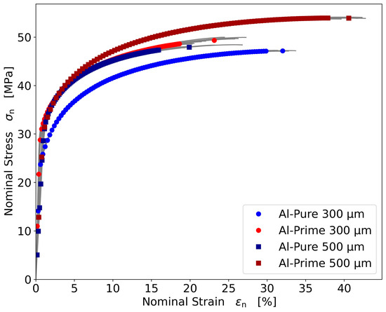
Figure 1.
Comparison of the average nominal stress–strain curves measured by tensile tests of Al-Pure (dark blue and blue) and Al-Prime (dark red and red) wires with diameters of 300 µm and 500 µm each.
The initial yield stresses of the individual wires are between 31 MPa and 32 MPa. The exception is the 300 µm Al-Pure wire with a lower initial yield stress of 24 MPa. This wire also has the lowest tensile strengths of 46 MPa, while the 500 µm diameter Al-Prime wire achieves the highest strength of 54 MPa. The tensile strengths of the thicker Al-Pure wire and the thinner Al-Prime wire are in between. The initial yield stresses and tensile strengths with standard deviations of all four wire types are summarized in Table 1.

Table 1.
Overview of the initial yield stress and the tensile strength of the four tested Al wires.
3.2. Fatigue Testing for Lifetime Modeling
The fatigue results of the Al-Pure wire with a diameter of 300 µm for the R-ratios from 0.1 to 0.7, which were presented in [27], were the starting point for the development of the fatigue lifetime model. But the results presented earlier needed to be extended and completed.
Compared to [27], stress amplitudes in the upper cycle range between 1000 and 10,000 cycles and further fatigue tests in the middle cycle range between 10,000 and 1,000,000 cycles were added to the measurement results. The complete fatigue results for Al-Pure with a diameter of 300 µm are shown in the following Wöhler diagram, Figure 2.
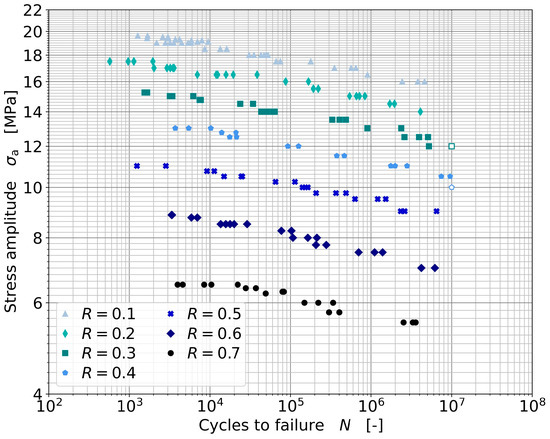
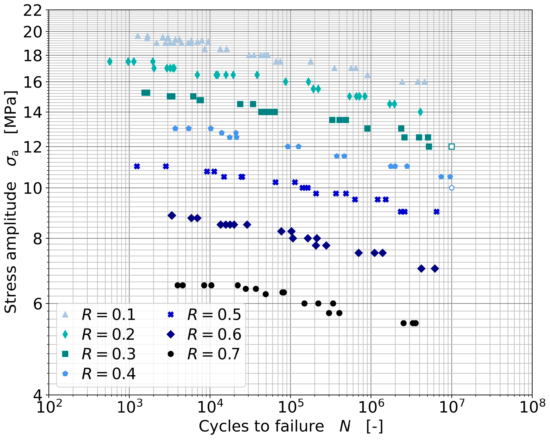
Figure 2.
Experimental fatigue results of Al-Pure with a diameter of 300 µm.
Due to the supplemented fatigue results and the smaller selected stress increments from = 0.50 to 0.25 MPa, the linear correlation in the double logarithmic plot of the individual Wöhler lines in the range of approximately 10,000 to 1,000,000 cycles is more noticeable for all investigated R-ratios. It becomes clear that the slope of the Wöhler lines flattens out for cycles below 10,000 and that this behavior becomes more pronounced with increasing R-ratio. It can be observed that the stress amplitudes decrease with increasing R-ratio and that the slope of the individual Wöhler lines increases at the same time. Two wire samples tested with R-ratios of 0.3 and 0.4 have withstood more than 10,000,000 cycles without failure and are therefore shown as unfilled markers.
3.3. Fatigue Lifetime Prediction Model
In the following sections, two possible approaches for lifetime modeling based on the fatigue results of the Al-Pure wire with a diameter of 300 µm are first calibrated and presented. Then, the modeling approaches are applied to the fatigue results of the other wire types. For this purpose, a scaling term is added to the models to include the tensile strength of the respective wire. The suitability of both models is subsequently evaluated. The modeling approaches are based on two equations from the literature, which have been adapted accordingly.
3.3.1. Fit of the Experimental Fatigue Data
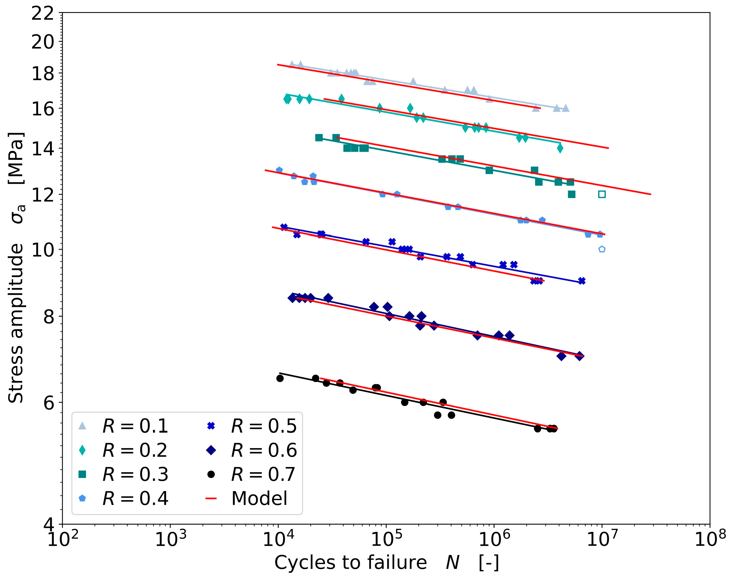
Due to the nearly linear relationship in the double logarithmic plot of the fatigue results in the range of 10,000 to 1,000,000 cycles, a linear approach is chosen for the initial modeling. Since the slope decreases for measurements below 10,000 cycles, these data are not considered by the authors when examining the linear approach. The Wöhler lines are fitted individually based on the Wöhler equation from the literature, see Equation (4).
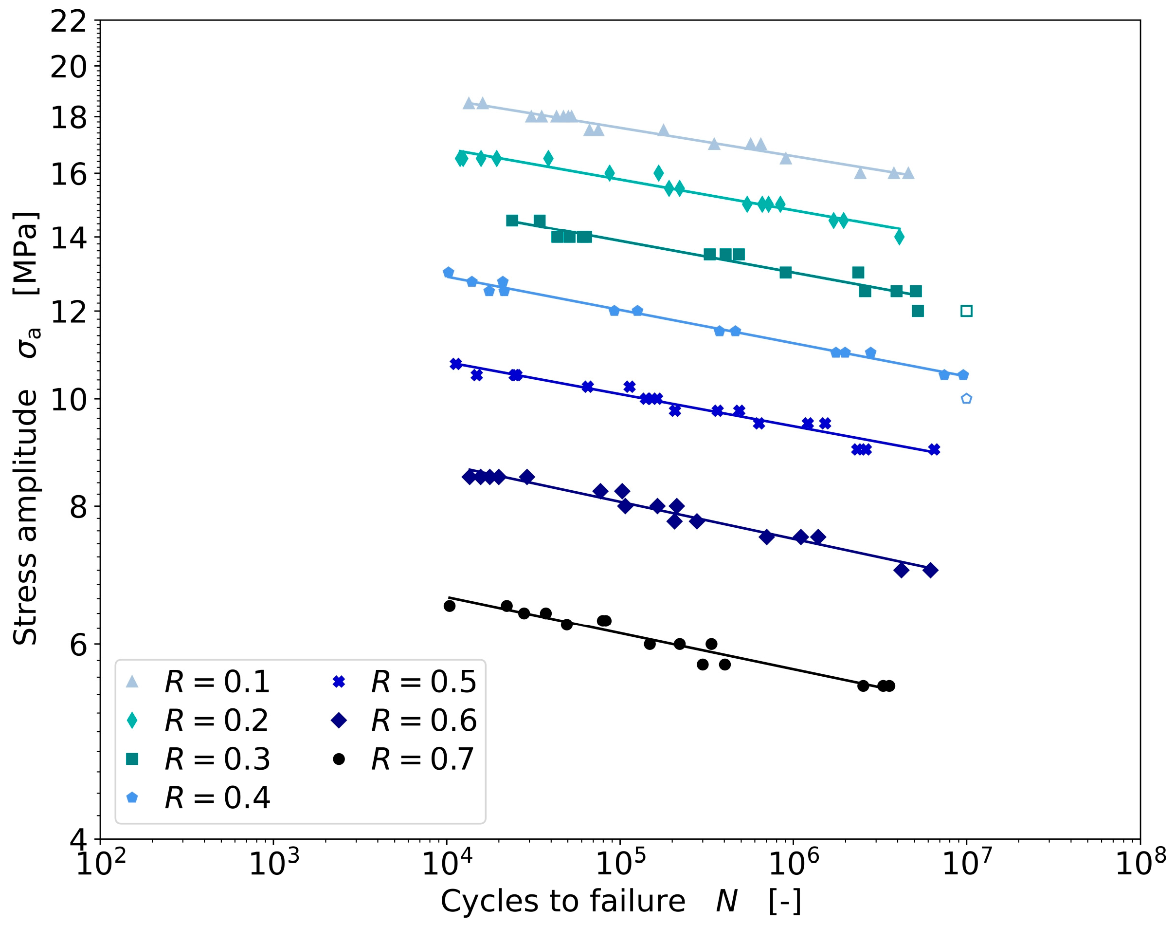
In contrast to the formula from the literature, the linear equation represents the dependence of the stress amplitude on the number of cycles until breakage in a double logarithmic plot. The linear fit function contains the two fit parameters and which represent the ordinate section and the slope. The reduced fatigue data of the Wöhler curves, including the linear regressions, are shown in Figure 3. It is shown that the reduced data is well represented by the linear Wöhler lines.

Figure 3.
Linear fit of the experimental fatigue data of Al-Pure with a diameter of 300 µm.
As a further possibility, a nonlinear approach is investigated. In this approach, all existing fatigue measurement results are used. To represent the transition to the low-cycle fatigue (LCF) range, the tensile strength is additionally considered in the model. For this, a transformation of the tensile strength to a corresponding stress amplitude for different stress ratios is necessary, see Equation (5).
For the nonlinear approach, the description based on Stüssi is used, this gives a sigmoid curve with transitions to the fatigue limit and the LCF range, see Equation (6) [30].
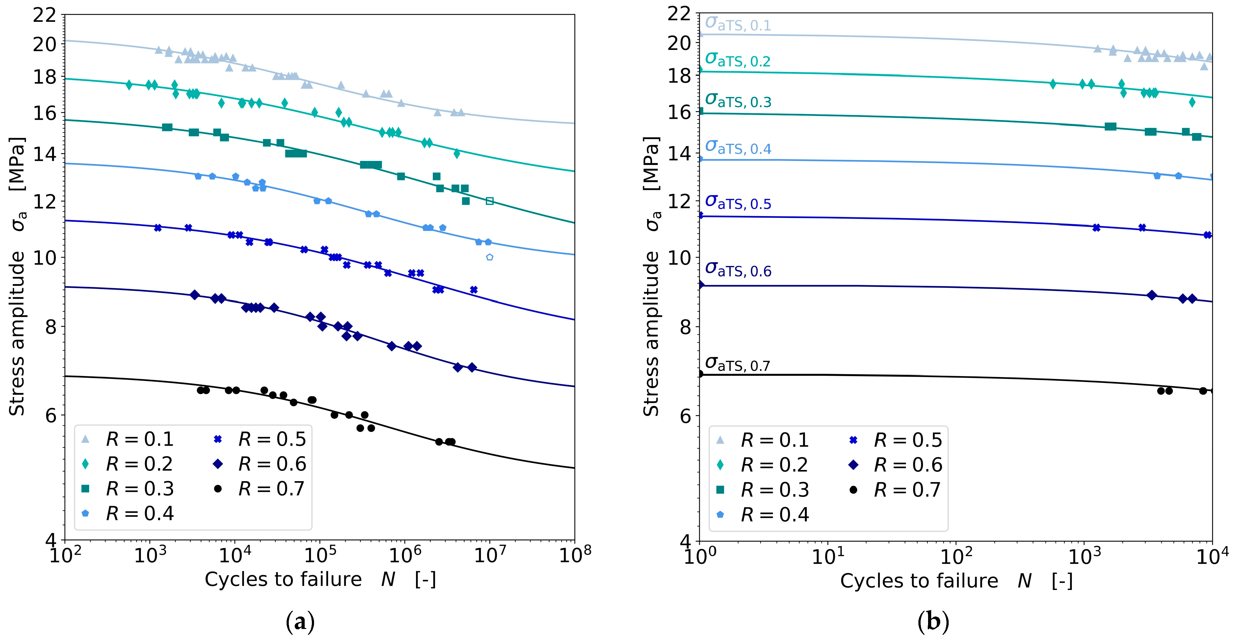
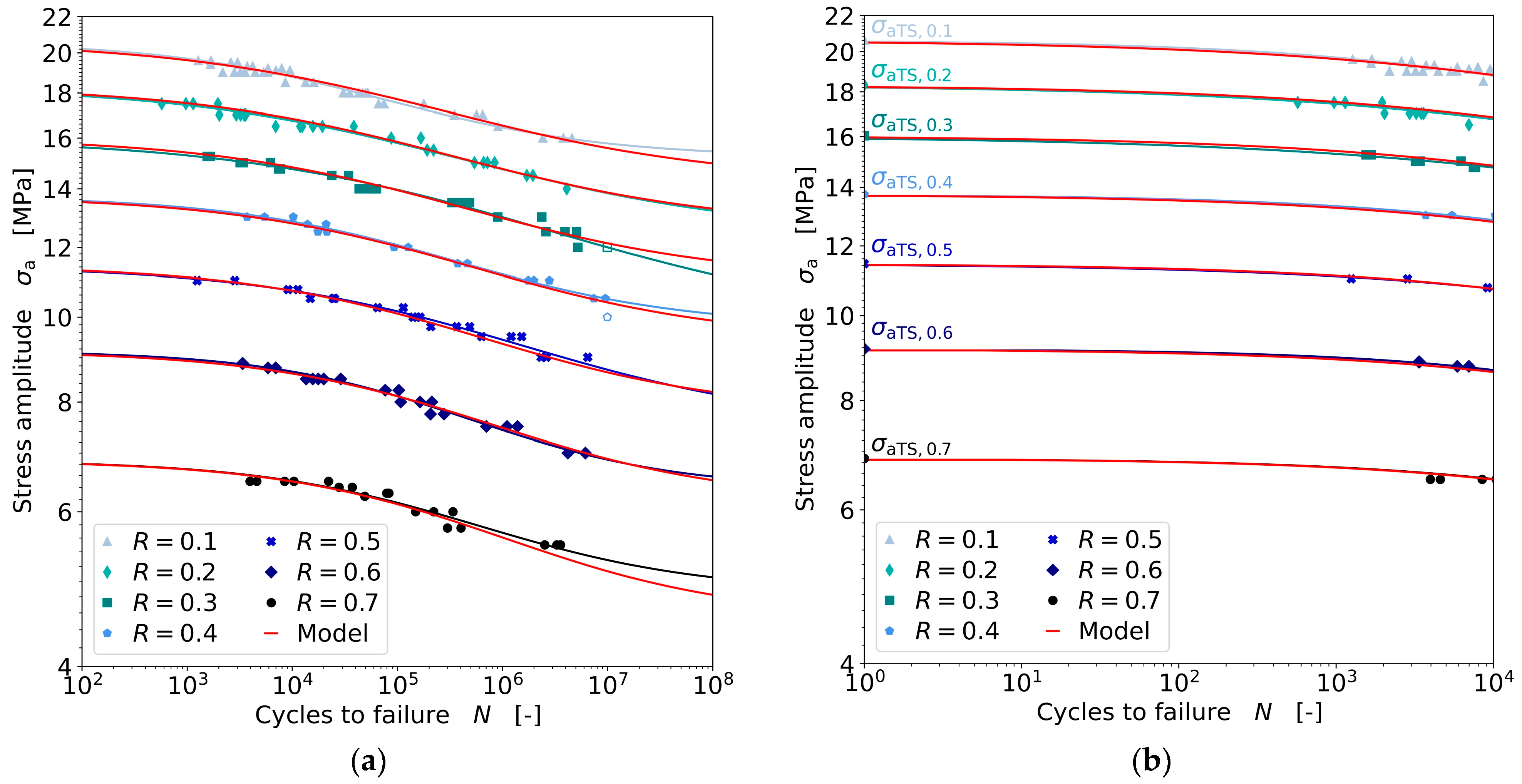
The nonlinear equation represents the dependence of the number of cycles to failure on the stress amplitude and the tensile strength converted to the stress amplitude in double logarithmic representation. The nonlinear fit function contains three fit parameters , and , where indicates the fatigue strength limit. The Wöhler lines fitted by the nonlinear approach according to Stüssi are shown in Figure 4a. The nonlinear fit function represents the collected fatigue data well for all R-ratios without large deviations. The transitions to the fatigue limits and the low-cycle fatigue ranges are also well represented. Except for the fatigue limit for R = 0.3, where the fit function shows a linearly decreasing trend. Figure 4b shows an enlarged section of the fit curves in the range from 1 to 1000 cycles for each Wöhler line. The stress amplitude calculated from the tensile strength is plotted for N = 1 in the diagram. is consistent with the experimental short-term fatigue results of each R-ratio.
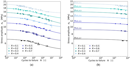
Figure 4.
Nonlinear fit of the experimental fatigue data of Al-Pure with a diameter of 300 µm (a), enlarged section of fatigue data with nonlinear fit in the range of 1 to 1000 cycles including the static stress amplitude (b).
3.3.2. Linear Lifetime Model
Based on the linearly fitted Wöhler lines, the lifetime modeling for the linear approach is performed next. For this purpose, the fit parameters and are determined for all Wöhler lines, plotted as a function of the R-ratios, and then fitted with model functions. For the fit of the model parameters, a quadratic function was chosen for , see Equation (7), and a linear function was chosen for , see Equation (8).
, , and , are the corresponding parameters for fitting and . The results of the fitted model parameters as a function of the R-ratio are shown in Figure 5a,b.
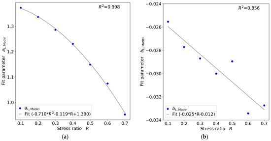
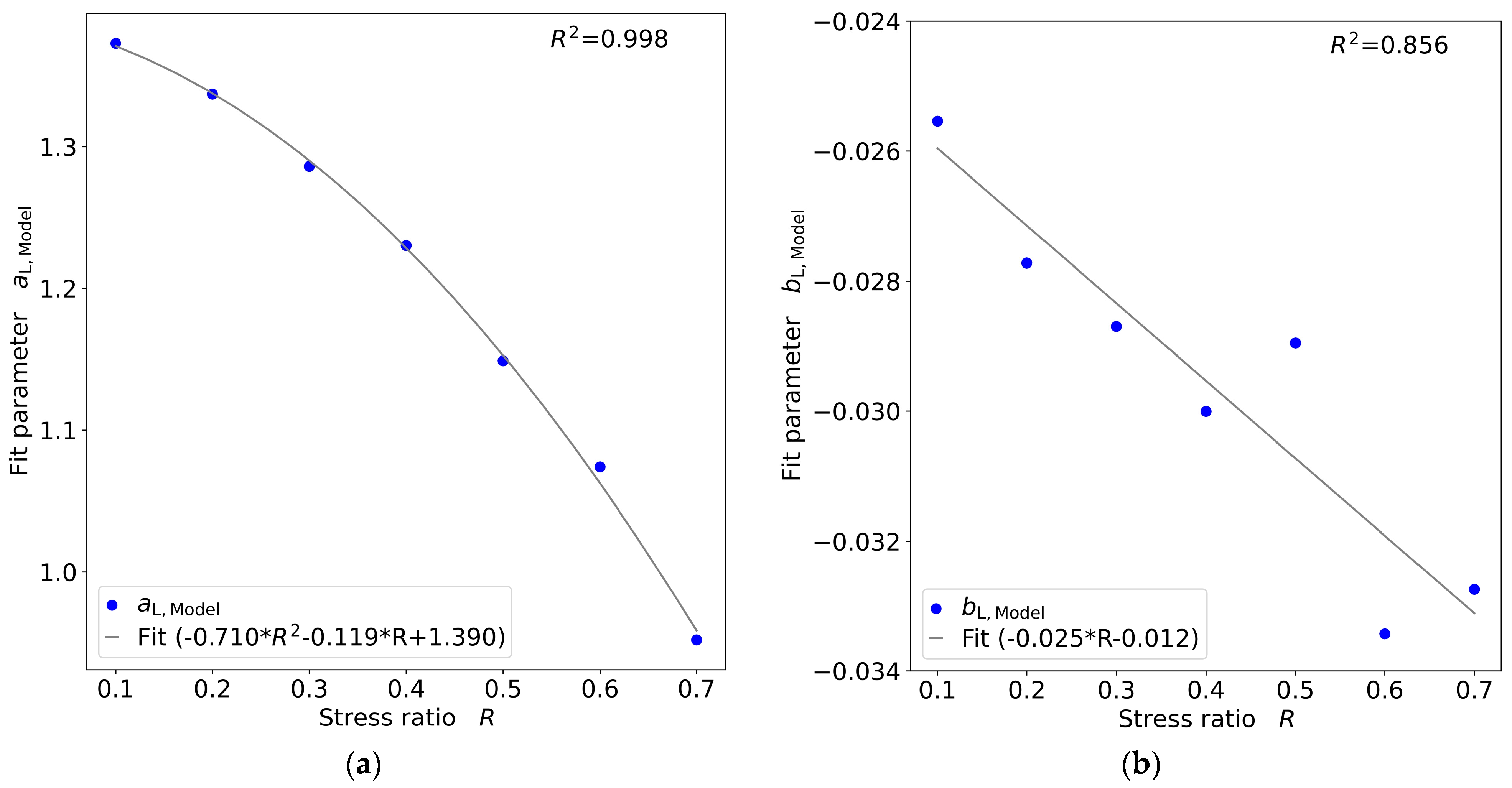
Figure 5.
Fit of the model parameters (a) and (b) as a function of the R-ratio for the linear fatigue lifetime model.
As can be seen from Figure 5a, which shows the fitting of the respective ordinate sections , these can be plotted well with the quadratic function. The individual model parameters hardly deviate from the curve, which can also be illustrated by the high coefficient of determination R2 of 0.998. It also shows that decreases with the increasing R-ratio.
For parameter in Figure 5b, which shows the fitting of the respective slopes, the selected linear fitting function also fits the values well. However, the values for R = 0.5 and R = 0.6 are slightly further away from the fitted straight line. The values for the other five R-ratios are very close to the fit. The coefficient of determination R2 of 0.856 is therefore lower than that of the ordinate section.
After fitting the parameters and , the two fit model functions are inserted into the linear lifetime fatigue model equation and rearranged according to the model number of cycles until breakage , see Equation (9).
After applying the model equation, the fatigue behavior shown in Figure 6 can be predicted for the individual R-ratios for the linear fatigue lifetime model (in red). For better comparability, the results for the linear fit from Figure 3 are also shown.
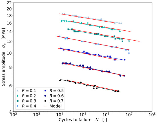
Figure 6.
Linear fatigue lifetime model calibrated and applied to Al-Pure with a diameter of 300 µm.
The results of the linear fatigue lifetime model show a very good agreement between linear regression and model curves; see Figure 6. The positions of the model lines are in good agreement with the positions of the fit curves, which is due to the large correlation between the model parameter and the R-ratio; see Figure 5a. The model curves for the R-ratios 0.1, 0.5 and 0.7 show slightly larger slopes than the fit curves. This observation correlates with the fitted slope values of the model parameter ; see Figure 5b. The agreement of the model is also examined by calculating the relative deviations of the logarithm of the cycles to failure between all experimental data points and the corresponding model data, see Equation (3). The mean relative deviation between model and experiment is 3.4%, and the maximum relative deviation is 8.3%, which illustrates the very good agreement between the model and the experimental data.
Since not all collected data points are considered in the modeling, an additional comparison is made with the relative deviations of all data points, including the measured data below 10,000 cycles. Here, the mean relative deviation increases to 5.2%, and the maximum relative deviation increases to 16.4%. This indicates that limiting the data for the linear model is necessary, and the linear model should not be applied below 10,000 cycles.
3.3.3. Nonlinear Lifetime Model
Based on the nonlinearly fitted Wöhler lines, the lifetime modeling for the nonlinear approach is performed next. For this purpose, the fit parameters , and are determined for all Wöhler lines, plotted as a function of the R-ratio, and then fitted with model functions. Three linear functions are used to fit the parameters , and , see Equations (10)–(12).
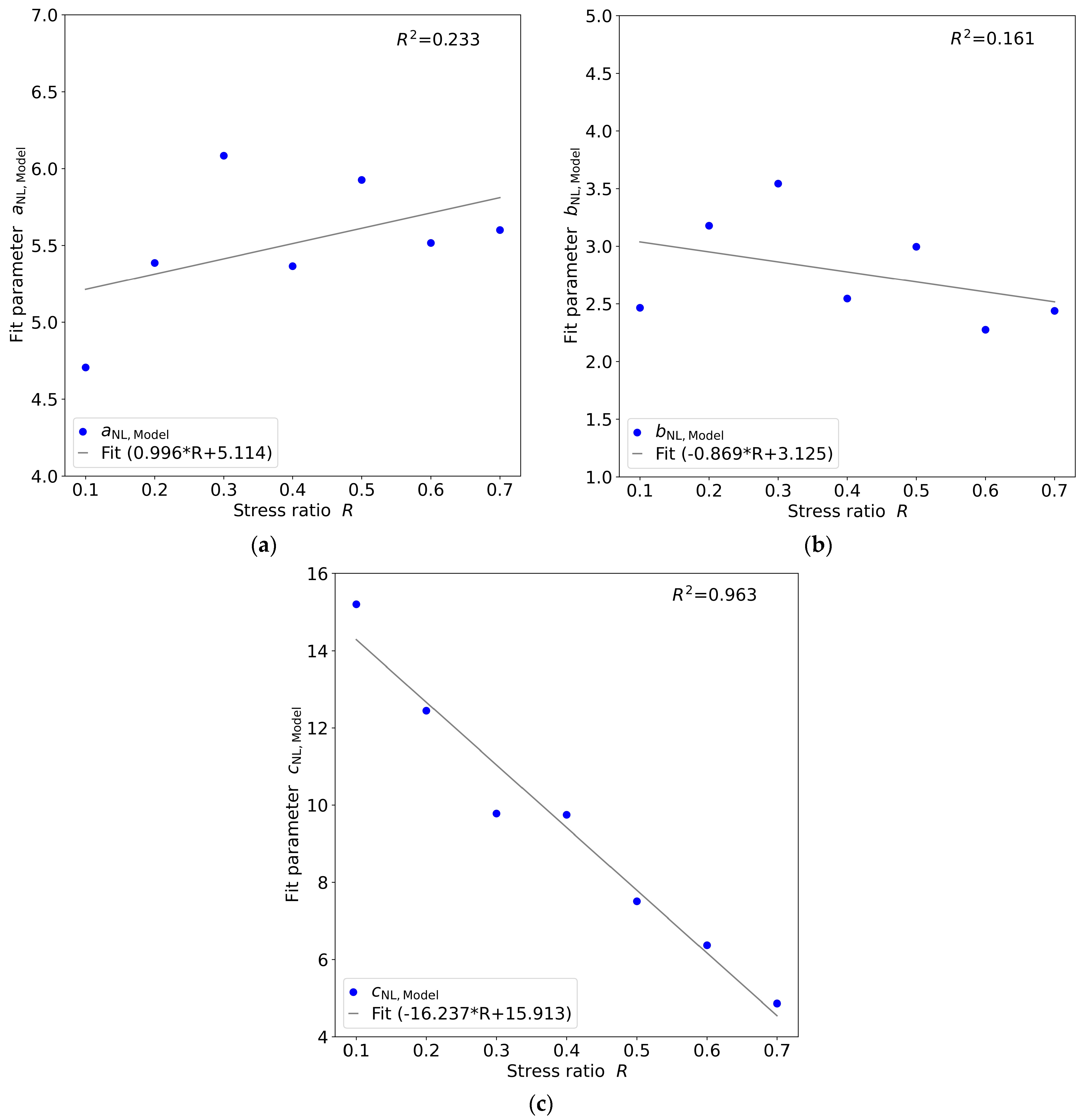
, , , and , are the corresponding fit parameters for fitting , and . The results of the fitted parameters as a function of the R-ratio are shown in Figure 7a–c.
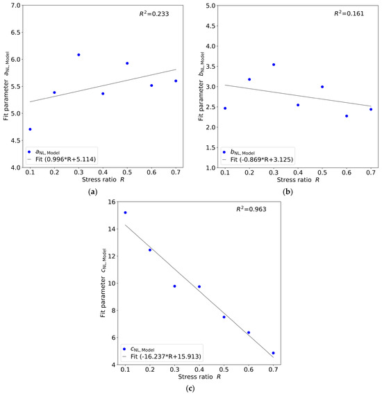
Figure 7.
Fit of the fit parameters (a), (b) and (c) as a function of the R-ratio of the nonlinear fatigue lifetime model.
From the plot of the fitting function of , see Figure 7a, there is a relatively large deviation of the individual vales in a small range. For this reason, there appears to be very little or no correlation between the model parameter and the R-ratio. In general, the model values show a low increasing tendency with increasing R-ratio, which can be approximated by a linear fitting function. The low correlation with a slight increase in the model values can be further evidenced by the Pearson correlation coefficient, which is 0.34. A similar conclusion can be drawn for the model parameter ; see Figure 7b. The model values there also deviate relatively large in a small range, so that a correlation with the R-ratio is relatively low. However, the model values of show a slightly decreasing trend with increasing R-ratio, which can be approximately reproduced by a linear fitting function. The low correlation with a slight decrease in the model values can be further evidenced by the Pearson correlation coefficient, which is −0.31. These findings are also reflected in the very low coefficients of determination of the two model parameters. In contrast, the model value , which represents the fatigue strength limit, shows a high correlation with the R-ratios, see Figure 7c. The individual values show almost no deviations from the linear fit function, which is also shown by the very high R2 values of 0.963.
Then, the fitted model parameters , and are substituted into the nonlinear fatigue lifetime model equation according to Stüssi, see Equation (13).
After applying the model equation, the fatigue behavior shown in Figure 8a,b can be predicted for the individual R-ratios (in red) for the nonlinear fatigue lifetime model. For better comparability, the results for the nonlinear fit from Figure 4a,b are also shown.
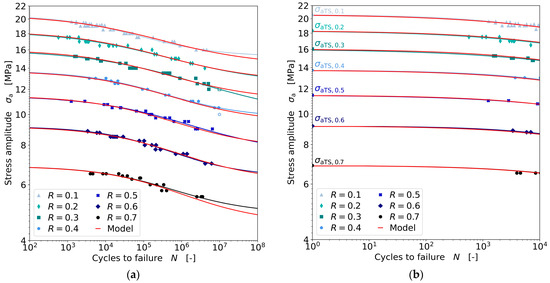
Figure 8.
Nonlinear fatigue lifetime model calibrated and applied to Al-Pure with a diameter of 300 µm (a), enlarged section of the nonlinear fatigue lifetime model in the range of 1 to 1000 cycles including the static stress amplitude (b).
The developed nonlinear fatigue lifetime model (see Figure 8a) shows a very good agreement for all R-ratios over the entire cycle range considered. A quantitative comparison of the experimental data with the model data using Equation (3) gives a mean relative deviation of 0.16% and a maximum relative deviation of 3.7%. These very small deviations illustrate the very good agreement between the nonlinear model and the experimental data. Thus, it can be shown that the apparently low correlation between the model parameters and and the R-ratio does not have a major impact on the representation of the nonlinear fatigue lifetime model. For the fatigue limit range, there are small deviations between the fitting curves and the model curves for the R-ratios of 0.1, 0.3 and 0.7. Since there is a very large correlation between the model parameter and the R-ratio, it can be assumed that the prediction of the nonlinear fatigue lifetime model in the fatigue limit range is more credible than the prediction of the individual fitted curves. Presumably, too few data points are available in the maximum cycle range for a reliable extrapolation to the fatigue limit for the individual fits. The values of the tensile strength in the low-cycle fatigue range, which are converted into the stress amplitude , are well matched by all model curves; see Figure 8b.
3.4. Verification of the Extrapolation by Smith Diagrams
After applying the models to the Al-Pure wire with a diameter of 300 µm, which have already shown good agreement, the next step is to check whether it is possible to extrapolate the model data using Smith diagrams with 1,000,000 cycles each. For this purpose, the models are extrapolated over an R-ratio range from −1.0 to 0.8.
First, the experimental fatigue results are compared with the linear fatigue lifetime model results (see Figure 9). The experimental results are obtained from the linear fitting equations of the individual R-ratios by calculating the corresponding maximum and minimum stresses for 1,000,000 cycles. The modeled results are determined based on the linear lifetime fatigue model equation for the different R-ratios to determine the modeled maximum and minimum stresses for 1,000,000 cycles.
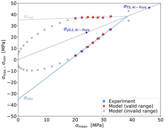
Figure 9.
Smith diagram for 1,000,000 cycles with experimental data (blue) for the R-ratios from 0.1 to 0.7 including linear extension of Smith lines (blue) and model data (grey, red) for R-ratios from −1.0 to 0.8.
Figure 9 shows an adapted Smith diagram according to [27] with the experimental results for the R-ratios from 0.1 to 0.7 (blue) and the linear extensions of the Smith lines. All maximum stress values for 1,000,000 cycles are significantly above the initial yield stress of the wire, so that massive plastic deformation and necking accompany the fatigue failure. More information about the failure mechanism and fracture appearance is shown in [27]. The Smith diagram is complemented by the modeled maximum and minimum stress values for the R-ratios from −1.0 to 0.8. The modeled stress values for the R-ratios from 0.1 to 0.7 (red) are very similar to the experimental results and reproduce them well. The remaining modeled R-ratios above or below the range of 0.1 to 0.7 (grey) will not be correctly predicted by the current linear fatigue life model. The R-values below 0.1 do not run along the linearly extended Smith lines but are elliptically below the maximum stress line and above the minimum stress line. Above an R-ratio of 0.7, the maximum and minimum stress values run parallel to the diagonal line without approaching an intersection point. The Smith diagram is therefore limited to a maximum R-ratio of 0.7.
The reason that the interpolation between the R-ratios 0.1 and 0.7 fits very well and the extrapolation does not is due to the fitting equations chosen for the parameters and . The quadratic function of the ordinate intercept has a particularly large effect on the shape of the model predictions because it has a parabolic shape, as can be seen for the R-ratios below 0.1. In contrast, the fit equation for the slope has a linear form and thus a smaller influence. If instead of the quadratic function for also a linear function as for is assumed, the Wöhler lines of the model show very large deviations and partly shift to the fit functions. Also, a representation in the Smith diagram results in considerable deviations, which is why a graphical representation is omitted here. The model presented here is therefore only applicable to a range from R = 0.1 to R = 0.7.
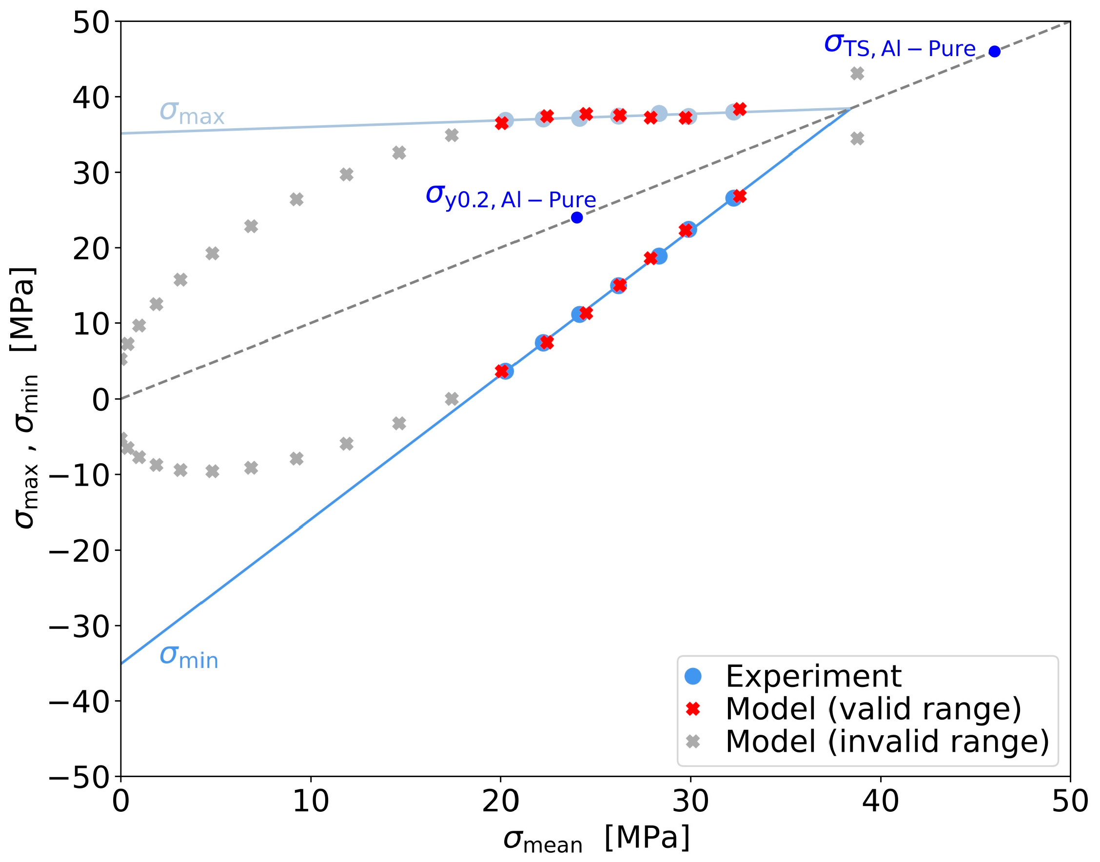
Subsequently, the experimental fatigue results are compared with the results of the nonlinear fatigue lifetime model (see Figure 10). The experimental results are calculated in the same way as described for the linear model. The modeled results are calculated by the nonlinear fatigue lifetime model equation for the different R-ratios to determine the modeled maximum and minimum stresses for 1,000,000 cycles.
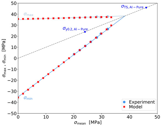
Figure 10.
Smith diagram with 1,000,000 cycles with experimental data (blue) for the R-ratios from 0.1 to 0.7 and with model data (red) for the R-ratios from −1.0 to 0.8 based on the nonlinear fatigue lifetime prediction model.
Figure 10 shows an extended Smith diagram based on [27] with the experimental results for the R-ratios from 0.1 to 0.7 (blue), supplemented by the modeled maximum and minimum stress values for the R-ratios from −1.0 to 0.8 (red). The model values provide very consistent results both in the experimentally detectable range from 0.1 to 0.7 and show a linear progression above and below this range. The model shows the expected linear behavior of the maximum and minimum stress lines very well even outside the experimental range. The reason for this is the chosen curve shape of the fitting functions for the three parameters , and , which each indicate the course of a straight line. The progression of maximum and minimum stress values for additional R-ratios appears reasonable and opens the possibility of predicting the fatigue lifetime behavior for specific R-ratios based on the presented results and modeling without further experimental investigations.
3.5. Transfer of the Fatigue Models to Further Aluminum Bonding Wires
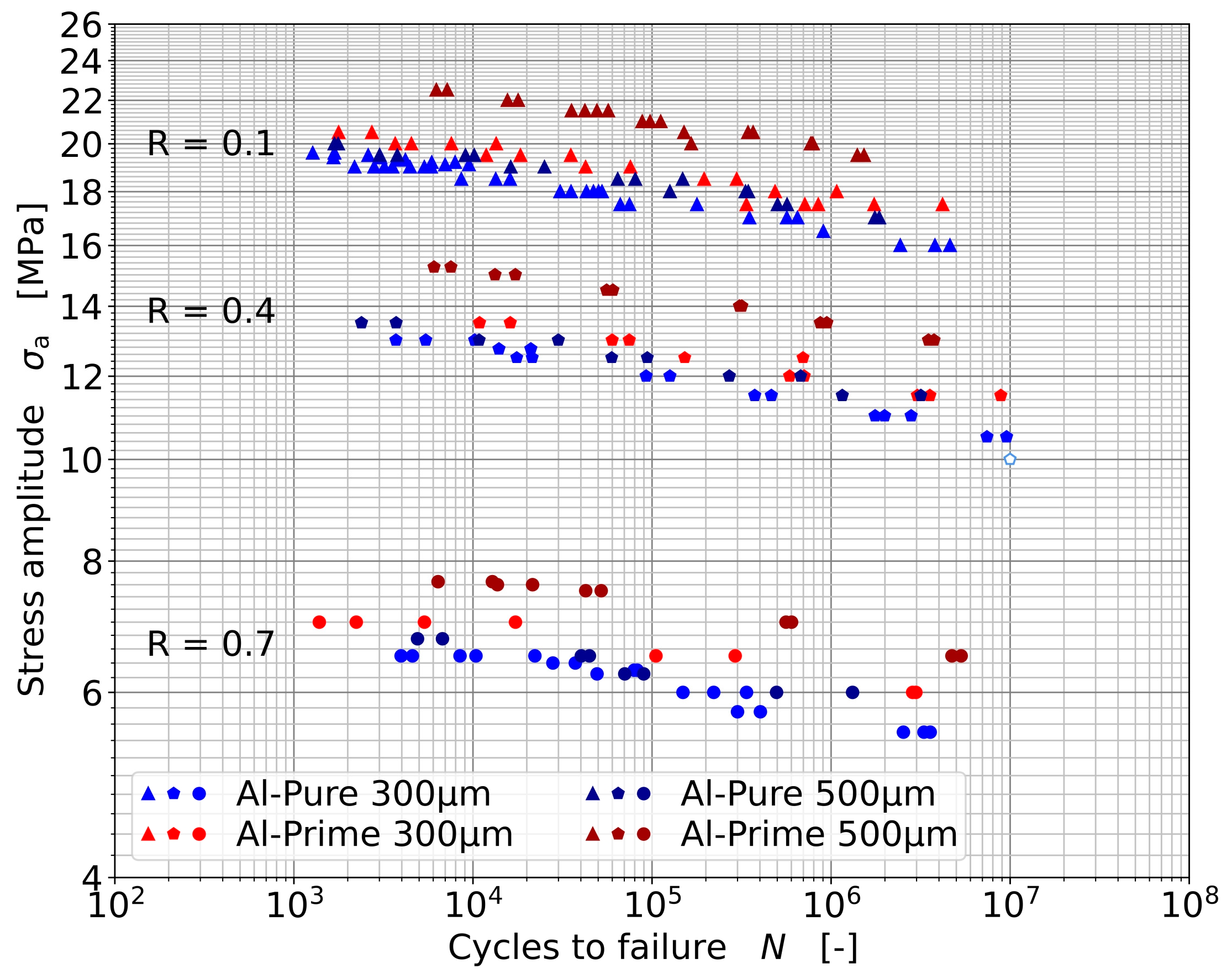
After developing and presenting the two different approaches for modeling the fatigue lifetime behavior based on the Al-Pure wire with a diameter of 300 µm, the next step is to apply the two models to the fatigue results for the other three wire types. For this purpose, the fatigue behavior of the wires was determined experimentally for the three R-ratios of 0.1, 0.4 and 0.7 (see Figure 11). Here, the results of the individual Wöhler tests for the three R-ratios are approximately linear and parallel to each other. The Al-Prime wire with a diameter of 500 µm (dark red) achieves the highest stress amplitudes. The results of this wire type are clearly above those of the other wires investigated for all R-ratios. The results of the same wire type with a diameter of 300 µm (red) are about 1–2 MPa below the stress amplitudes of the Al-Prime with a diameter of 500 µm. Directly below this are the results of the Al-Pure with a diameter of 500 µm (dark blue). These are very close to the results of the Al-Prime with a diameter of 300 µm, so that they partially overlap. Finally, with the lowest stress amplitudes, follow the results of the Al-Pure with a diameter of 300 µm, which have been used to calibrate the two fatigue lifetime approaches (blue). The order of the fatigue results of all four wire types according to their occurring strengths can be very well related to the results of their tensile tests; see Figure 1.
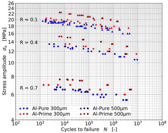
Figure 11.
Experimental fatigue results of Al-Pure (dark blue and blue) and Al-Prime (dark red and red) with diameters of 300 µm and 500 µm at R-ratios of 0.1, 0.4 and 0.7.
Subsequently, both model approaches are applied to the fatigue results with R-ratios of 0.1, 0.4 and 0.7 for another wire. For this purpose, the stress amplitude must be scaled to the quotient of the tensile strength of the Al-Pure with a 300 µm diameter and the tensile strength of the other wire (see Equation (14)).
The scaled stress amplitude can then be substituted for the stress amplitude in both model equations, allowing the prediction of Wöhler lines for different R-ratios based on the tensile strength of the wire in question. For the linear modeling of the wire fatigue lifetime, the following Equation (15) is obtained.
The nonlinear fatigue lifetime model replaced by the scaled stress amplitude is shown in Equation (16).
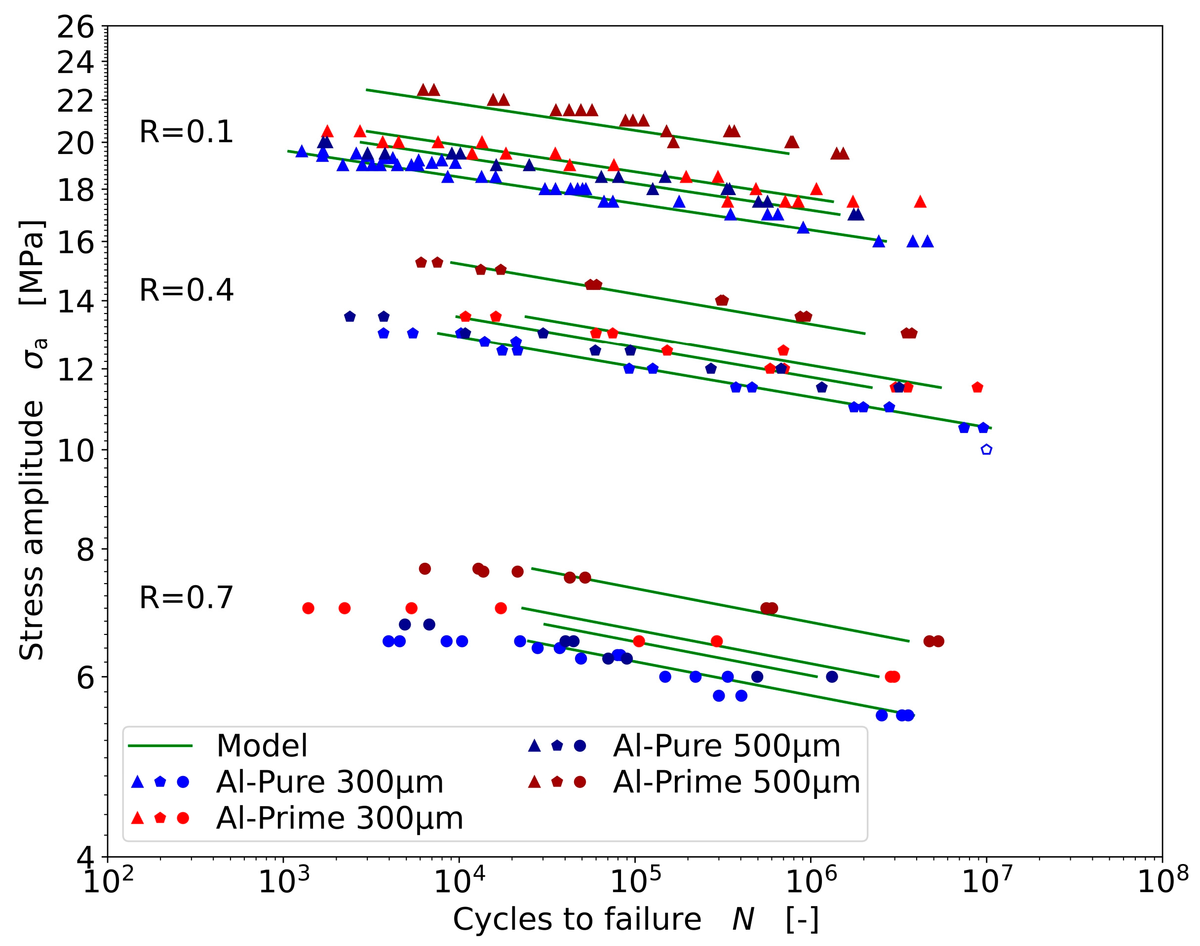
Figure 12 shows the fatigue results with the linearly modeled Wöhler lines (in green) for all four wire types investigated. To verify that the predicted model lines are accurate, the experimental results of the wires are also plotted on the Wöhler diagram.
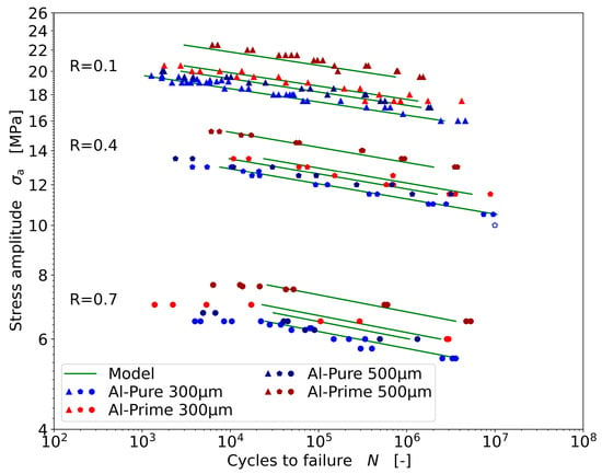
Figure 12.
Linear fatigue lifetime model (green) applied to Al-Pure and Al-Prime with diameters of 300 µm and 500 µm for the R-ratios of 0.1, 0.4 and 0.7.
The model lines of the linear fatigue lifetime model show good agreement with the experimental results of all four wire types. All experimentally measured values were considered when applying the linear model, and the measured values below 10,000 cycles were not neglected as in the calibration of the model (compare Figure 3). Here, especially the larger stress amplitudes at higher R-ratios, cannot be well reproduced by the linear model. The agreement of the applied model with the experimental data is also investigated by a quantitative comparison of the relative deviations with and without the data below 10,000 cycles using Equation (3). The mean relative deviation based on all data is 6.0% and the maximum relative deviation is 15.5%, while the mean relative deviation based on the reduced data is 4.2% and the maximum relative deviation is 8.8%.
Thus, the linear fatigue lifetime model can only be used to represent the linear range of the Wöhler line and not the entire cycle range. However, the model is very well suited for the linear Wöhler range, as shown by the low relative deviations between model and experiment. Compared to the developed model, the model applied to other wire materials shows slightly larger deviations, except for the maximum relative deviation related to all data points.
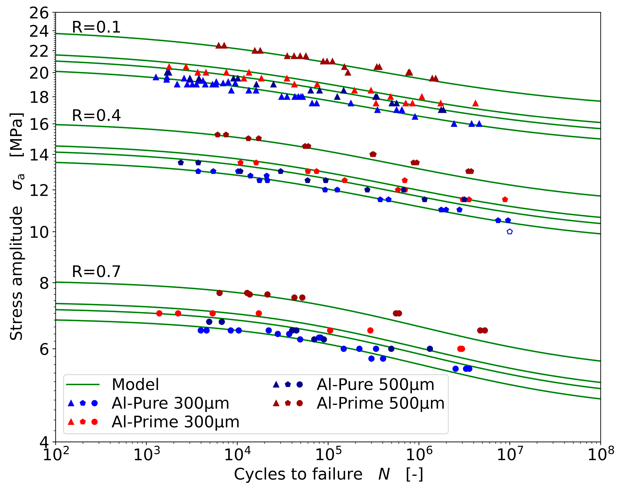
Next, the nonlinear fatigue lifetime model is applied to the experimental fatigue results of the four wire types, see Figure 13.
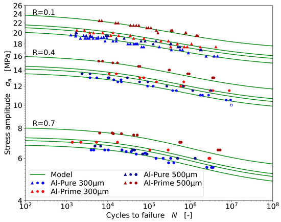
Figure 13.
Nonlinear fatigue lifetime model (green) applied to Al-Pure and Al-Prime with diameters of 300 µm and 500 µm for the R-ratios of 0.1, 0.4 and 0.7.
The nonlinear model can reproduce the entire cycle range considered very well for all four wires. This is also verified by a low mean relative deviation of 0.42% and a low maximum relative deviation of 5.1%. The relative deviations of the model applied to the other wires are only slightly larger than the relative deviations of the developed model. Smaller differences occur in the fatigue results of the Al-Prime wire with a diameter of 500 µm and show small deviations from the model lines and the experiment for the R-ratio of 0.7 in the transition region from high-cycle fatigue (HCF) to the fatigue strength limit. Here, the experimental data run slightly above the model line, while the first measurement points can be represented very well by the model. The reason for the deviations could be the small amount of experimental data for the other wires. While for the modeling, the data sets for the Al-Pure wire with a diameter of 300 µm were further supplemented to be able to generate the models more accurately, for the other wire types investigated, mostly only double determinations were carried out for the individual stress. Supplementary measurements can contribute to the higher accuracy.
4. Discussion
In the presented paper, a linear and a nonlinear fatigue lifetime model were developed and calibrated based on fatigue results from a 300 µm Al-Pure aluminum bonding wire in a double logarithmic representation. Two fatigue equations from the literature were used as the basis for the modeling, with which the experimental results were fitted in a first step, and their parameters were fitted and transferred to the model equations for the fatigue life predictions in a second step. The two modeling approaches were subsequently applied to other aluminum wire types and diameters to verify that the tensile strength of the wires could be used to predict their fatigue behavior. For this purpose, a scaling term was added to the models to account for the tensile strength of the wire.
The linear fatigue lifetime model is based on the Wöhler equation and showed good reproducibility on plotting the individual Wöhler lines above 10,000 cycles for R-ratios of 0.1 to 0.7. However, the model could not be applied below 10,000 cycles and outside the R-ratio range. Since only a straight line could be modeled in the Wöhler diagram, the lower cycle range could not be modeled with this model because of its decreased slopes. This is also evidenced by the increasing mean and maximum relative deviations when the cycles below 10,000 are included in the calculations. In the associated Smith diagram for 1,000,000 cycles, only the experimentally detectable range of 0.1 to 0.7 was well reproduced because of the shape of the fitting equations for the model parameters. The model could be transferred to the other wires by scaling to their strength and representing well the cycles over 10,000 of the other wires. Outside this range, however, the model was not applicable.
The nonlinear fatigue lifetime model is based on the Stüssi equation and showed very good reproducibility in plotting the Wöhler lines over the entire cycle range studied. The model reproduced the entire Wöhler curve very well and showed only very small deviations between model and experimental data. The Smith diagram for 1,000,000 represented the R-ratios from 0.1 to 0.7 very well and allowed very reasonable predictions for the further R-ratios. The nonlinear model could therefore be used for the entire cycle range considered, as well as for all R-ratios between −1.0 and 0.8.
The nonlinear model could be transferred very well to the other aluminum wires. The mean relative deviation of 0.42% and the maximum relative deviation of 5.1% provide higher accuracy for the applied nonlinear model than the applied linear model, where the mean relative deviation is 4.2% and the maximum relative deviation is 8.8%. For this reason, the nonlinear model is to be preferred for lifetime prediction.
With these results, it could be confirmed that a general room-temperature fatigue life model could be developed and that it was possible to predict the fatigue behavior of a wire based on the knowledge of its tensile strength. However, the model currently does not consider temperature, microstructure, frequency, or other loading situations. Some investigations in the literature have shown that these boundary conditions can affect the fatigue behavior of the wires [5,6,7,14,15,16,17,18,21,22]. Further investigations in address these influences are planned. Another aspect, that can be relevant for the lifetime of bonded wire bridges is the ultrasonic loading during the bonding process and the bending during the bridge formation. These process-related aspects will not be considered since we want to separate pure material behavior as a first step.
Author Contributions
Conceptualization, C.M. and C.D.; methodology, C.M. and C.D.; software, C.M. and C.D.; validation, C.M. and C.D.; formal analysis, C.M.; investigation, C.M.; resources, C.M. and C.D.; data curation, C.M. and C.D.; writing—original draft preparation, C.M.; writing—review and editing, C.M., C.D. and H.A.; visualization, C.M. and C.D.; supervision, C.D. and H.A.; project administration, C.D.; funding acquisition, C.D. All authors have read and agreed to the published version of the manuscript.
Funding
This research was partially funded by the German Federal Ministry of Education and Research in the project WireLife in the program FH-Kooperativ under the funding code 13FH544KX0, by the Graduate Institute of the University of Applied Science Bonn-Rhein-Sieg and the Institute of Technology, Resource and Energy-efficient Engineering.
Data Availability Statement
The data presented in this study are available on request from the corresponding authors.
Acknowledgments
We would like to thank the project partner Heraeus Deutschland GmbH Co. KG for providing the wire materials.
Conflicts of Interest
The authors declare no conflict of interest. The funders had no role in the design of the study; in the collection, analyses, or interpretation of data; in the writing of the manuscript; or in the decision to publish the results.
References
- Altenbach, H.; Dresbach, C.; Petzold, M. Characterizing the Anisotropic Hardening Behavior of Aluminum Bonding Wires. In Materials with Complex Behaviour II; Öchsner, A., Da Silva, L.F.M., Altenbach, H., Eds.; Springer-Verlag: Berlin/Heidelberg, Germany, 2012; pp. 583–598. [Google Scholar]
- Li, L.; Xu, S.; Liang, Y.k.; Wie, P. 10 mils Al wire heavy wedge bond wire deformation thickness study. In Proceedings of the 20th International Conference on Electronic Packaging Technology (ICEPT), Hong Kong, China, 12–15 August 2019. [Google Scholar]
- Levine, L. Wire Bonding. EDFAAO 2016, 18, 22–28. [Google Scholar] [CrossRef]
- Treto, R.; Kim, G. Optimization of Ultrasonic Aluminum Wire Bonding on Chromium and Gold Surfaces Using K&S Wedge Wire Bonder; Sing Center for Nanotechnology: Philadelphia, PA, USA, 2019. [Google Scholar]
- Merkle, L.; Kaden, T.; Sonner, M.; Gademann, A.; Turki, J.; Dresbach, C.; Petzold, M. Mechanical fatigue properties of heavy aluminium wire bonds for power applications. In Proceedings of the 2nd Electronics Systemintegration Technology Conference (ESTC), Greenwich, UK, 1–4 September 2008; pp. 1363–1368. [Google Scholar]
- Merkle, L.; Sonner, M.; Petzold, M. Lifetime prediction of thick aluminium wire bonds for mechanical cyclic loads. Microelectron. Reliab. 2014, 54, 417–424. [Google Scholar] [CrossRef]
- Merkle, L.; Sonner, M.; Petzold, M. Developing a model for the bond heel lifetime prediction of thick aluminium wire bonds. Solder. Surf. Mt. Technol. 2012, 24, 127–134. [Google Scholar] [CrossRef]
- Bai, C.; Fan, J.; Qian, C.; Guo, W.; Fan, X.; Zhang, G. Electrical-thermo-mechanical Simulation for Aluminum Wire Bonds in Sic Schottky Diode Packages. In Proceedings of the 2016 IEEE 13th China International Forum on Solid State Lighting: International Forum on Wide bandgap Semiconductors China (SSSLChina: IFWS), Beijing, China, 15–17 November 2016. [Google Scholar]
- Ciappa, M. Selected failure mechanism of modern power modules. Microelectron. Reliab. 2002, 42, 653–667. [Google Scholar] [CrossRef]
- Czerny, B.; Paul, I.; Khatibi, G.; Thoben, M. Experimental and analytical study of geometry effects on the fatigue life of Al bond wire interconnects. Microelectron. Reliab. 2013, 53, 1558–1562. [Google Scholar] [CrossRef]
- Wright, A.; Hutzler, A.; Schletz, A.; Pichler, P. Thermo-mechanical simulation of plastic deformation during temperature cycling of bond wires for power electronic modules. In Proceedings of the 2014 IEEE 15th International Conference on Thermal, Mechanical and Multi-Physics Simulation and Experiments in Microelectronics and Microsystems (EuroSimE), Ghent, Belgium, 7–9 April 2014. [Google Scholar]
- Jiang, N.; Scheibel, M.G.; Fabian, B.; Kalajica, M.; Miric, A.-Z.; Lutz, J. Effects of Inorganic Encapsulation on Power Cycling Lifetime of Aluminum Bond Wires. In Proceedings of the 30th International Symposium on Power Semiconductor Devices & ICs (ISPSD), Chicago, IL, USA, 13–17 May 2018; pp. 244–247. [Google Scholar]
- Packwood, M.; Li, D.; Mumby-Croft, P.; Dai, X. Thermal Simulation into the Effect of Varying Encapsulant Media on Wire Bond Stress Under Temperature Cycling. In Proceedings of the 2018 IEEE 19th International Conference on Electronic Packaging Technology (ICEPT), Shanghai, China, 8–11 August 2018; pp. 152–155. [Google Scholar]
- Czerny, B.; Khatibi, G. Accelerated mechanical fatigue interconnect testing method for electrical wire bonds. Tm-Tech. Mess. 2018, 85, 213–220. [Google Scholar] [CrossRef]
- Czerny, B.; Khatibi, G. Cyclic robustness of heavy wire bonds: Al, AlMg, Cu and CucorAl. Microelectron. Reliab. 2018, 88–90, 745–751. [Google Scholar] [CrossRef]
- Czerny, B.; Khatibi, G. Highly accelerated mechanical lifetime testing for wire bonds in power electronics. J. Microelectron. Electron. Packag. 2022, 19, 49–55. [Google Scholar] [CrossRef]
- Broll, M.S.; Geissler, U.; Höfer, J.; Schmitz, S.; Wittler, O.; Lang, K.D. Microstructural evolution of ultrasonic-bonded aluminum wires. Microelectron. Reliab. 2015, 55, 961–968. [Google Scholar] [CrossRef]
- Halouani, A.; Khatir, Z.; Shqair, M.; Ibrahim, A.; Pichon, P.-Y. An EBSD study of fatigue crack propagation in bonded aluminum wires cycled from 55 °C to 85 °C. J. Electron. Mater. 2022, 51, 7353–7365. [Google Scholar] [CrossRef]
- Loh, W.-S.; Corfield, M.; Lu, H.; Hogg, S.; Tilford, T.; Johnson, C.M. Wire Bond Reliability for Power Electronic Modules—Effect of Bonding Temperature. In Proceedings of the 2007 IEEE Thermal, Mechanical and Multipyhsics Simulation and Experiments in Micro-Electronics and Micro-Systems (EuroSimE), London, UK, 16–18 April 2007. [Google Scholar]
- Dornic, N.; Ibrahim, A.; Khatir, Z.; Degrenne, N.; Mollov, S.; Ingrosso, D. Analysis of the aging mechanism occurring at the bond-wire contact of IGBT power devices during power cycling. Microelectron. Reliab 2020, 114, 11373. [Google Scholar] [CrossRef]
- Khatibi, G.; Lederer, M.; Czerny, B.; Kotas, A.B.; Weiss, B. A New Approach for Evaluation of Fatigue Life of Al Wire Bonds in Power Electronics. In Light Metals 2014; Grandfield, J., Ed.; John Wiley & Sons, Inc.: Hoboken, NJ, USA, 2014; pp. 271–277. [Google Scholar]
- Ribbeck, H.-G.; Döhler, T.; Czerny, B.; Khatibi, G.; Geißler, U. Loop formation effects on the lifetime of wire bonds for power electronics. In Proceedings of the 11th International Conference on Integrated Power Electronic Systems (CIPS), Berlin, Germany, 24–26 March 2020. [Google Scholar]
- Yang, L.; Agyakwa, P.A.; Johnson, C.M. Physics-of-Failure Lifetime Prediction Models for Wire Bond Interconnects in Power Electronic Modules. IEEE Trans. Device Mater. Reliab. 2012, 13, 9–17. [Google Scholar] [CrossRef]
- Van der Wel, P.J.; Otte, R.; Roberts, H.; de Bruijn, F.; van Zuijlen, A.; Merkus, B. Electromigration behavior in aluminum wires for power base-station applications. In Proceedings of the 2017 IEEE International Reliability Physics Symposium (IRPS), Monterey, CA, USA, 2–6 April 2017. [Google Scholar]
- Lefranc, G.; Weiss, B.; Klos, C.; Dick, J.; Khatibi, G.; Berg, H. Aluminum bond-wire properties after 1 billion mechanical cycles. Microelectron. Reliab. 2003, 43, 1833–1838. [Google Scholar] [CrossRef]
- Naumann, F.; Schischka, J.; Koetter, S.; Milke, E.; Petzold, M. Reliability characterization of heavy wire bonding materials. In Proceedings of the 2012 4th Electronic System-Integration Technology Conference (ESTC), Amsterdam, The Netherlands, 17–20 September 2012; pp. 1–5. [Google Scholar]
- Moers, C.; Dresbach, C. Influence of R-Ratio on Fatigue of Aluminum Bonding Wires. Metals 2023, 13, 9. [Google Scholar] [CrossRef]
- Van Enkhuizen, M.J.; Dresbach, C.; Reh, S.; Kuntzagk, S. Efficient lifetime prediction of high pressure turbine blades in real life conditions. In Proceedings of the ASME Turbo Expo 2017: Turbomachinery Technical Conference and Exposition, Charlotte, NC, USA, 26–30 June 2017. [Google Scholar]
- DIN 50100:2022-12; Schwingfestigkeitsversuch—Durchführung und Auswertung von Zyklischen Versuchen mit Konstanter Lastamplitude für Metallische Werkstoffproben und Bauteile. Beuth Verlag: Berlin, Germany, 2022.
- Haibach, E. Betriebsfestigkeit Verfahren und Daten zur Bauteilberechnung, 3. Korrigierte und Ergänze Auflage; Springer-Verlag: Berlin/Heidelberg, Germany, 2006. [Google Scholar]


Disclaimer/Publisher’s Note: The statements, opinions and data contained in all publications are solely those of the individual author(s) and contributor(s) and not of MDPI and/or the editor(s). MDPI and/or the editor(s) disclaim responsibility for any injury to people or property resulting from any ideas, methods, instructions or products referred to in the content. |
© 2023 by the authors. Licensee MDPI, Basel, Switzerland. This article is an open access article distributed under the terms and conditions of the Creative Commons Attribution (CC BY) license (https://creativecommons.org/licenses/by/4.0/).