Article

Evolution of the Interelectrode Gap during Co-Rotating Electrochemical Machining

College of Mechanical and Electrical Engineering, Nanjing University of Aeronautics and Astronautics, 29 Yudao Street, Nanjing 210016, China
*
Author to whom correspondence should be addressed.
Metals 2023, 13(10), 1771; https://doi.org/10.3390/met13101771
Submission received: 22 September 2023 / Revised: 12 October 2023 / Accepted: 14 October 2023 / Published: 18 October 2023

Abstract

:
A new co-rotating electrochemical machining method is presented to machine the complex structure inside annular parts such as flame tubes and aero-engine casings. Due to the unique shape and motion of electrodes, it is difficult to accurately compute the electric field intensity in the machining area. In this paper, the complex electric field model is simplified by conformal transformation, and the analytical solution of electric field intensity is exactly calculated. A material removal model is built on the basis of the electric field model, and the dynamic simulation of the material removal process is realized. The effects of the cathode radius, applied voltage, feed rate and initial interelectrode gap on the interelectrode gap (IEG) and material removal rate (MRR) are analyzed. The simulation results indicate that the MRR is always slightly less than the feed rate in a quasi-equilibrium state, resulting in a slow reduction in IEG. In addition, the final machining state is not affected by the initial IEG, and the MRR in a quasi-equilibrium state is determined by the feed rate. Several comparative experiments were carried out using the optimized processing parameters, in which the MRR and IEG were measured. The convex structures were successfully machined inside the annular workpiece with optimum machining parameters. The experimental results are in good agreement with the theoretical results, indicating that the established model can effectively predict the evolution process of MRR and IEG.

1. Introduction

In the aerospace industry, there are many complex parts manufactured by difficult-to-machine materials such as flame tubes, helicopter propeller hubs, engine blades, and aero-engine casings [1,2,3,4]. Conventional mechanical methods are used to manufacture these parts, and the tool wear is so serious that it is necessary to replace the tool frequently [5,6]. Due to the long processing cycle, low processing efficiency and high processing cost, it is a great challenge for conventional mechanical methods to fabricate these parts manufactured by using difficult-to-machine materials [7,8]. Electrochemical machining (ECM) is a non-contact processing method that works on the basis of anodic dissolution to remove materials, which can effectively remove the workpiece materials regardless of hardness [9,10,11]. ECM is extensively applied in the defense and aerospace industries due to its many advantages of good surface integrity, no residual stress, no tool wear and no machining deformation [12,13,14].
A small interelectrode gap (IEG) is usually used in ECM, and a small change in IEG will have a significant effect on the machining accuracy [15,16]. Due to the impact of many parameters on IEG, the evolution of IEG is difficult to predict [17,18]. Despite this, many scholars have focused on the evolution of IEG during ECM. Clifton et al. [19] accomplished the measurement of IEG with an ultrasonic measuring system and compensated for the movement of the electrode in real time. According to the profile of the cathode tool and measured IEG, the final shape of the workpiece was exactly predicted. Hewidy et al. [20] added low-frequency vibration to cathode tools to improve machining accuracy, and a new analysis method was proposed to analyze the effect of cathode vibration on the equilibrium IEG value in ECM. A super-finishing process that could remove the surface layer up to 200 μm was developed, and the material removal thickness and IEG were accurately estimated by using a mathematical model [21]. Lu et al. [22] used a six-axis force sensor to measure the force signals on a cathode tool applied by the electrolyte, and the experiential equation between the force and gap was derived to realize the on-line monitoring of IEG. In order to improve the precision of pulse electrochemical machining (PECM), an IEG model was established to estimate the machining parameters under the limit state, and the on-line monitoring of IEG was realized by detecting the current signal [23]. Mount et al. [24] analyzed the IEG by using the finite difference method, and the relationship between the migration current and the voltage was established. Counter-rotating electrochemical machining is a novel processing technology for machining the outer surface of revolving parts, and the IEG during the leveling process is analyzed and controlled by establishing a mathematical model [25,26]. So far, although much progress has been made in the monitoring of IEG, there are still many problems to be solved. It is also crucial to make the machining enter a quasi-equilibrium state quickly [27,28].
Aero-engine casings are large thin-walled annular parts with complex structures on the surface and are usually made of difficult-to-cut materials such as nickel-based super alloys or titanium alloys [29,30,31]. To fabricate convex structures inside annular parts, Zhu et al. proposed a new ECM technology: the inner surface co-rotating electrochemical machining (ICRECM) [32]. It is completely different from sinking ECM due to the complex and unique motion of the electrodes. Figure 1 shows the principle of ICRECM. The annular anode rotates clockwise at a constant angular velocity (ω). At the same time, the cylindrical cathode with several concave windows rotates clockwise at n times the angular velocity of the anode and moves toward the anode at a speed (vf). The annular anode and cylindrical cathode are respectively connected with the positive and negative poles of the power source. The annular anode is located outside the cylindrical cathode to contain the electrolyte. The neutral electrolyte brings out the electrolytic product from the processing zone. Over time, a large amount of material inside the anode are removed, and then the desired convex structures are formed. Owing to the special shape and relative position of the electrodes, the IEG studied in this paper is the minimum IEG located on the center line of the cylindrical cathode and annular anode.
It is necessary to study the material removal process because the shape and motion of electrodes for ICRECM is significantly different from the conventional ECM. This paper mainly analyzes the evolution of the material removal rate (MRR) and IEG and optimizes the parameters to make the processing quickly enter a quasi-equilibrium state. The complex electric field model is simplified by conformal transformation, and then the analytical solution of electric field intensity is exactly calculated. A material removal model is built on the basis of the electric field model, and the dynamic simulation of the material removal process is realized. The effects of cathode radius, applied voltage, feed rate and initial IEG on MRR and IEG are analyzed. Simulations show that the MRR is always slightly less than the feed rate in a quasi-equilibrium state, resulting in a slow reduction in IEG. The initial IEG does not affect the final machining state, but it has a strong effect on the transition time. The MRR in a quasi-equilibrium state is determined by the feed rate. There are optimum parameters to make the machining enter a quasi-equilibrium state at the beginning. Several comparative experiments are carried out, and the metrical data coincide quite well with the theoretical data. This indicates that the established model can effectively predict the evolution process of MRR and IEG.

2. Mathematical Model

2.1. Electric Field Model

As shown in Figure 2, the electric field model of ICRECM is established to calculate the analytical solution of electric field intensity. In the original electric field model (Figure 2a), the cylindrical cathode is inside the annular anode, and the two circular electrodes are not concentric. The anode boundary (Γ1) rotates counterclockwise at ω. The cathode boundary (Γ2) rotates counterclockwise with n times the angular speed (ω) and moves toward Γ1 along the concentric line. The electric field is distributed inside the anode boundary (Γ1). Due to the continuous movement of boundaries, it is extremely difficult to obtain the electric field intensity of the electrolyte domain (Ω). To exactly calculate the analytical solution of electric field intensity, the conformal transformation is used to simplify the original electric field model [33,34,35,36]. As shown in Figure 2b, two non-concentric circular electrodes can be mapped to two concentric circular electrodes. The outer circle is the annular anode, whose radius increases gradually. The inner circle is the cathode boundary, which rotates in the same direction as the outer circle. Since the electric field is symmetrical, the analytical solution of electric field intensity can be exactly calculated according to Gauss’s Law [37,38].
In the original model, the center of the workpiece is O1, and the connecting line O1O2 is taken as the X axis. According to the definition of symmetric points, the following equations can be obtained:
s 1 × s 2 = R a 2
( L s 1 ) × ( L s 2 ) = R c 2
where s1, s2 are the surface points of the annular anode and cylindrical cathode, respectively, Rc is the radius of the cylindrical cathode, and Ra is the internal radius of the annular anode.
The center distance L is as follows:
L = R a R c G
where G is IEG.
According to Equations (1)–(3), s1 and s2 can be obtained as follows:
s 1 = 1 2 L [ ( L 2 + R a 2 R c 2 ) 2 ( L 2 + R a 2 R c 2 ) 2 4 R a 2 L 2
s 2 = 1 2 L [ ( L 2 + R a 2 R c 2 ) 2 + ( L 2 + R a 2 R c 2 ) 2 4 R a 2 L 2
Based on conformal transformation, the original electric field model can be equivalently mapped to the model in which the annular anode is concentric with the cylindrical cathode. The expression of fractional linear transformation of s1 and s2 can be expressed as [39,40]
ξ ( z ) = z s 1 z s 2
where z is a complex variable. The points s1 and s2 in the original model are mapped to the coordinate origin and infinity in the equivalent model, respectively.
The anode and cathode radii will change after the linear transformation, according to Equation (6), and R a and R c can be derived as follows:
R a = R a s 1 R a s 2 = ( L + R a ) 2 R c 2 ( R c 2 + R a 2 L 2 ) 2 4 R a 2 R c 2 ( L + R a ) 2 R c 2 + ( R c 2 + R a 2 L 2 ) 2 4 R a 2 R c 2
R c = R c s 1 R c s 2 = ( L + R c ) 2 R a 2 ( R c 2 + R a 2 L 2 ) 2 4 R a 2 R c 2 ( L + R c ) 2 R a 2 + ( R c 2 + R a 2 L 2 ) 2 4 R a 2 R c 2
The potential difference in the electric field model will not change after the linear transformation, satisfying the Laplace equation [41,42]:
2 U 2 ξ + 2 U 2 η = 0
On the rounded region, the series solution of the Laplace equation can be obtained by using polar coordinates and the variable separation method as follows [43]:
U = C 0 + A 0 × L n r + n = 1 ( A n cos ( n θ ) + B n sin ( n θ ) ) × ( C n r n + D n r n )
According to the orthogonality of the trigonometric function and the Fourier function solution formula, the following formulas can be obtained:
A n = B n = C n = D n = 0
A 0 = U a ln R a / R c = U a arcch ( ( R a 2 + R c 2 L 2 ) / ( 2 R a R c ) )
C 0 = U a ln R c ln R a / R c = 2 U a arcth ( R a + R c L ) ( R a R c + L ) ( R a R c L ) ( R a + R c + L ) arcch ( ( R a 2 + R c 2 L 2 ) / ( 2 R a R c ) )
Based on Equations (10)–(13), the expression of potential difference can be simplified as
U = C 0 + A 0 × L n ξ 2 + η 2 = C 0 + A 0 2 × L n ( x s 2 ) 2 + y 2 ( x s 1 ) 2 + y 2
For the x-y plane, the analytical solution of electric field intensity is derived as
E = grad U = A 0 a e x + A 0 b e y
a = ( x s 1 ) [ y 2 ( x s 1 ) ( x s 2 ) ] [ ( x s 1 ) + y 2 ] [ ( x s 2 ) + y 2 ]
b = ( s 2 s 1 ) ( 2 x s 1 s 2 ) y [ ( x s 1 ) + y 2 ] [ ( x s 2 ) + y 2 ]
where e x and e y denote unit vectors of electric field intensity along x and y directions, respectively.

2.2. Material Removal Model

Figure 3 shows the dynamic material removal process inside the annular anode. The annular anode rotates counterclockwise at ω. The cylindrical cathode rotates in the same direction at and moves right along a horizontal direction. In order to accurately calculate the MRR, the anode boundary (Γ1) is discretized into K short arcs. The point Pi on the inner surface of the annular workpiece moves outward at a speed v e under the electric field.
According to Faraday’s law, the real-time movement velocity of the point Pi can be obtained as [44]
v e = η W i e = v x + v y
where ηW is the actual volume electrochemical equivalent, and v x and v y are the constituents of v e .
The current density on the anode boundary (Γ1) is proportional to the electric field intensity [45]:
i e = κ E = κ E x + κ E y
where κ is the electrical conductivity of the processing area, and E x and E y are the constituents of E on x and y axes respectively.
The anode material on the inner surface dissolves outward along the workpiece radius for each time interval Δt, and the coordinates of points P after m time intervals can be expressed as
x p = R a cos ( ω t ) + j = 1 m v x ( j ) Δ t
y p = R a sin ( ω t ) + j = 1 m v y ( j ) Δ t
The MRR can be obtained according to the change of the inner radius for time interval Δt:
v a ( j ) = R a ( j + 1 ) R a ( j ) Δ t
where Ra(j) is the internal radius of the anode at the jth time interval Δt.
The real-time interelectrode gap can be calculated as follows:
G = G 0 v f t + j = 1 m v a ( j ) Δ t
where G0 is the initial interelectrode gap.

3. Simulation of the Material Removal Process

The radius of the cathode tool, applied voltage, feed rate, and initial IEG are important processing parameters, which significantly affect the material removal process. The annular anode is manufactured by 304 SS, whose internal radius is 120 mm. During the simulation, a variety of cathode radii (12–60 mm), applied voltages (10–30 V), feed rates (0.012–0.024 mm/min) and initial IEG (0.1–0.5 mm) are selected to analyze the evolution process of MRR and IEG.

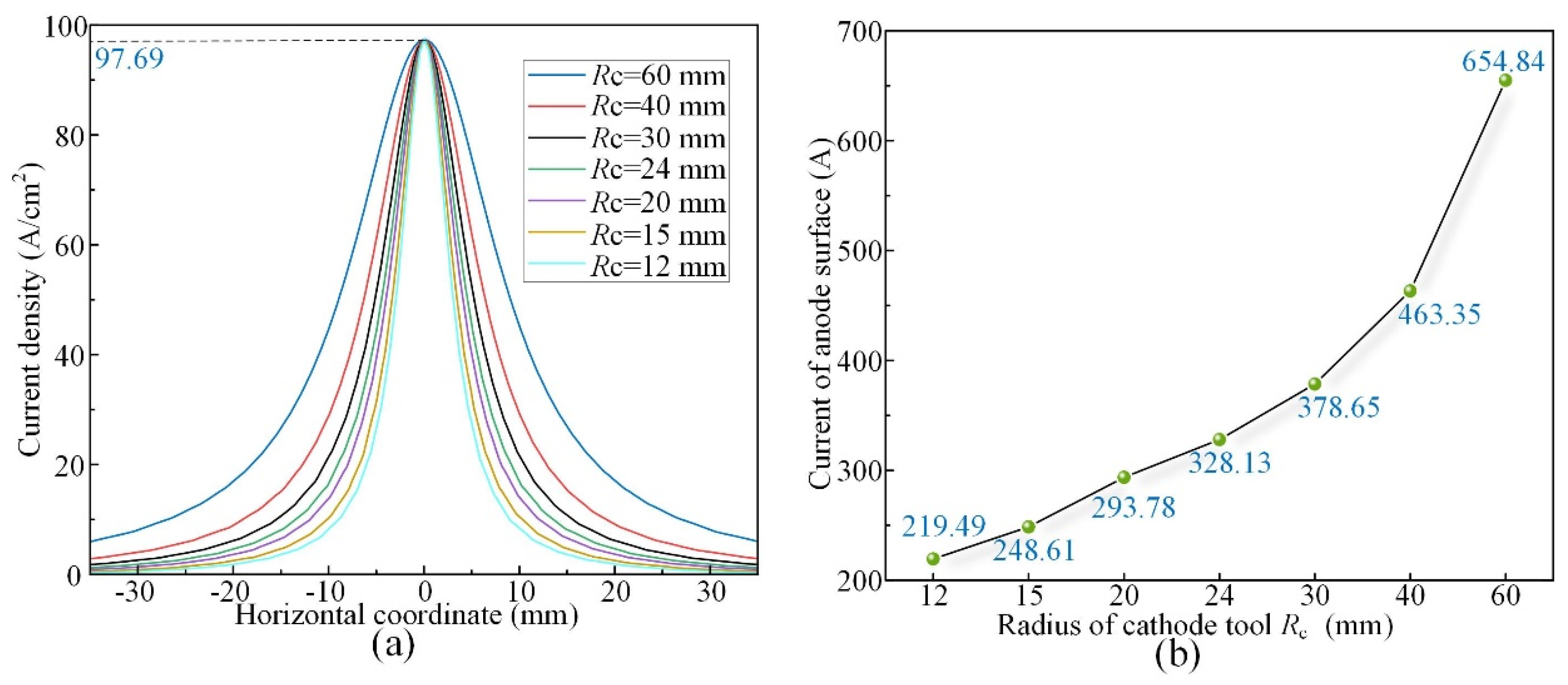
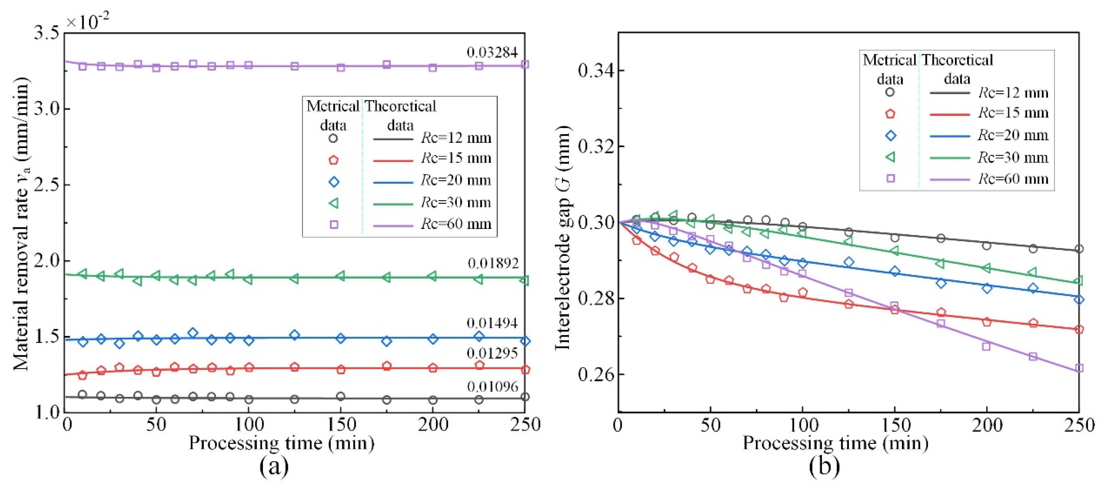
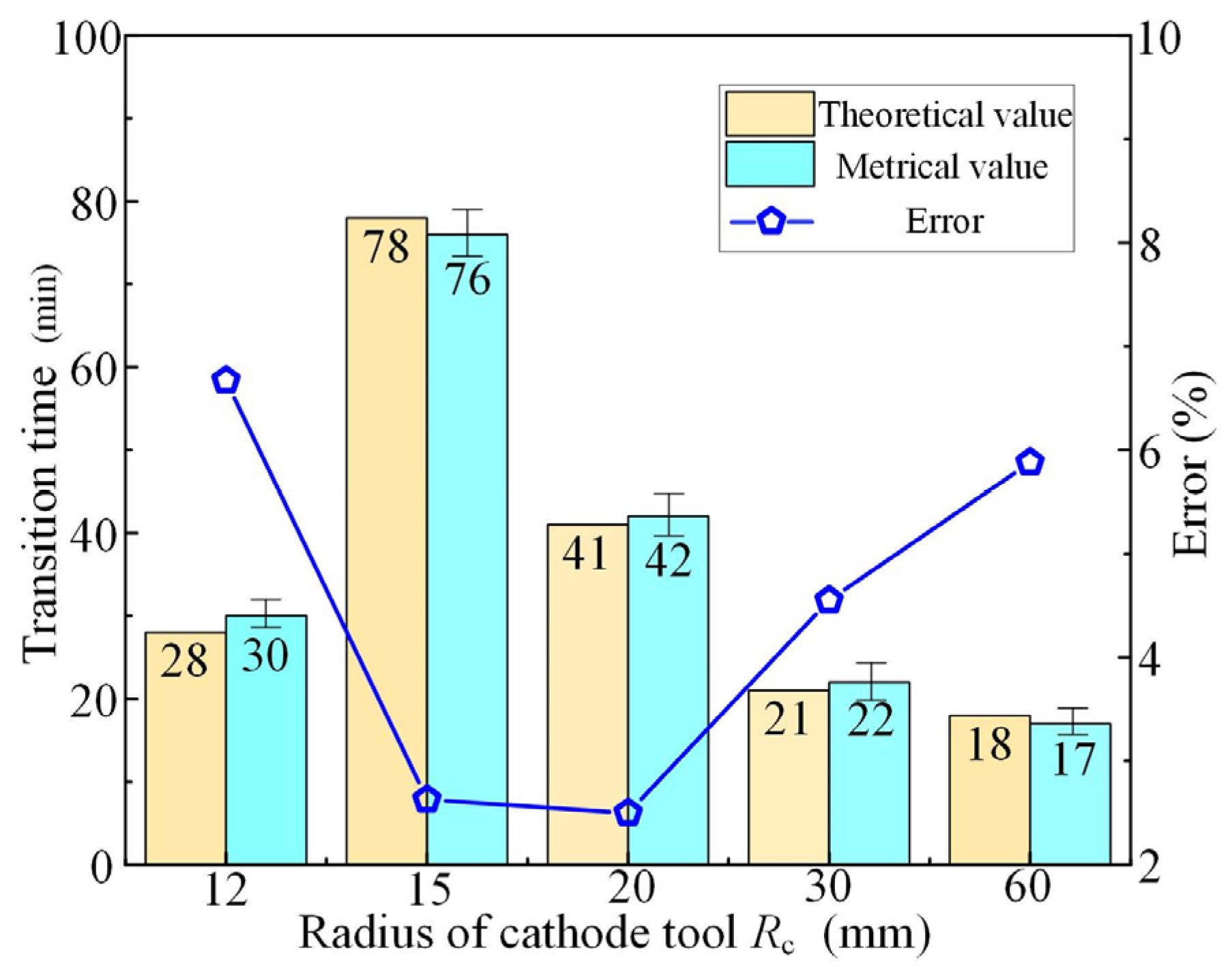
3.1. Effect of Cathode Tool Radii

In ICRECM, the cylindrical cathode works inside the annular anode, so the cathode radius is proportionally smaller than the anode radius. The radius formula between the cylindrical cathode and annular anode is
R c = R a n
where n is the angular speed ratio between the cylindrical cathode and annular anode.
A range of cathode radii (Rc = 12–60 mm) are selected to analyze the MRR and IEG. As shown in Figure 4a, the initial MRR increases with the increase in cathode radius. Over time, the final MRR is infinitely close to the feed rate (vf = 0.015 mm/min). The final MRR is slightly less than the feed rate for different cathode radii, which causes the IEG to gradually decrease. When the feed rate is greater than the initial MRR, the IEG will decrease rapidly to reach a quasi-equilibrium state. When the feed rate is less than the initial MRR, the machining slowly reaches a quasi-equilibrium state. In order to accurately calculate the transition time for processing to reach the quasi-equilibrium state, the following equation is obtained:
Δ v a = v f v a ( j ) < 10 4   mm / min
Figure 5 shows the transition time for different cathode radii. When Rc = 20 mm, the shortest transition time is only 41 min. When Rc = 30 mm, the MRR decreases to 0.015 mm/min at 139 min, and the IEG reaches the maximum of 0.41968 mm. When Rc = 60 mm, the quasi-equilibrium state is slowly reached at 227 min, and the IEG is as high as 0.84107 mm. Therefore, when the cathode radius exceeds 20 mm, the machining parameters need to be adjusted to reduce the transition time and IEG.
To explore the effect of the radius on the initial MRR, the current density of the anode surface is calculated for different cathode radii. It can be seen from Figure 6a that the peak current density of different cathode radii is the same. However, the area of high current density increases with the increase in the cathode radius. The current inside the anode workpiece is calculated by integrating the current density. As shown in Figure 6b, the initial current increases sharply with the increase in the cathode radius, which leads to the increase in the initial MRR.

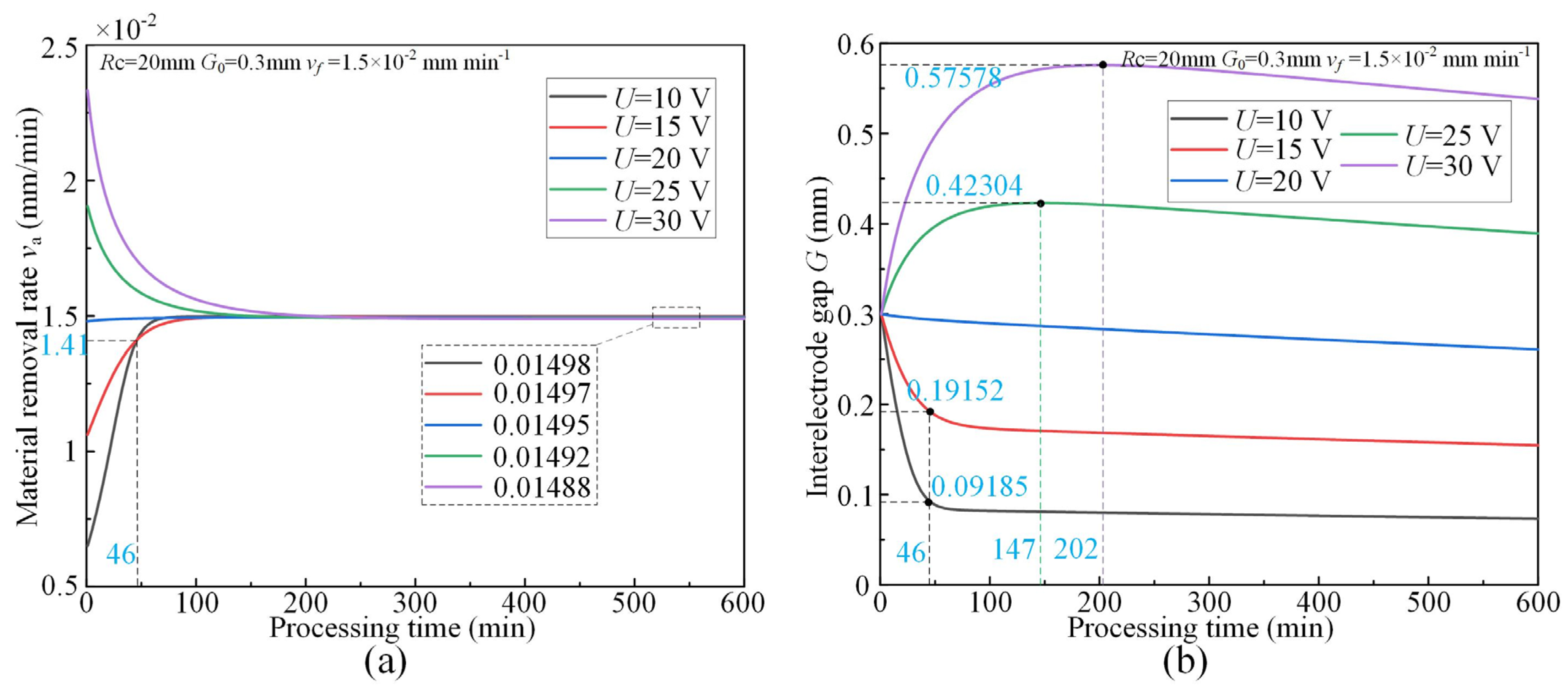
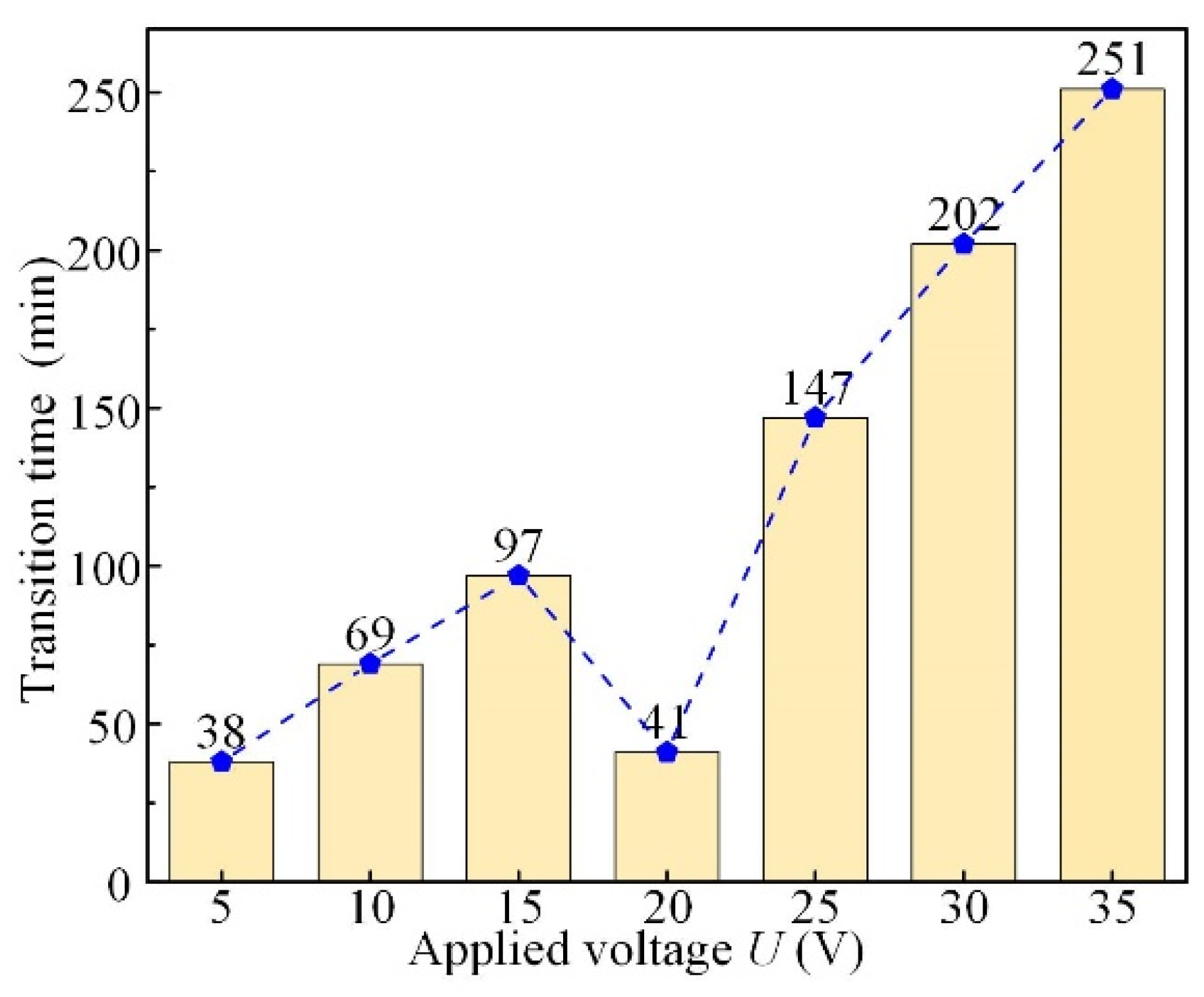
3.2. Effect of Applied Voltage

The applied voltage can determine the electric field strength, which strongly affects the MRR. Figure 7 shows the evolution of MRR and IEG over time for a series of applied voltages (U = 10–30 V). As shown in Figure 7a, MRRs are different at the initial time, but MRRs eventually tend to be consistent. When the machining is in a quasi-equilibrium state, the IEG increases with the increase in applied voltage, but the final MRR decreases slightly with the increase in applied voltage. After 46 min, the MRR of 10 V exceeds the MRR of 15 V to reach a quasi-equilibrium state earlier. The initial MRR of 10 V is very low, which causes the IEG to decrease rapidly from 0.3 mm to 0.09 mm. When the machining reaches a quasi-equilibrium state, the MRR with different applied voltages is slightly less than the feed rate (Figure 7a), which causes the IEG to gradually decrease with time (Figure 7b). When the voltage is greater than 20 V, IEG will have a peak value. The IEG reaches the peak value when the machining just reaches a quasi-equilibrium state. The peak values of IEG at 25 V and 30 V are 0.42304 mm and 0.57578 mm, respectively.
Figure 8 shows the transition time with different applied voltages. When U = 5 V, the transition time is shortest. However, the final IEG is far less than 0.1 mm, which cannot be realized in actual processing. When U = 20 V, the transition time is 41 min, and the IEG can be maintained to 0.27 mm. Therefore, the appropriate applied voltage will not only shorten the transition time but also maintain the IEG in the achievable range.

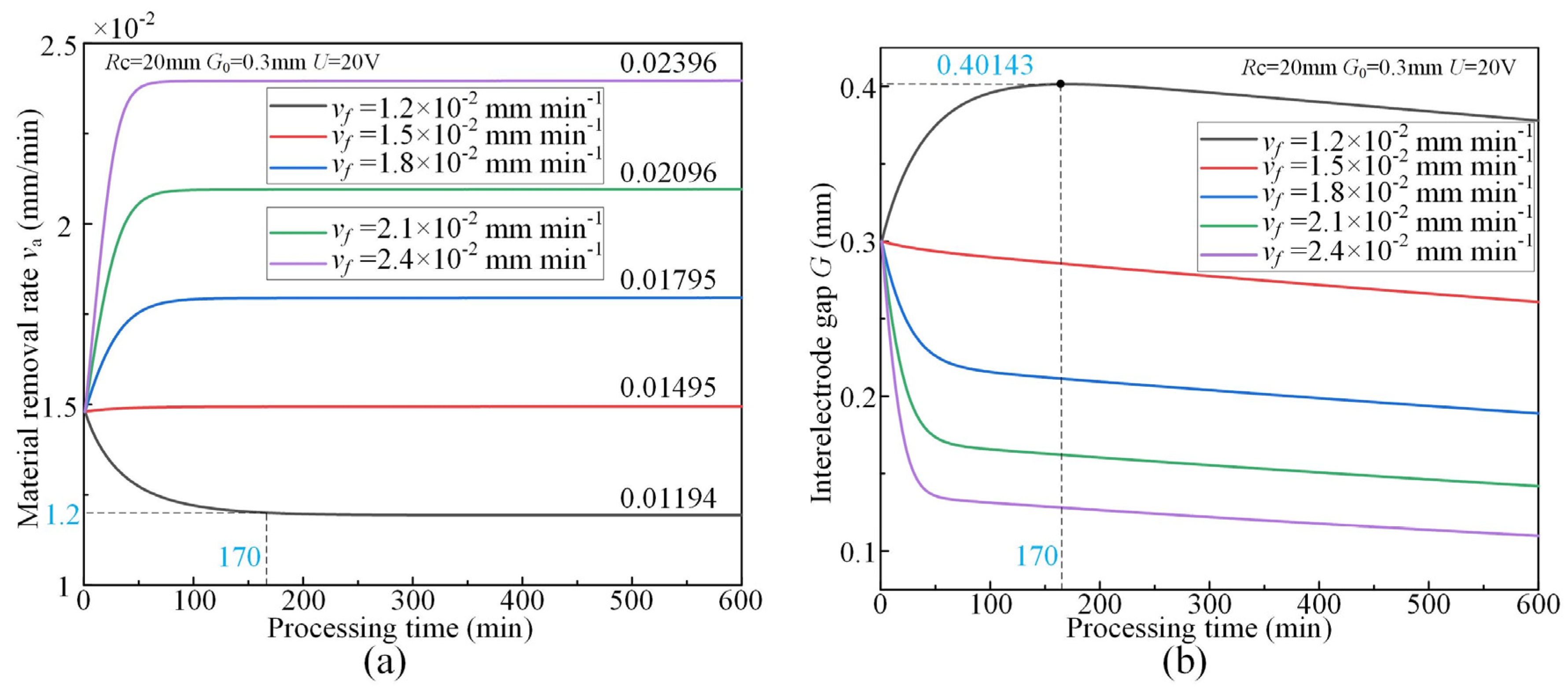
3.3. Effect of Feed Rate

A series of feed rates (vf = 0.012–0.024 mm/min) were selected to analyze the changes of MRR and IEG. It can be seen from Figure 9a that the final MRR is determined by the feed rate. It is different from conventional ECM in that the feed rate is always higher than the final MRR in ICRECM. This is due to the fact that the internal material of the anode gradually dissolves along the radius, and the internal radius gradually increases. When the machining is in a quasi-equilibrium state, the IEG decreases with the increase in the feed rate. Figure 10 shows the transition time for different feed rates. When vf = 0.015 mm/min, the transition time decreases to the minimum of 41 min. As the feed rate increases to more than 0.018 mm/min, the IEG changes sharply resulting in machining instability. When vf = 0.012 mm/min, it takes a long time to make the machining enter a quasi-equilibrium state. A suitable feed rate will make the IEG change smoothly, which is conducive to stable machining.

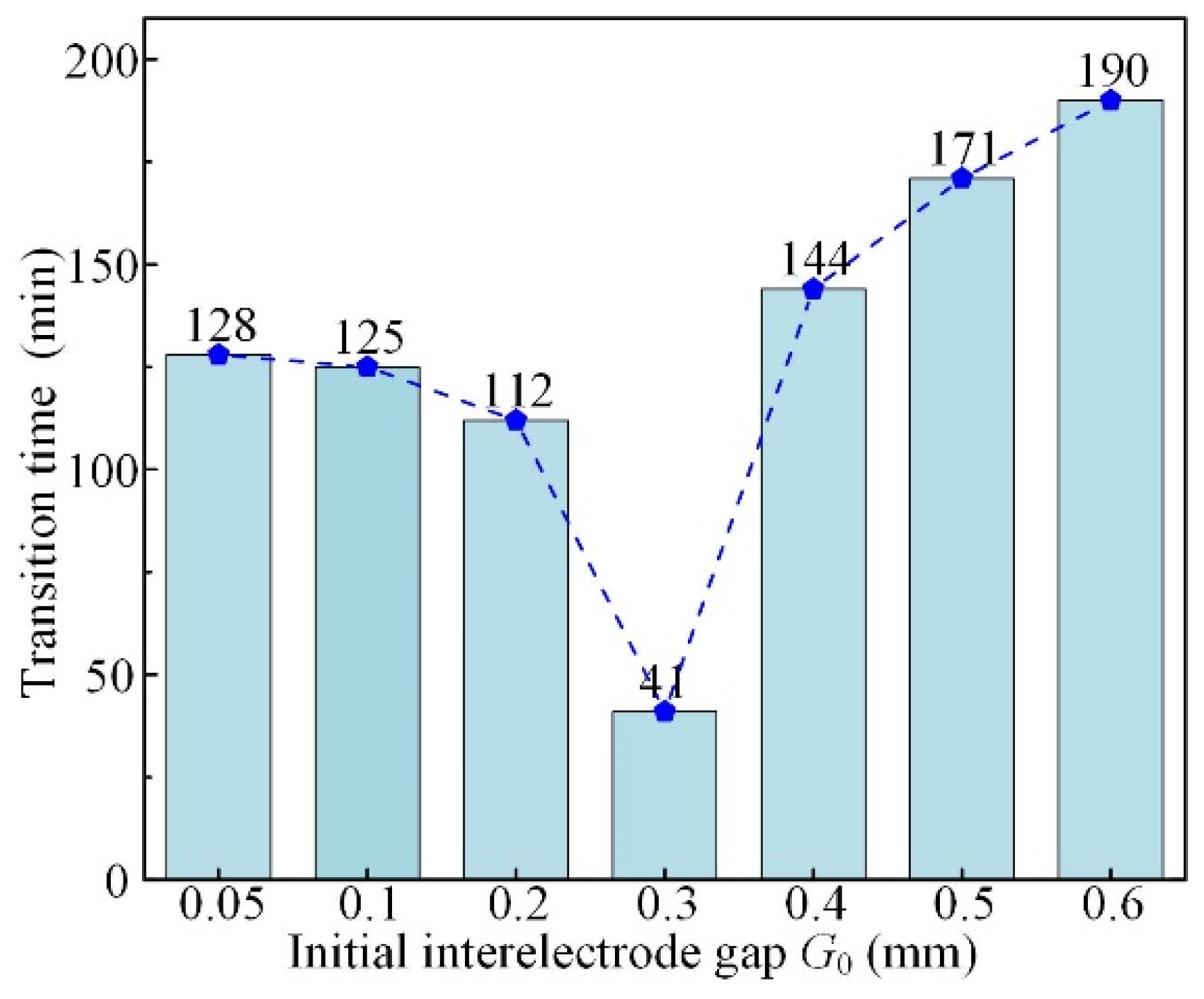
3.4. Effect of Initial Interelectrode Gap

Figure 11 shows the curves of MRR and IEG for different initial IEG (G0 = 0.1–0.5 mm). The curves of MRR and IEG with different initial IEG tend to be consistent, respectively, indicating that the initial IEG does not affect the final machining state. As shown in Figure 12, the initial IEG has a strong influence on the transition time. An appropriate initial IEG (G0 = 0.3 mm) can not only make the machining enter a quasi-equilibrium state quickly but also reduce the fluctuation of the machining gap, thereby improving the accuracy of electrochemical machining. When the machining reaches a quasi-equilibrium state, the IEG decreases slowly over time because the MRR is always slightly lower than the feed rate. This is quite different from conventional ECM in that the quasi-equilibrium state of ICRECM is accompanied by the gradual reduction in IEG.

4. Experimental Validation

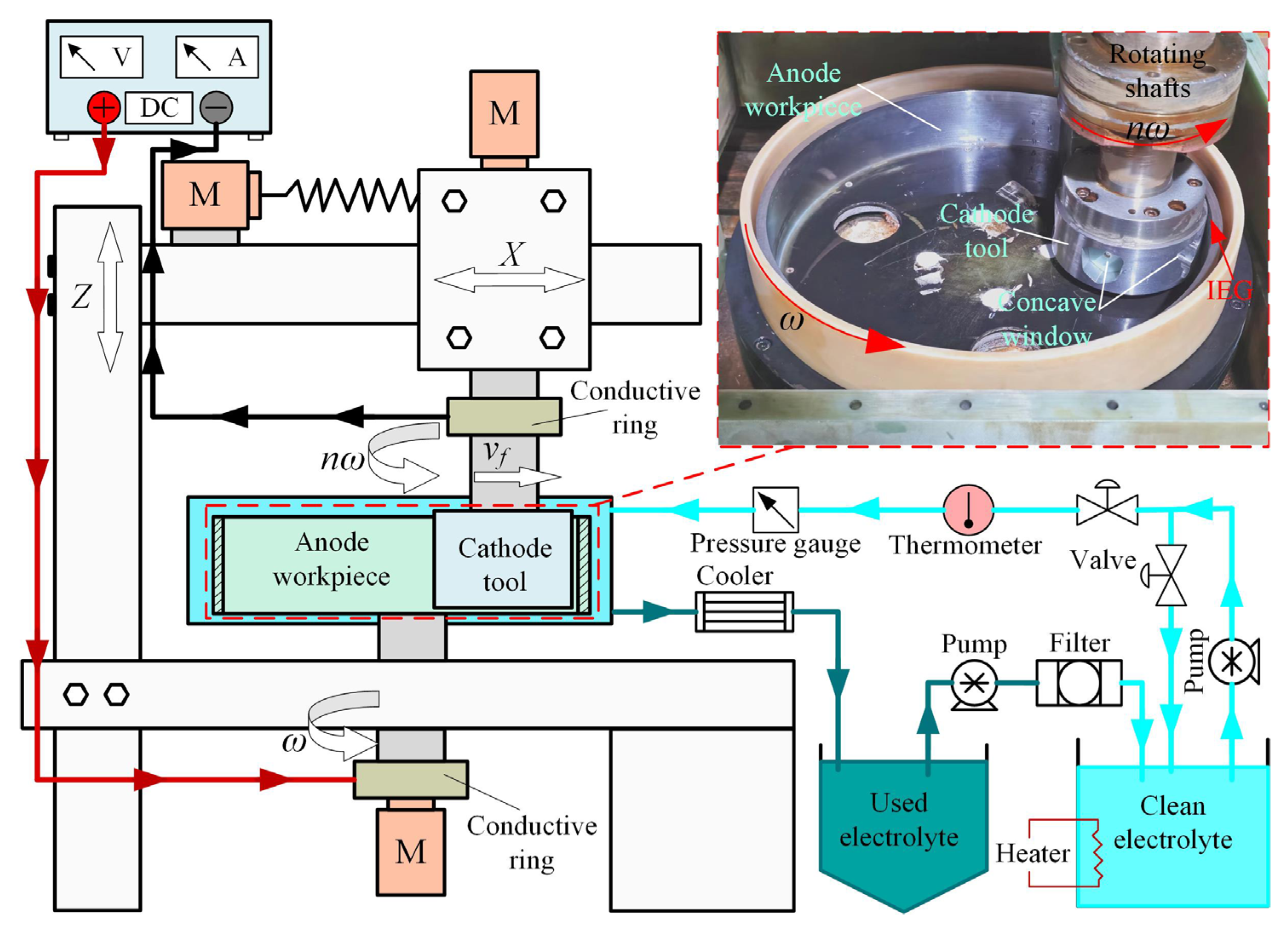
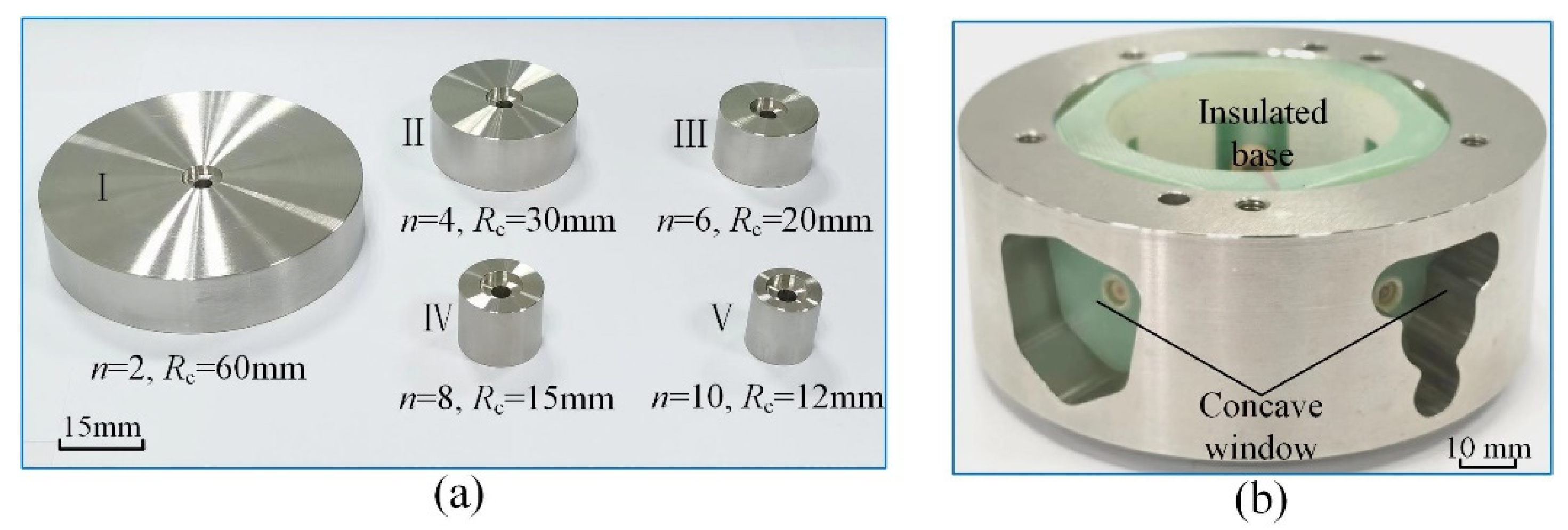
4.1. Experimental System

Figure 13 shows the developed experimental system for ICRECM, which consists of an electrode motion system, a power supply system and an electrolyte circulation system (electrolyte, cooler, heater and filter). The cylindrical cathode and annular anode were mounted on the upper and lower rotating shafts, respectively. The electrode motion system could realize the differential rotation of the workpiece and tool. The upper rotating shaft could realize feeding along the direction of the center line. The power supply system applied voltage to the rotating shafts through the conductive rings. The electrolyte circulation system enabled real-time filtration of electrolytic products and temperature control, so as to keep the electrolyte clean and temperature constant. The high-speed electrolyte with a constant temperature was pumped from jet nozzles and flows through the narrow electrode gap.
Table 1 summarizes the experimental parameters corresponding to the simulation parameters. Table 2 shows the detailed machining parameters of the comparative experiments. According to the initial MRR obtained from the simulation, the feed rates of groups 1 to 5 have been optimized to rapidly reach a quasi-equilibrium state. A variety of cathode tools were used for comparative experiments, which were made of 304 stainless steel. Cylindrical cathodes with different radii were selected for experiments of groups 1 to 5 (Figure 14a). A cylindrical cathode with concave windows was used for machining convex structures inside the annular part (Figure 14b), and it corresponded to the experimental parameters of the sixth group. To ensure the steadiness of the machining, the parameters of the sixth group were optimized so that there was almost no transition time.

4.2. Experimental Results

The experiments were conducted with the feed rate optimized according to the initial MRR obtained from the simulation. According to the geometry of the annular workpiece, the IEG could be obtained by the electrode motion system after each time interval (Δt). The material removal thickness could be obtained by measuring the thickness variation of the workpiece, and the MRR was obtained by dividing material removal thickness by the time interval. As shown in Figure 15, the MRR and IEG change smoothly by using the optimized feed rate, which is conducive to stable machining. The metrical data fluctuate slightly near the theoretical curves, indicating that the established model can predict well MRR and IEG during the machining. In order to better evaluate the established model, the proportional error between the theoretical data and metrical data can be computed as follows:
δ = r T r M r M × 100 %
where δ is the proportional error; rT is the theoretical value; rM is the metrical value.
Figure 16 shows the theoretical values and metrical values of the transition time, and the maximum error is 6.67%. The transition time can be shortened to 17 min with the optimized feed rate, so that the machining can quickly enter a quasi-equilibrium state. The experimental results show that the transition time is greatly shortened using the optimized feed rate.
Figure 17 shows the annular workpiece machined with the optimized feed rate (0.014 mm/min) and voltage (16 V). Clearly, a large amount of material was removed from the interior of the workpiece. The data on MRR and IEG with the optimum machining parameters are presented in Table 3. There is almost no fluctuation in MRR, indicating that the machining has reached a quasi-equilibrium state in a very short time. A short transition time can make the machining achieve higher precision. The metrical data are in good agreement with the theoretical data, which means that the established model can effectively predict the evolution process of MRR and IEG.

5. Conclusions

In this paper, the material removal process is simulated based on the established analysis model, which is verified by the developed experimental system. The following conclusions are summarized:
(1)
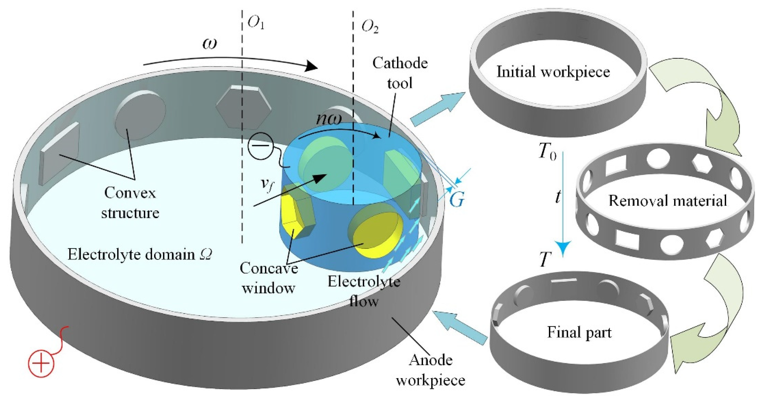
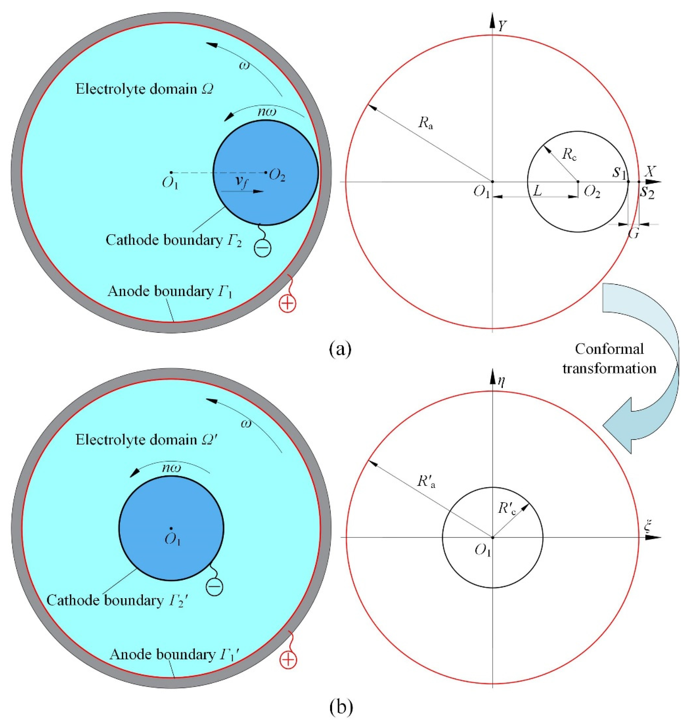
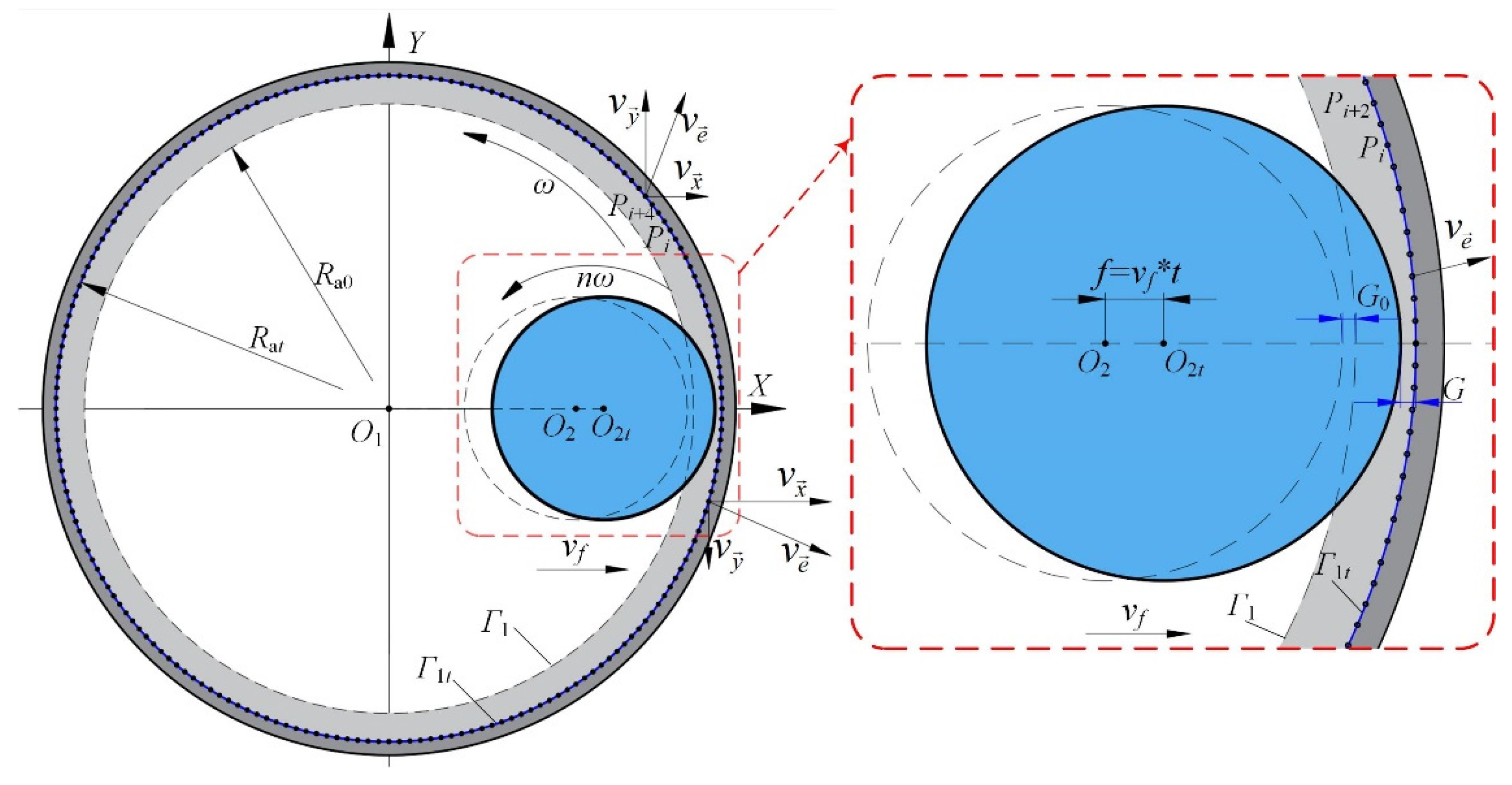
The complex electric field model of ICRECM is simplified by conformal transformation, and then the analytical solution of electric field intensity is exactly calculated. A material removal model is built on the basis of the electric field model, and the dynamic simulation of the material removal process is realized.
(2)
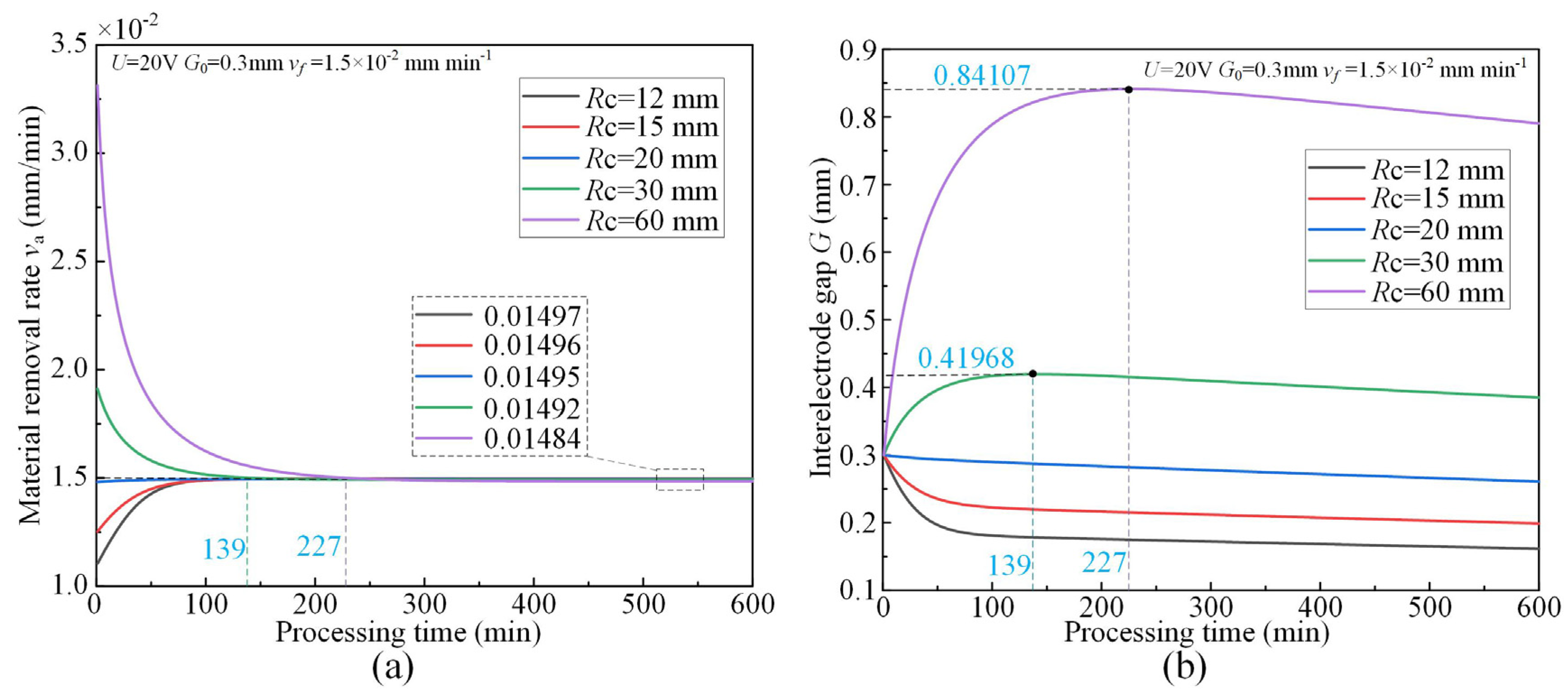
The simulative results indicate that the quasi-equilibrium state is accompanied by the gradual reduction in IEG. The initial MRR and final IEG increase with the increase in cathode radius. The MRR in the quasi-equilibrium state is determined by the feed rate. The initial IEG does not affect the final machining state, but it has a strong effect on the transition time.
(3)
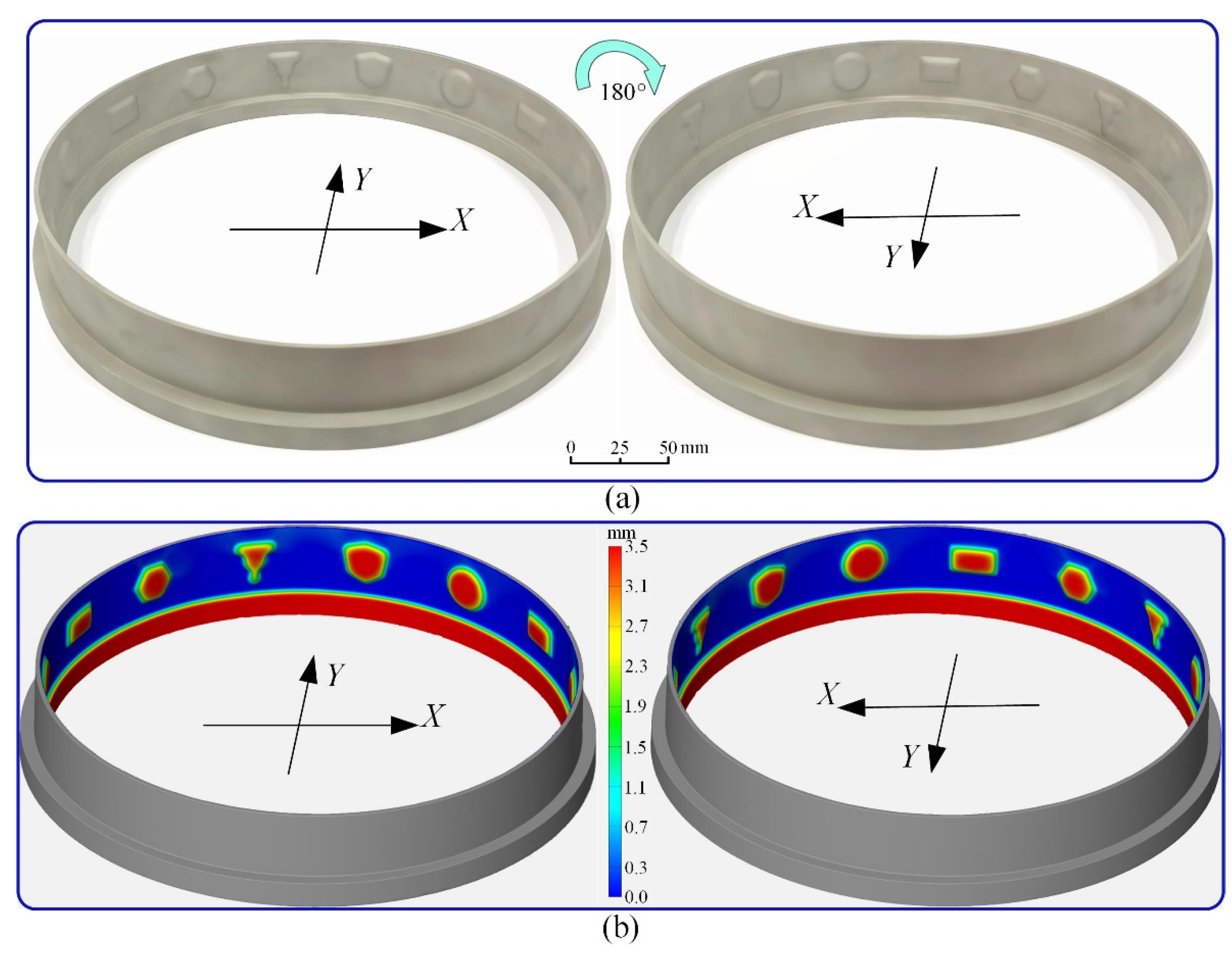
The experimental results show that the transition time can be greatly shortened using the optimized feed rate (Minimum transition time 17 min). The convex structures are successfully machined inside the annular workpiece with the optimized feed rate (0.014 mm/min) and voltage (16 V). There is almost no fluctuation in MRR during the manufacturing of convex structures, indicating that the machining has reached a quasi-equilibrium state in a very short time.
(4)
There are optimum parameters to make the machining enter the quasi-equilibrium state at the beginning. The metrical data are in good agreement with the theoretical data (Maximum error 1.975%), indicating that the established model can effectively predict the evolution process of MRR and IEG.

Author Contributions

Conceptualization, D.Z.; Methodology, S.Z.; Software, T.F.; Investigation, S.Z. and T.F.; Data curation, S.Z. and T.F.; Writing—original draft, S.Z.; Writing—review & editing, D.W. and D.Z.; Supervision, D.W.; Funding acquisition, D.W. and D.Z. All authors have read and agreed to the published version of the manuscript.

Funding

This research was funded by the National Natural Science Foundation of China [grant number 52175414], National Natural Science Foundation of China for Creative Research Groups [grant number 51921003], and Natural Science Foundation of Jiangsu Province of China [grant number BK20220134].

Data Availability Statement

All data generated or analyzed during this study are included in this article.

Conflicts of Interest

The authors declare no conflict of interest.

References

  1. Xu, Z.Y.; Xu, Q.; Zhu, D.; Gong, T. A high efficiency electrochemical machining method of blisk channels. CIRP Ann. 2013, 62, 187–190. [Google Scholar] [CrossRef]
  2. Klocke, F.; Zeis, M.; Klink, A.; Veselovac, D. Experimental Research on the Electrochemical Machining of Modern Titanium- and Nickel-based Alloys for Aero Engine Components. Procedia CIRP 2013, 6, 368–372. [Google Scholar] [CrossRef]
  3. Poursaeidi, E.; Kavandi, A.; Vaezi, K.; Kalbasi, M.R.; Mohammadi Arhani, M.R. Fatigue crack growth prediction in a gas turbine casing. Eng. Fail. Anal. 2014, 44, 371–381. [Google Scholar] [CrossRef]
  4. Wang, D.; Yu, J.; Le, H.; Zhu, D. Localized sinking electrochemical machining of pre-shaped convex structure on revolution surface using specifically designed cathode tool. J. Manuf. Process. 2023, 99, 605–617. [Google Scholar] [CrossRef]
  5. Scippa, A.; Grossi, N.; Campatelli, G. FEM based Cutting Velocity Selection for Thin Walled Part Machining. Procedia CIRP 2014, 14, 287–292. [Google Scholar] [CrossRef]
  6. Kundu, P.; Luo, X.; Qin, Y.; Chang, W.; Kumar, A. A novel current sensor indicator enabled WAFTR model for tool wear prediction under variable operating conditions. J. Manuf. Process. 2022, 82, 777–791. [Google Scholar] [CrossRef]
  7. Bolsunovskiy, S.; Vermel, V.; Gubanov, G.; Kacharava, I.; Kudryashov, A. Thin-walled part machining process parameters optimization based on finite-element modeling of workpiece vibrations. Procedia CIRP 2013, 8, 276–280. [Google Scholar] [CrossRef]
  8. Zadafiya, K.; Kumari, S.; Chattarjee, S.; Abhishek, K. Recent trends in non-traditional machining of shape memory alloys (SMAs): A review. CIRP J. Manuf. Sci. Technol. 2021, 32, 217–227. [Google Scholar] [CrossRef]
  9. Singh Patel, D.; Agrawal, V.; Ramkumar, J.; Jain, V.K.; Singh, G. Micro-texturing on free-form surfaces using flexible-electrode through-mask electrochemical micromachining. J. Mater. Process. Technol. 2020, 282, 116644. [Google Scholar] [CrossRef]
  10. Thangamani, G.; Thangaraj, M.; Moiduddin, K.; Mian, S.H.; Alkhalefah, H.; Umer, U. Performance Analysis of Electrochemical Micro Machining of Titanium (Ti-6Al-4V) Alloy under Different Electrolytes Concentrations. Metals 2021, 11, 247. [Google Scholar] [CrossRef]
  11. Hotoiu, L.; Deconinck, J.; Diver, C.; Tormey, D. Ultra-short pulse simulation for characterising oxide layer formation on stainless steel during μECM. CIRP J. Manuf. Sci. Technol. 2020, 31, 370–376. [Google Scholar] [CrossRef]
  12. Liu, J.; Duan, S.; Zhou, Q.; Xu, Z. Optimization of tool nozzle structure for electrochemical boring of inner cavity in engine spindles. CIRP J. Manuf. Sci. Technol. 2023, 44, 1–15. [Google Scholar] [CrossRef]
  13. Rajurkar, K.P.; Sundaram, M.M.; Malshe, A.P. Review of Electrochemical and Electrodischarge Machining. Procedia CIRP 2013, 6, 13–26. [Google Scholar] [CrossRef]
  14. Sharma, V.; Patel, D.S.; Jain, V.K.; Ramkumar, J. Wire electrochemical micromachining: An overview. Int. J. Mach. Tools Manuf. 2020, 155, 103579. [Google Scholar] [CrossRef]
  15. Zhang, J.; Wang, D.; Le, H.; Fu, T.; Zhu, D. Effect of carbides on the electrochemical dissolution behavior of solid-solution strengthened cobalt-based superalloy Haynes 188 in NaNO3 solution. Corros. Sci. 2023, 220, 111270. [Google Scholar] [CrossRef]
  16. Wang, D.; He, B.; Zhu, Z.; Zhu, D. Investigation of the Material Removal Process in Counter-rotating Electrochemical Machining. Procedia CIRP 2018, 68, 704–708. [Google Scholar] [CrossRef]
  17. De Silva, A.K.M.; Altena, H.S.J.; McGeough, J.A. Influence of electrolyte concentration on copying accuracy of precision-ECM. CIRP Ann.—Manuf. Technol. 2003, 52, 165–168. [Google Scholar] [CrossRef]
  18. Béjar, M.A.; Gutiérrez, F. On the determination of current efficiency in electrochemical machining with a variable gap. J. Mater. Process. Technol. 1993, 37, 691–699. [Google Scholar] [CrossRef]
  19. Clifton, D.; Mount, A.R.; Alder, G.M.; Jardine, D. Ultrasonic measurement of the inter-electrode gap in electrochemical machining. Int. J. Mach. Tools Manuf. 2002, 42, 1259–1267. [Google Scholar] [CrossRef]
  20. Hewidy, M.S.; Ebeid, S.J.; El-Taweel, T.A.; Youssef, A.H. Modelling the performance of ECM assisted by low frequency vibrations. J. Mater. Process. Technol. 2007, 189, 466–472. [Google Scholar] [CrossRef]
  21. Hewidy, M.S. Controlling of metal removal thickness in ECM process. J. Mater. Process. Technol. 2005, 160, 348–353. [Google Scholar] [CrossRef]
  22. Lu, Y.; Liu, K.; Zhao, D. Experimental investigation on monitoring interelectrode gap of ECM with six-axis force sensor. Int. J. Adv. Manuf. Technol. 2011, 55, 565–572. [Google Scholar] [CrossRef]
  23. Rajurkar, K.P.; Wei, B.; Kozak, J.; McGeough, J.A. Modelling and Monitoring Interelectrode Gap in Pulse Electrochemical Machining. CIRP Ann. 1995, 44, 177–180. [Google Scholar] [CrossRef]
  24. Mount, A.R.; Clifton, D.; Howarth, P.; Sherlock, A. An integrated strategy for materials characterisation and process simulation in electrochemical machining. J. Mater. Process. Technol. 2003, 138, 449–454. [Google Scholar] [CrossRef]
  25. Wang, D.; Li, J.; He, B.; Zhu, D. Analysis and control of inter-electrode gap during leveling process in counter-rotating electrochemical machining. Chin. J. Aeronaut. 2019, 32, 2557–2565. [Google Scholar] [CrossRef]
  26. Cao, W.; Wang, D.; Zhu, D. Modeling and experimental validation of interelectrode gap in counter-rotating electrochemical machining. Int. J. Mech. Sci. 2020, 187, 105920. [Google Scholar] [CrossRef]
  27. Chen, Y.; Zhou, X.; Chen, P.; Wang, Z. Electrochemical machining gap prediction with multi-physics coupling model based on two-phase turbulence flow. Chin. J. Aeronaut. 2020, 33, 1057–1063. [Google Scholar] [CrossRef]
  28. Grafov, B.M. The general approach to the theory of the first passage problem for electrochemical stochastic diffusion in equilibrium. Russ. J. Electrochem. 2017, 53, 897–902. [Google Scholar] [CrossRef]
  29. Wang, Y.; Xu, Z.; Meng, D.; Liu, L.; Fang, Z. Multi-Physical Field Coupling Simulation and Experiments with Pulse Electrochemical Machining of Large Size TiAl Intermetallic Blade. Metals 2023, 13, 985. [Google Scholar] [CrossRef]
  30. Wang, D.; Zhu, Z.; Zhu, D.; He, B.; Ge, Y. Reduction of stray currents in counter-rotating electrochemical machining by using a flexible auxiliary electrode mechanism. J. Mater. Process. Technol. 2017, 239, 66–74. [Google Scholar] [CrossRef]
  31. Cao, W.; Wang, D.; Cui, G.; Le, H. Analysis of the roundness error elimination in counter-rotating electrochemical machining. J. Manuf. Process. 2022, 76, 57–66. [Google Scholar] [CrossRef]
  32. Zhou, S.; Wang, D.; Cao, W.; Zhu, D. Investigation of anode shaping process during co-rotating electrochemical machining of convex structure on inner surface. Chin. J. Aeronaut. 2022. [CrossRef]
  33. Islam, S.M.R.; Akbulut, A.; Arafat, S.M.Y. Exact solutions of the different dimensional CBS equations in mathematical physics. Partial Differ. Equ. Appl. Math. 2022, 5, 100320. [Google Scholar] [CrossRef]
  34. Galeriu, C. Electric charge in hyperbolic motion: The special conformal transformation solution. Eur. J. Phys. 2019, 40, 065203. [Google Scholar] [CrossRef]
  35. Chantry, L.; Cayatte, V.; Sauty, C. Conformal representation of Kerr space-time poloidal sub-manifolds. Class. Quantum Gravity 2020, 37, 105003. [Google Scholar] [CrossRef]
  36. Wang, Z.G.; Liao, T.; Wang, Y.N. Modeling electric field of power metal-oxide-semiconductor field-effect transistor with dielectric trench based on Schwarz-Christoffel transformation. Chin. Phys. B 2019, 28, 058503. [Google Scholar] [CrossRef]
  37. Eyal, O.; Goldstein, A. Gauss’ law for moving charges from first principles. Results Phys. 2019, 14, 102454. [Google Scholar] [CrossRef]
  38. Bermúdez Manjarres, A.D.; Nowakowski, M.; Batic, D. Coulomb law in the nonuniform Euler-Heisenberg theory. Int. J. Mod. Phys. A 2020, 35, 2050211. [Google Scholar] [CrossRef]
  39. Gow, R.; McGuire, G. Invariant rational functions, linear fractional transformations and irreducible polynomials over finite fields. Finite Fields Their Appl. 2022, 79, 101991. [Google Scholar] [CrossRef]
  40. Ter Horst, S. A pre-order on operators with positive real part and its invariance under linear fractional transformations. J. Math. Anal. Appl. 2014, 420, 1376–1390. [Google Scholar] [CrossRef]
  41. Jain, V.K.; Gehlot, D. Anode shape prediction in through-mask-ECMM using FEM. Mach. Sci. Technol. 2015, 19, 286–312. [Google Scholar] [CrossRef]
  42. Pattavanitch, J.; Hinduja, S.; Atkinson, J. Modelling of the electrochemical machining process by the boundary element method. CIRP Ann.—Manuf. Technol. 2010, 59, 243–246. [Google Scholar] [CrossRef]
  43. Jia, X. Electric potential and electric field between two confocal parabolic conductor plates. J. Zhejiang Univ. Sci. Ed. 2018, 45, 427–428. [Google Scholar]
  44. Mithu, M.A.H.; Fantoni, G.; Ciampi, J.; Santochi, M. On how tool geometry, applied frequency and machining parameters influence electrochemical microdrilling. CIRP J. Manuf. Sci. Technol. 2012, 5, 202–213. [Google Scholar] [CrossRef]
  45. Cao, W.; Wang, D.; Ren, Z.; Zhu, D. Evolution of convex structure during counter-rotating electrochemical machining based on kinematic modeling. Chin. J. Aeronaut. 2021, 34, 39–49. [Google Scholar] [CrossRef]
Figure 1. The principle of ICRECM.
Metals 13 01771 g001
Figure 2. Conformal transformation of electric field model (a) original model; (b) equivalent model.
Metals 13 01771 g002
Figure 3. Schematic of the dynamic material removal for ICRECM.
Metals 13 01771 g003
Figure 4. Variation of material removal rate and interelectrode gap for different cathode radii (a) material removal rate; (b) interelectrode gap.
Metals 13 01771 g004
Figure 5. Variation of transition time with different cathode radii.
Metals 13 01771 g005
Figure 6. Current of anode surface for various cathode radii (a) current density on anode surface; (b) current on anode surface.
Metals 13 01771 g006
Figure 7. Variation of material removal rate and interelectrode gap for different applied voltages (a) material removal rate; (b) interelectrode gap.
Metals 13 01771 g007
Figure 8. Variation of transition time with different applied voltages.
Metals 13 01771 g008
Figure 9. Variation of material removal rate and interelectrode gap for different feed rates (a) material removal rate; (b) interelectrode gap.
Metals 13 01771 g009
Figure 10. Variation in transition time with different feed rates.
Metals 13 01771 g010
Figure 11. Variation of material removal rate and interelectrode gap for different initial interelectrode gaps (a) material removal rate; (b) interelectrode gap.
Metals 13 01771 g011
Figure 12. Variation of transition time with different initial interelectrode gaps.
Metals 13 01771 g012
Figure 13. Schematic of the experimental system.
Metals 13 01771 g013
Figure 14. Photographs of various cathodes (a) the cylindrical cathodes; (b) the cathode tool with concave windows.
Metals 13 01771 g014
Figure 15. Comparison of metrical and theoretical data (a) material removal rate; (b) interelectrode gap.
Metals 13 01771 g015
Figure 16. Transition time of different parameters.
Metals 13 01771 g016
Figure 17. Workpiece processed by cathode tool with concave windows (a) photographs of the processed workpiece; (b) workpiece measured by GOM Scan.
Metals 13 01771 g017
Table 1. Machining conditions.
ParametersValue
Electrolyte conditions30 °C 0.5 Mpa
Electrolyte type20% NaNO3
Anode material304 SS
Applied voltage, U (V)16, 20
Initial IEG, G0 (mm) 0.3
Radius of the anode, Ra (mm)120, 150
Angular speed of anode, ω (r/min)2
Processing time (min) 250
Table 2. Parameters of comparative experiments.
Machining ParameterValue
123456
Radius of the cathode, Rc (mm)121520306050
Radius of the anode, Ra (mm)120120120120120150
Angular velocity ratio, n1086423
Feed rate, vf (mm/min)0.0110.0130.0150.0190.0330.014
Applied voltage, U (V)202020202016
Table 3. Comparison of metrical and theoretical data for optimum machining parameters.
Processing Time (min)MRR (mm/min)IEG (mm)
Metrical DataTheoretical DataError (%)Metrical DataTheoretical DataError (%)
100.013690.013861.2420.30090.29860.764
200.013820.013890.5070.29890.29740.502
300.013740.013911.2370.29760.29640.403
400.013840.013920.5780.29640.29550.304
500.013890.013930.2880.29550.29470.271
600.013850.013930.5780.29430.2940.102
700.013670.013941.9750.29310.29330.068
800.013920.013940.1720.29230.29270.137
900.013860.013940.5770.29150.29220.24
1000.013720.013951.6760.29090.29160.241
1250.013850.013950.7220.28940.29030.311
1500.013990.013950.2860.28850.2890.173
1750.013880.013960.5980.28740.28780.139
2000.013920.013960.2870.28690.28660.105
2250.013890.013960.5040.2860.28530.245
2500.013910.013960.3590.28470.28420.176
Disclaimer/Publisher’s Note: The statements, opinions and data contained in all publications are solely those of the individual author(s) and contributor(s) and not of MDPI and/or the editor(s). MDPI and/or the editor(s) disclaim responsibility for any injury to people or property resulting from any ideas, methods, instructions or products referred to in the content.

