Abstract
A two-dimensional transient inverse heat-conduction problem (2DIHCP) was established to determine the mold heat flux using observed temperatures. The sequential regularization method (SRM) was used with zeroth-, first-, and second-order spatial regularization to solve the 2DIHCP. The accuracy of the 2DIHCP was investigated under two strict test conditions (Case 1: heat flux with time-spatial periodically varying, and Case 2: that with sharp variations). The effects of the number of future time steps, regularization parameters, order of regularization, discrete grids, and time step size on the accuracy of the 2DIHCP were analyzed. The results showed that the minimum relative error (epred) of the predicted Case 1 heat flux is 5.05%, 5.39%, and 5.88% for zeroth-, first-, and second-order spatial regularization, respectively. The corresponding values for the predicted Case 2 heat flux are 6.31%, 6.30%, and 6.36%. Notably, zeroth- and first-order spatial regularization had higher accuracy than second-order spatial regularization, while zeroth-order spatial regularization was comparable to first-order. Additionally, first-order spatial regularization was more accurate in reconstructing heat flux containing sharp spatial variations. The CPU time of the predicted Case 2 heat flux is 1.71, 1.71, and 1.70 s for zeroth-, first-, and second-order spatial regularization, respectively. The corresponding values for the predicted Case 1 heat flux are 6.18, 6.15, and 6.17 s. It is noteworthy that the choice of spatial regularization order does not significantly impact the required computing time. Lastly, the minimum epred of Case 2 heat flux with zeroth-order spatial regularization is 7.96%, 6.42%, and 7.87% for time step sizes of 1/fs, 1/2fs, and 1/5fs, respectively. The accuracy of the inverse analysis displays an initial improvement followed by degradation as the time step size decreases. A recommended time step size is 1/2fs, where fs denotes the temperature-sampling rate.
1. Introduction
Many surface defects found in the final rolled product can often be traced back to heat transfer in the continuous casting mold during the early stages of molten steel solidification [1,2,3]. The mold heat flux, especially at the mold meniscus area, is highly complex due to the transient nature of the infiltration of lubricant liquid mold flux, intense fluid flow, and mold oscillation. This complexity poses a significant challenge in obtaining a clear and comprehensive understanding of all the dynamics within the system. Fluctuations in the mold heat flux reflect the solidification processes within the mold, and precise measurement of the mold heat flux is crucial to ensuring the quality of the continuous casting slab [2,4,5,6,7,8,9].
Modern software makes calculating the mold temperature field by solving the Fourier heat transfer partial differential equation (PDE) with given initial and boundary conditions easy. However, accurately determining the boundary conditions, such as the mold heat flux, can be difficult and often requires estimation from measured temperatures. The measured temperatures cannot be used to directly measure heat flux at the meniscus due to the transient temperature field in the copper mold, especially at the mold meniscus area, where significant heat flows longitudinally upward to the cold top of the mold.
Mathematically, the calculation of heat flux from observed temperatures is a common inverse problem that involves finding the heat flux with the highest probability of minimizing the difference between the calculated temperatures T and the observed temperatures Y [10,11,12]. This type of inverse heat-conduction problem can be seen as an optimization problem with Fourier heat transfer partial differential equation constraints [13]. Nevertheless, inverse problems are often categorized as ill-posed problems, which means that there may not exist a solution or the solution may not be unique. As a result, stabilization techniques are necessary to obtain reliable results for the inverse problem [13].
Stabilization techniques for inverse problems have two main categories: gradient-based methods and stochastic-based methods. Gradient-based methods include the Levenberg–Marquardt method [12,14,15,16], the function specification method [17], and the conjugate gradient method [18,19,20]. Stochastic-based methods encompass the Bayesian method [21], the fuzzy inference method [22], and the deep neural network algorithms [23]. Additionally, for transient heat transfer phenomena, the choice of time domain for utilizing measurements plays a crucial role in classifying the solution method. There are three proposed time domains: (1) only to the present time, (2) to the present time plus a few future time steps, and (3) the complete time domain. Methods based on the time domains (1) and (2) are sequential. Methods based on time domains (1) and (2) are sequential. The first method, using measurements only up to the present time (1), is often referred to as the Stolz method. In the second method (2), a few future temperatures are considered, originally proposed by Beck [11], and the associated algorithms are termed sequential. However, sequential methods based on time domains (1) and (2) tend to become unstable when small-time steps are used in the analysis. On the other hand, the whole-time domain approach (3) is powerful because it allows for very small-time steps, but it may not be as computationally efficient. Most stabilization techniques, such as function specification and regularization methods, can be applied in both sequential and whole-domain estimation forms [18,19,20,24].
In the continuous casting research community, Brimacomb et al. [25] employed the whole-domain zeroth-order regularization method to estimate mold heat flux under two-dimensional steady-state thermal conditions. Thomas et al. [26] introduced an inverse heat-conduction problem aimed at extracting insights into heat transfer at the meniscus based on thermocouple measurements. This model facilitates a deeper understanding of heat transfer dynamics at the meniscus during continuous steel casting. Yao and Wang et al. [27,28,29,30] developed a two-dimensional transient inverse heat transfer problem for calculating secondary cooling heat transfer using a nonlinear estimation approach. This inverse problem-based analysis enhances comprehension of nonuniform heat transfer in continuous round billet casting by enabling the identification of the unknown thermal resistance between the billet and the mold. Goldschmit et al. [31,32] devised an inverse analysis model employing regularization techniques to assess mold heat fluxes based on temperatures recorded by thermocouples embedded in the mold wall. Talukdar et al. [33] formulated a steady inverse heat-conduction model utilizing the conjugate gradient method to ascertain the heat flux across the surface of a continuous casting mold from observed temperatures. Wang et al. [19] developed a two-dimensional transient inverse heat-conduction problem using the whole-time domain conjugate gradient method to estimate the mold heat flux. Jayakrishna et al. [34] pioneered a three-dimensional steady-state inverse heat-conduction problem for parameter estimation, aiming to capture the mold heat flux. Indeed, Beck’s sequential function specification method has gained widespread acceptance and demonstrated its effectiveness in resolving one-dimensional inverse heat-conduction problems aimed at determining the heat flux of continuous casting mold [35,36]. This method operates on the assumption that the heat flux remains constant or follows a linear function over a specified number of future time steps. By selecting an appropriate number of future time steps, the stability of the solution in the time domain can be enhanced [27,37]. However, the sequential function specification method tends to exhibit instability when small-time steps are employed in the inverse analysis, particularly when reconstructing heat flux for two- and three-dimensional heat transfer problems with spatiotemporal variations [38,39,40].
Precisely online, determining the mold heat flux remains a focal point of research and presents a substantial challenge [41,42,43,44]. The heat flux in the mold exhibits variations in both the vertical and horizontal directions across the mold surface [24,45,46,47]. Monitoring the temperature of the continuous casting mold typically involves the use of numerous thermal sensors, such as thermocouples and fiber-optic temperature sensors [48]. Advances in continuous casting technology have given rise to fast mold thermal monitoring systems with temperature-sampling rates exceeding 10 Hz. These systems offer more detailed insights into mold breakout, the infiltration of liquid mold flux into the mold/shell gap, and the solidification behavior of liquid steel [49,50]. Subsequently, the requirements for addressing the inverse problem of online reconstructing mold heat flux using observed temperatures can be summarized as follows: ensuring the numerical solution’s stability, achieving rapid heat flux reconstruction, and effectively handling the discontinuous functional form of the unknown. Initially, the sequential method is considered more suitable than the whole-time domain approach due to the latter’s inherent feedback time delay during heat flux calculation. However, it is worth noting that the increased temperature-sampling rate resulting from the small-time step in the sequential method may lead to reduced accuracy in heat flux reconstruction [11,38]. Moreover, the functional form of the known boundary heat flux may exhibit discontinuities. Fachinotti et al. [51] have emphasized that regularization methods enable accurate capture of jump discontinuities within the unknown function.
The aim of this study is to establish a two-dimensional transient inverse heat-conduction problem (2DIHCP) using the sequential regularization method (SRM) to determine the mold heat flux from temperature data. This method introduces spatial regularizations to enhance the sequential approach [51,52,53,54]. Subsequently, the effectiveness of the proposed SRM-based IHCP was validated under stringent test conditions. Finally, an exploration was conducted to assess the influence of several factors, including the number of future time steps, regularization parameters, order of regularization, discrete grids, and time step size, on the accuracy of heat flux reconstruction.
2. Mathematic Model
2.1. Direct Problem Description
Figure 1 shows the computational domain Ω for 2DIHCP. The rectangular area, ABCD, with a height (AB) of H* and a width (BC) of W*, consists of four boundary conditions represented by Γ1 (DA), Γ2 (AB), Γ3 (BC), and Γ4 (CD). Two columns of T-type thermocouples are embedded in the mold wall with w1 and W away from the mold’s hot surface, respectively. The thermocouples at the first column are allowed to be located randomly within the computational area Ω and should be located as close as possible to the boundary Γ2 [11,27]. The temperature history of the first column of thermocouples is denoted as T and will be used to formulate the inverse problem for determining the mold surface heat flux. The temperature of the second column of thermocouples located on the boundary Γ4 (CD) provides the temperature boundary condition f*(t*), which is calculated by interpolating the linear relationship between the two nearby measured temperatures for the nodes located between the two thermocouples. The application of a boundary condition for Γ4 in this treatment method is more advantageous than using an empirical formula to estimate the heat transfer coefficient by convection of the water coolant, as the turbulent flow of the cooling water renders it challenging to measure accurately [9,55]. This thermocouple arrangement in the mold was chosen based on the study of Badri et al. [9,56].
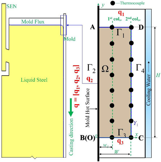
Figure 1.
Mold simulator apparatus and the locations of thermocouples inside the mold wall.
The mold heat transfer model is based on the following assumptions: (1) transverse heat flow perpendicular to the plane of interest is negligible [25], and (2) since the temperature of the mold wall ranges from 300 to 600 K [56], it is assumed that the material properties of the mold, such as heat capacity, density, and thermal conductivity, remain constant. Therefore, the heat transfer within the rectangular area ABCD of the mold, as shown in Figure 1, is considered to be two-dimensional. The problem of predicting the thermal field in a longitudinal section (ABCD) is referred to as the direct problem, and it is governed by the Fourier heat transfer partial differential equation with corresponding thermal boundary conditions.
It should be noted that the heat flux q* is unknown, leading to an underdetermined heat transfer problem that cannot be directly solved using Equations (1)–(4). In cases where the heat flux boundary conditions are not known but temperature measurements are available, an inverse heat-conduction problem should be formulated to address the underdetermined heat transfer issue.
2.2. Description of the Inverse Problem
In this study, the sequential regularization method (SRM) [57,58,59] is employed to solve the inverse heat-conduction problem for the determination of heat flux using the observed temperatures. The SRM approach involves two steps: (1) Temporarily assuming the heat fluxes are equal, qj = qj+1 = … = qj+r−1, for r future time steps from tj to tj+r−1; and (2) estimating qj for the time interval [tj, tj+r−1] by minimizing the square difference between the calculated temperatures T and the observed temperatures Y. Therefore, the inverse heat-conduction problem can be formulated as an optimization problem with PDE constraints [13]. That is,
All of the variables in the Equations (5)–(9) are dimensionless. The dimensionless quantities were defined as follows,
where r (≥1) is the number of future time steps. The Dirac delta function, δ(x), is defined such that it is equal to unity at x = 0 and is zero everywhere else. (xm, ym) represents the location of thermocouples. To solve the direct problem of the partial differential equation described by Equations (6)–(9), the finite difference method is used. This method involves discretizing the computational domain (Ω), represented by the rectangular area ABCD, into a grid of uniform size nx × ny. The boundaries Γ1, Γ2 and Γ3 are divided into n1 (=nx), n2 (=ny) and n3 (=nx) divisions, respectively. Then, the unknown heat flux qj (=[, , ]T) at time tj is a vector with N (= + + ) components. , , and are vectors of dimensions × 1, × 1 and × 1, corresponding to the heat fluxes on Γ1, Γ2, and Γ3, respectively. is the n-th component of heat flux qj at the time tj.
The right-hand side of Equation (5) contains a spatial regularization term, Rc(qj), which is used to reduce the spatial variation in the predicted heat flux [60]. There are three types of spatial regularizations: zeroth, first, and second order. Table 1 contains the standard forms of integration, Rc(qj), and their corresponding discrete form approximations, Rd(qj), for those three different orders of spatial regularization. The regularization parameter, denoted by α‘ (>0), is used to control the strength of regularization [38,39,40,41,42,43,44,45,46,47,48,49,57,59,61]. It should be noted that the heat flux, q, may be discontinuous at the intersection points of neighboring boundaries, such as points A and B in Figure 1. Therefore, the spatial regularizations for the heat flux of Γ1, Γ2, and Γ3 might be addressed separately.

Table 1.
Three different orders of spatial regularization methods.
2.3. Method of Solving the Inverse Problem
The discrete form analogous to the objective function Equation (5) could be rewritten as follows.
where both Yj and Tj are M × 1 temperature vectors at time tj, and M is the number of measurements. and are the measured and the calculated temperature at the position (xm, ym) of temperature measurement at time tj, respectively. ||·|| denotes the standard Euclidean norm. The parameter d represents the order of spatial regularization. hd is a dth-order derivative operator acting on the respective boundary heat flux (Table 1) [11,62,63]. α (>0) is the regularization parameter. There are various classical methods for selecting the regularization parameter, such as L-curve methods and Morozov’s discrepancy principle, which can be found in the literature [61,62,63,64,65]. However, the main focus of this study is to investigate the effects of the influences of a number of future time steps, regularization parameters, order of regularization, discrete grids, and time step size on the 2DIHCP accuracy. Therefore, the influence of the regularization parameter is determined through a trial-and-error approach in order to provide recommendations and guidance for selecting the appropriate α value.
In zeroth-order regularization (d = 0), hdqj indicates the magnitude of heat fluxes, and α||hdq||2 penalizes the amplitude of the heat flux. In first-order regularization (d = 1), hdqj can be interpreted as an approximation of the gradient of the heat flux. In second-order regularization (d = 2), hdqj can be interpreted as an approximation of the second derivative of the heat flux. Herein, the first-order regularization constrains solutions with large gradients, and the second-order regularization penalizes solutions that have considerable second derivatives. The performances of those three different regularization methods, along with the influence of the regularization parameter on the accuracy of the inverse problem calculation, will be discussed in further detail in Section 4.
Expanding the temperature field in a Taylor series about an assumed heat flux q*.
is the temperature calculated using the assumed heat flux q*. Usually, q* is an a priori estimate of qj. To our knowledge, q* can be set to zero if no a priori information about the heat flux is available, which will consequently reduce the computations required [11]. is called the M × N sensitivity coefficient matrix at time tj and is defined as follows.
To minimize the objective function given by Equation (11), it can be achieved by taking the partial derivative of Equation (11) with respect to the vector of qj, setting it to zero, and substituting from Equation (15). This yields an estimator for unknown heat flux qj.
2.3.1. Sensitivity Coefficient Matrix
The sensitivity coefficient represents the temperature rise at the sensor location (xm, ym) in response to a unit step change in the heat flux at point (xn, yn) on boundaries Γ1, Γ2, and Γ3, at time tj. According to the definition of sensitivity coefficient Equation (16), the sensitivity coefficient problem can be obtained by taking the partial derivative of Equations (6)–(9) with respect to a heat flux component , then yielding the governing sensitivity coefficient problem.
2.3.2. Stopping Criteria
If there is no measurement error in the temperature, the traditional stopping criteria for Equation (5) and/or Equation (11) are given by [64],
where and are user-prescribed tolerances.
2.3.3. Algorithm for Sequential Regularization Method
The algorithm of the sequential regularization method (SRM) solving the inverse problem is summarized in Table 2. The complete code base of this study is made available to the wider research community [66]. It is worth noting that the sensitivity coefficient matrix can be computed only once if Equations (18)–(21) are linear at step 5. Moreover, updating the heat flux qj using Equation (17) only once at step 8 might be sufficient in most cases to achieve accurate results.
Table 2.
Algorithm for solving 2DIHCP by sequential regularization method.
3. Model Verification
3.1. Validation for Solving Direct Problem and Sensitivity Coefficient Problem
In this study, the Crank–Nicolson (CN) semi-implicit scheme is employed to solve the partial differential equations of heat-conduction problem Equations (6)–(9) and the sensitivity coefficient problem given by Equations (18)–(21). This use of the CN semi-implicit difference scheme for solving heat-conduction problems has been well documented in the literature [67,68]. Prior to applying this method to inverse calculations, it is important to verify its accuracy in solving partial differential equations using the finite difference method (FDM). To do so, FDM numerical calculations for a two-dimensional heat transfer problem were compared with the analytical solution from a textbook [69]. The results of the FDM calculations were found to be in agreement with those of the analytical solution, indicating that FDM can accurately solve the partial differential equations related to heat conduction.
3.2. Validation for Inverse Problem
To ensure the reliability of the algorithm used for determining the boundary heat flux from temperature measurements, it is necessary to validate the process.
3.2.1. Methodology of Validation
The validation process involves the following steps: (1) Specify the analytic expression for a pre-set heat flux gexa(Γ2,t) on the boundary Γ2. (2) Specify the location of temperature sensors in the computation domain. As shown in Figure 1, The direct problem in this study involves the conduction of heat within a copper rectangular area labeled ABCD, with dimensions of 21 mm × 8 mm (height × width) and an initial temperature of 0 K. The boundaries Γ1, Γ3, and Γ4 are insulated. The domain Ω comprises two columns of 2 × 8 thermocouples. The first column consists of eight thermocouples spaced 3 mm apart in the vertical direction and located 3 mm away from AB. The second column comprises eight thermocouples spaced 3 mm apart in the vertical direction and situated on the boundary on the boundary Γ4 (CD). (3) Generate the simulated measured temperature data. The pre-set heat flux gexa(Γ2,t) is applied on the boundary Γ2. Then, the direct problem given by Equations (6)–(9) is solved to compute the temperature. The temperatures of the thermocouples are measured at intervals of 0.1 s, where the sampling frequency of temperature fs is 10 Hz. (4) The reconstruction of heat flux. Substitute the measured temperatures into the above inverse problem algorithm (Table 2) to estimate the heat flux (gpred), and (5) evaluate the accuracy of the inverse analysis. The following relative error between the exact and the reconstructed result is employed to evaluate the accuracy of heat flux estimations [69],
where gexa and gpred are the exact and the predicted heat fluxes, respectively. A high value of the relative error, epred, indicates that the reconstructed heat flux is of lower accuracy. It is important to note that having a temperature residual (||Y−T||) equal to zero does not guarantee that the relative error between the reconstructed and exact heat flux is also zero. In other words, even if the calculated temperatures closely match the measured ones, the reconstructed heat flux may not necessarily match the exact heat flux due to the inherent instability, non-uniqueness, or non-existence of inverse problem solutions.
3.2.2. Validation
To validate the accuracy of the SRM-based inverse problem, three different cases of heat fluxes were considered. In Case 1, a time-spatial periodically varying heat flux was used to assess the accuracy of the inverse problem. The time-spatial periodically varying heat flux on the boundary Γ2 is,
where A0 is 1 × 10⁶ W·m−2, H is 0.021 m, and is 20 s.
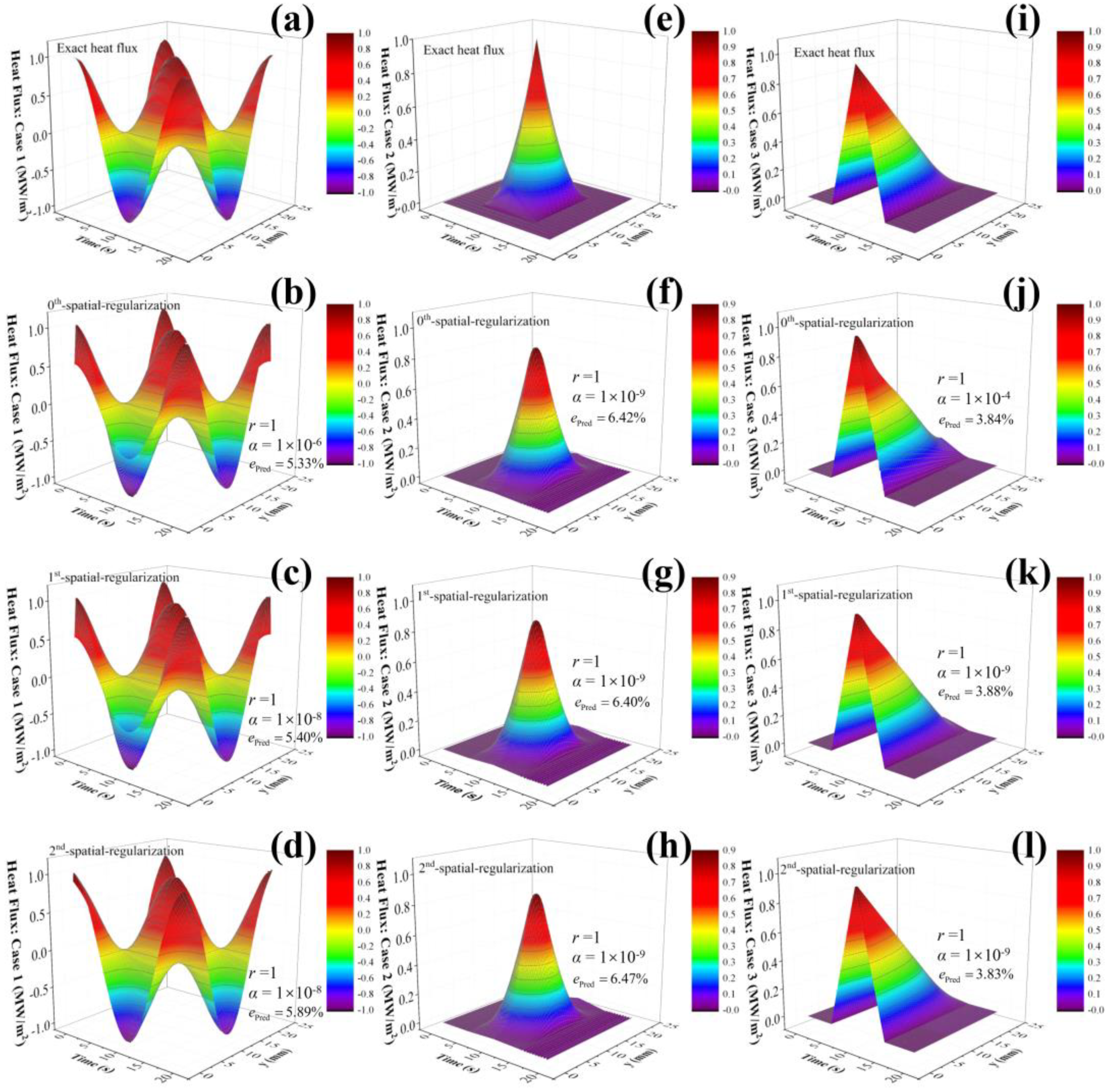
Figure 2a–d show the exact Case 1 value and the predicted value obtained with the SRM-based inverse problem with zeroth-, first-, and second-order spatial regularization. The tolerances of , and are 10−3 and 10−6 for the 2DIHCP calculation. The relative error (epred) was found to be 5.33% (Figure 2b), 5.40% (Figure 2c), and 5.89% (Figure 2d) for zeroth-, first-, and second-order spatial regularization, respectively, when compared to the exact Case 1 value. It suggests the proposed SRM-based inverse problem is capable of reconstructing the time-spatial periodically varying heat flux from the observed temperatures of a mold.

Figure 2.
Case 1: (a) the exact heat flux; the predicted by inverse problem with (b) zeroth-, (c) first-, and (d) second-order spatial regularization; Case 2: (e) the exact heat flux; the predicted by inverse problem with (f) zeroth-, (g) first-, and (h) second- order spatial regularization; Case 3: (i) the exact heat flux; the predicted by inverse problem with (j) zeroth-, (k) first-, and (l) second-order spatial regularization.
Case 2: a heat flux function with a step change or a sharp corner was considered, which is generally difficult to recover through inverse analysis. To assess the most stringent test conditions, we considered the heat flux involving a triangular variation in both time and space. That is,
With , and . Where A0 is 1 × 10⁶ W·m−2, l0, l1, l2, and l3 is 0.007, 0.003, 0.010, and 0.017 m, , , and is 5, 10, and 15 s, respectively.
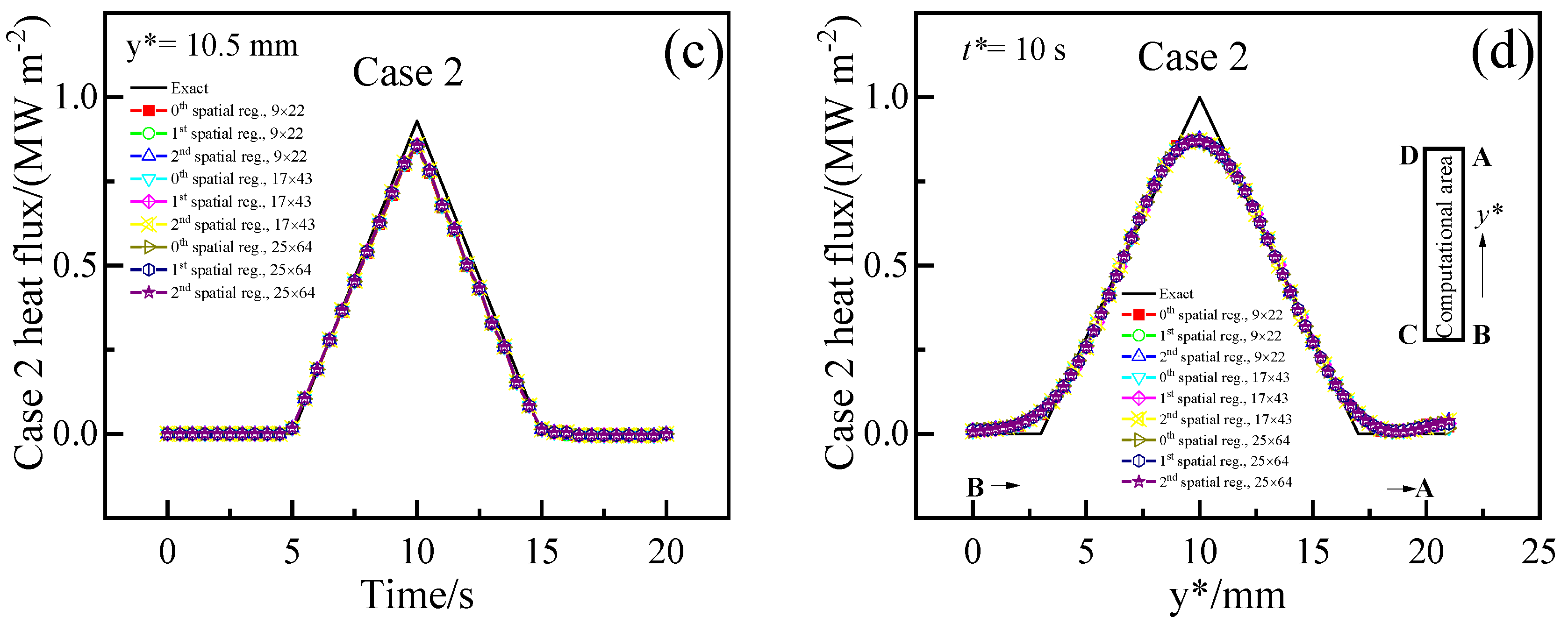
Figure 2e–h show the exact Case 2 value and the predicted values obtained with the SRM-based inverse problem with zeroth-, first-, and second-order spatial regularization, respectively. Compared with the Case 2 exact value (Figure 2e), the relative error (epred) was found to be 6.42% (Figure 2f), 6.40% (Figure 2g), and 6.47% (Figure 2h) or zeroth-, first-, and second-order spatial regularization, respectively. It is implied that the present SRM-based inverse problem can reconstruct the boundary heat flux involved in a triangular variation in both time and space.
Case 3: a heat flux featuring only a triangular variation in time was considered.
where A0 is 1 × 10⁶ W·m−2, H is 0.021 m, , , , and is 5, 10, 15, and 20 s, respectively.
Figure 2i–l show the exact Case 3 value and the predicted values obtained with the SRM-based inverse problem with zeroth-, first-, and second-order spatial regularization, respectively. Compared with the Case 3 exact value (Figure 2i), the relative error (epred) was found to be 3.84% (Figure 2j), 3.88% (Figure 2k), and 3.83% (Figure 2l) for zeroth-, first-, and second-order spatial regularization, respectively. It is demonstrated that the SRM-based inverse problem can accurately reconstruct the boundary heat flux featuring only a triangular variation in time.
Overall, the results demonstrate that the proposed SRM-based inverse problem is capable of accurately reconstructing time-spatial periodically varying heat fluxes, heat fluxes with a triangulation variation in both temporal and spatial domains, and heat fluxes with only a triangular variation in time from the measured temperatures.
4. Results and Discussion
The SRM-based inverse problem involves the choice of many parameters, i.e., the number of future time steps (r), the regularization parameter (α), the order of spatial regularization (d), the number of discrete grids, and time step size. The performances of those SRM parameters are investigated in this section in order to provide recommendations and guidance for the selection of those parameters. For this purpose, 2376 different tests were carried out using a trial-and-error approach in which each parameter was varied as listed in Table 3, while the other parameters were held constant. All the computations are carried out by a computer with an Intel(R) Core (TM) i7-9700K CPU @ 3.60 GHz and 32 GB RAM memory. Subsequently, the influence of these SRM parameters on the accuracy of the inverse problem was analyzed.
Table 3.
Parameters variation in the inverse problem for the test case.
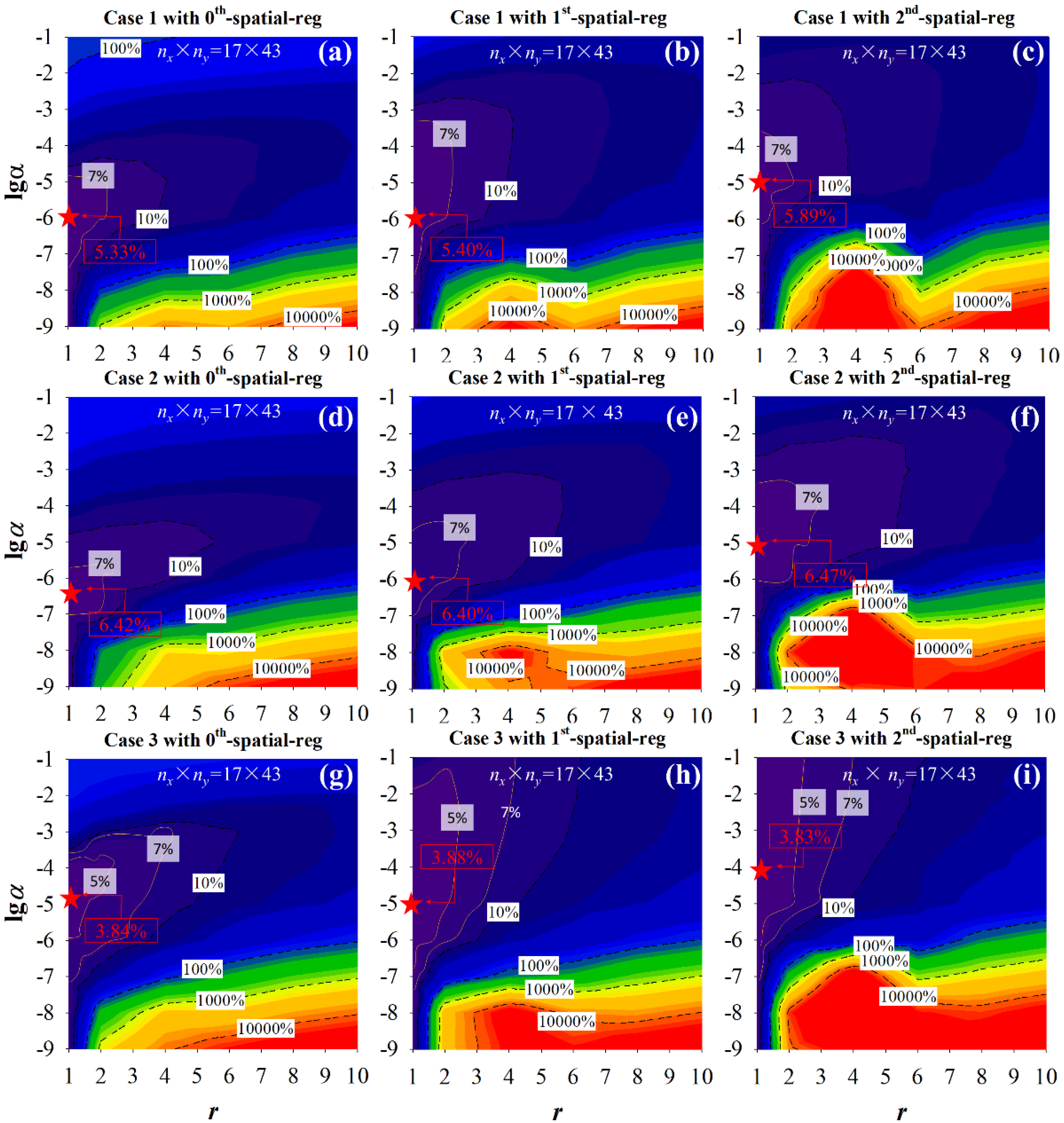
Figure 3 shows the accuracy of the inverse problem, as characterized by the relative error (epred), for the estimation of Cases 1, 2, and 3 heat flux. The time step was 0.05 (1/2fs) seconds, and the discrete grids were 17 × 43 for the calculations. The results indicate that the number of future time steps (r), the regularization parameter (α), and the order of spatial regularization (d) all influence epred. Generally, any values of r and α that produce a relative error of less than 10.0% could be demonstrated as a feasible solution for selecting r and α [57]. The absence of spatial regularization (α is 0) leads to epred above 10.0%. The optimal range for r is 1 to 4, while the optimal range for α is 10−7 to 10−4, which is consistent with previous studies [11,38].

Figure 3.
Effects of the number of future time steps (r) and the regularization parameter (α) on the relative error (epred) of the reconstructed heat fluxes. (a–c) are the relative errors for Case 1 heat flux; (d–f) are that for Case 2 heat flux; (g–i) are that for Case 3 heat flux. ★ denotes the location of minimum epred.
4.1. Effect of Number of Future Time Steps
We illustrated two strict test conditions, Case 1 and Case 2, to evaluate the impacts of the number of future time steps on the accuracy of inverse analysis. Case 1 involved a heat flux with a periodic variation in time-spatial (Equation (25)), while Case 2 had a heat flux with a triangular variation in time-spatial (Equation (26)).
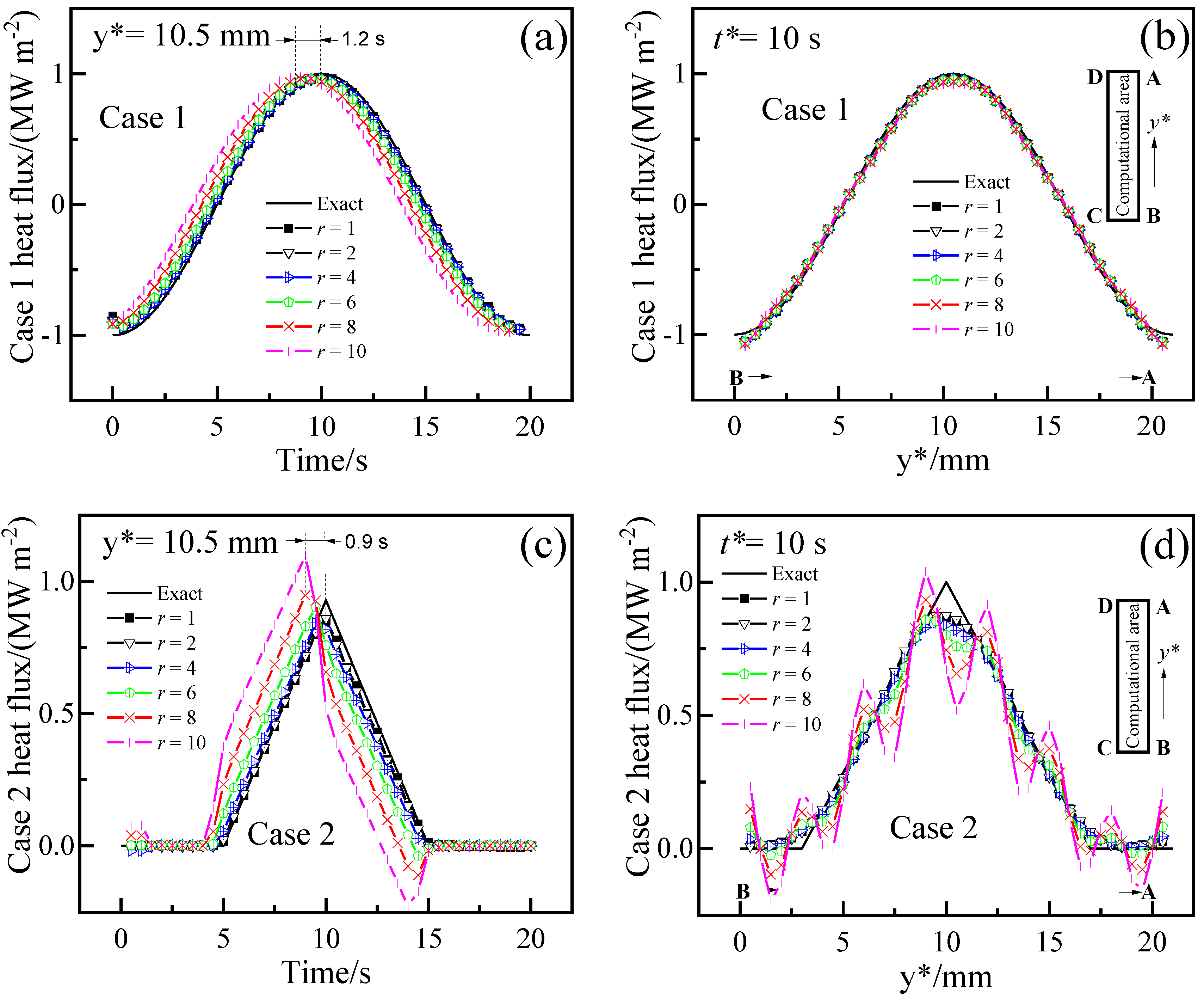
Figure 4 shows the changes in reconstructed heat fluxes at a specific location (y is 10.5 mm) and time (10 s) via 2DIHCP calculations with varying numbers of future time steps (r). The 2DIHCP calculations used zeroth-order spatial regularization (α is 1 × 10⁻⁶), a time step of 0.05 (1/2fs) seconds, and 17 × 43 discrete grids. For Case 1, the predicted heat fluxes were in agreement with the exact one. However, a phase shift phenomenon is observed where the peak of predicted heat flux rose earlier than that of the exact one and then decreased before it. This phenomenon is attributed to the sequential regularization method, which utilizes future time data to stabilize the solution [11]. The phase difference between the reconstructed results and the exact is 0.2, 0.2, 0.2, 0.4, 0.7, and 1.2 s, which corresponds to the heat flux predicted by inverse analysis with the number of future time steps (r) is 1, 2, 4, 6, 8, and 10, respectively. The phase difference between the reconstructed results and the exact one increases with the number of future time steps (r).

Figure 4.
Comparison of the heat fluxes reconstructed using different numbers of future time steps (r). (a) Case 1 heat flux at y = 10.5 mm; (b) Case 1 heat flux when time is 10 s; (c) Case 2 heat flux at y = 10.5 mm; (d) Case 2 heat flux when time is 10 s.
The deviation between the reconstructed heat fluxes and the exact value at the beginning of time can be attributed to the inaccuracy of the initial guess of heat flux (q* is 0) at time 0 [11]. At the end of time, the deviation between the reconstructed results and the exact one was due to the use of the sequential regularization method, which uses the measured temperature of future time steps to improve the stability of the solution, resulting in the heat flux at the end of time not being updated. Additionally, as demonstrated in Figure 4b, the reconstructed heat fluxes may deviate from the exact value at the locations of B (y* is 0) and A (y* is 21 mm). This discrepancy could be explained by the fact that the discontinuity and non-differentiability of the heat flux at points B and A make the inverse calculation of the sequential regularization method difficult. However, this potential shortcoming can be circumvented by utilizing an earlier initial time and a larger computational domain than that originally required [27,53,62].
For Case 2, as demonstrated in Figure 4c,d, the reconstructed heat fluxes match the exact one for r is 1, 2, and 4 but exhibit significant deviation for r is 6, 8, and 10. The deviation between the reconstructed results and the exact one increases with increasing r. The phase difference between the calculated Case 2 heat flux and the exact is also observed. The phase difference is 0.2, 0.2, 0.3, 0.5, 0.7, and 0.9 s that is corresponding to r is 1, 2, 4, 6, 8, and 10, respectively. Additionally, the reconstructed heat fluxes may also be inaccurate at the beginning and end of time. In addition, there is a lack of agreement between the exact heat flux and the recovered one at the locations of y* is 3, 10, and 17 mm, where the exact heat flux has sharp spatial changes (Figure 4d). This could be attributed to the fact that a sharply changing heat flux is not differentiable, and the spatial regularization term in the inverse problem (Equation (5)) penalizes sharp changes in the reconstructed heat flux in space.
In summary, the phase shift phenomenon is observed, where the predicted peak of heat flux rises earlier than the exact one and then decreases before it. The phase difference increases with the number of future time steps. The reconstructed heat fluxes can deviate from the exact value at the beginning and the end of the time. Additionally, the reconstructed heat flux may not be in suitable agreement with the exact one when the exact heat flux has sharp spatial changes.
4.2. Effect of Regularization Parameter
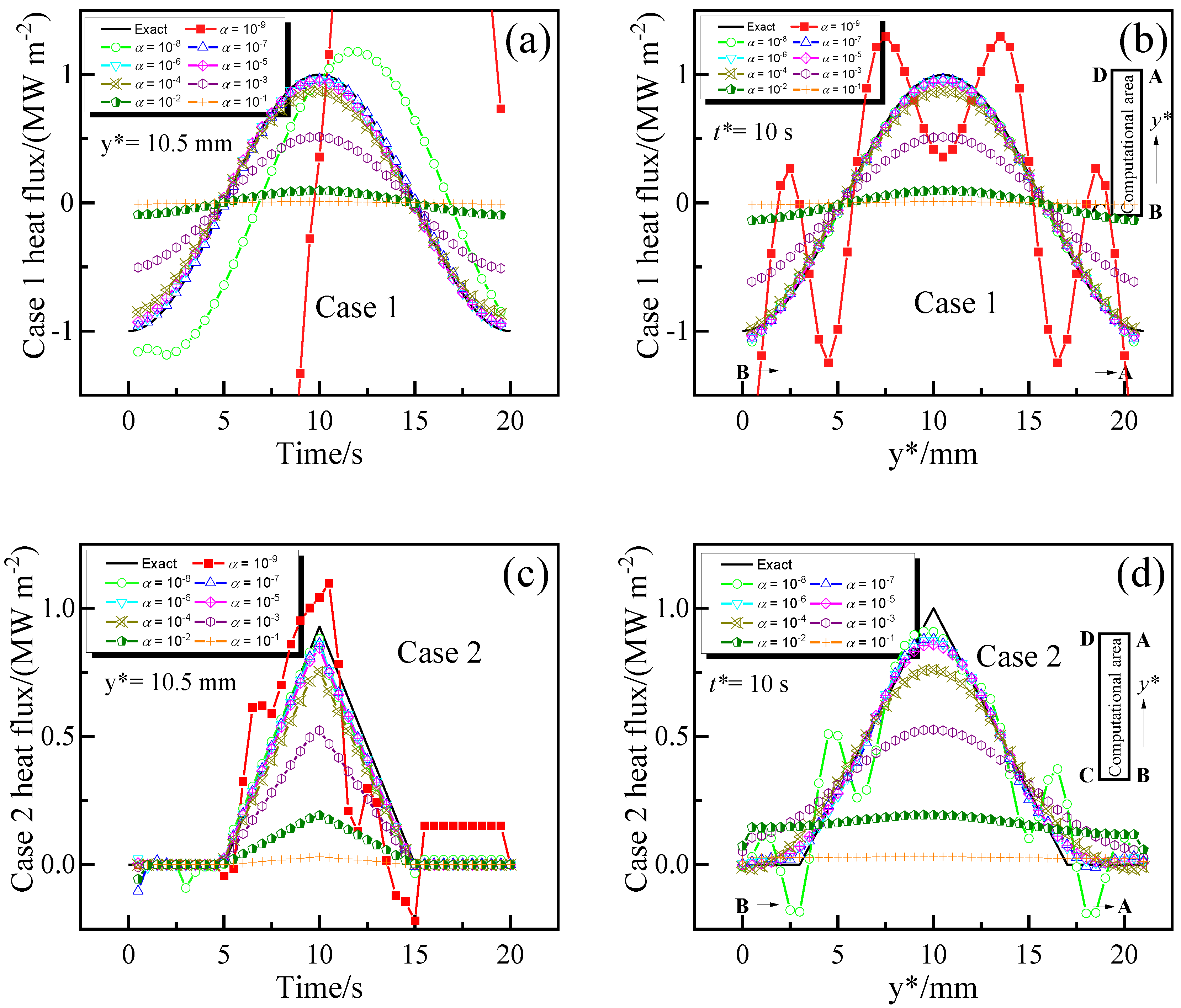
We illustrated two strict test conditions, Case 1 and Case 2, to evaluate the effect of the regularization parameter (α) on the accuracy of inverse analysis. Figure 5 shows the changes of heat fluxes at the location with y is 10.5 mm and at the time of 10 s reconstructed via 2DIHCP calculations with varying the regularization parameter. The 2DIHCP calculations utilized a single future time step, zeroth-order spatial regularization, a time step of 0.05 (1/2fs) seconds, and 17 × 43 discrete grids.

Figure 5.
Comparison of the heat fluxes reconstructed using different regularization parameters (α). (a) Case 1 heat flux at y = 10.5 mm; (b) Case 1 heat flux when time is 10 s; (c) Case 2 heat flux at y = 10.5 mm; (d) Case 2 heat flux when time is 10 s.
The predicted Case 1 heat fluxes match the exact one for α values ranging from 10−7 to 10−4 (Figure 5a,b). For α values less than 10−7, the heat flux behavior becomes unstable and oscillatory. Conversely, for larger values of α (>10−4), the heat flux remains smooth with only slight changes and is thus fixed to the initial guess values (q* is 0). This result is consistent with previous research by Vogel [64] and Hansen [65]. Similarly, Figure 5c,d demonstrate that the predicted Case 2 heat fluxes are generally consistent with the exact one when α is in the range of 10−7 to 10−4. However, the predicted heat fluxes may differ from the exact value when the exact heat flux presents sudden spatial changes at the locations of y* is 3, 10, and 17 mm (Figure 5d). This discrepancy may also be attributed to the fact that heat flux containing sharp variations is not differentiable, and the spatial regularization limits the sharp changes of the reconstructed heat flux. In summary, a small value of the regularization parameter (α) leads to oscillatory behavior and instability of the heat flux. On the other hand, a large value of α results in the heat flux remaining very smooth and only changes a little and thus will be fixed to the initial guess values.
4.3. Effect of Spatial Regularization Method (d) and Discrete Grids (nx × ny)
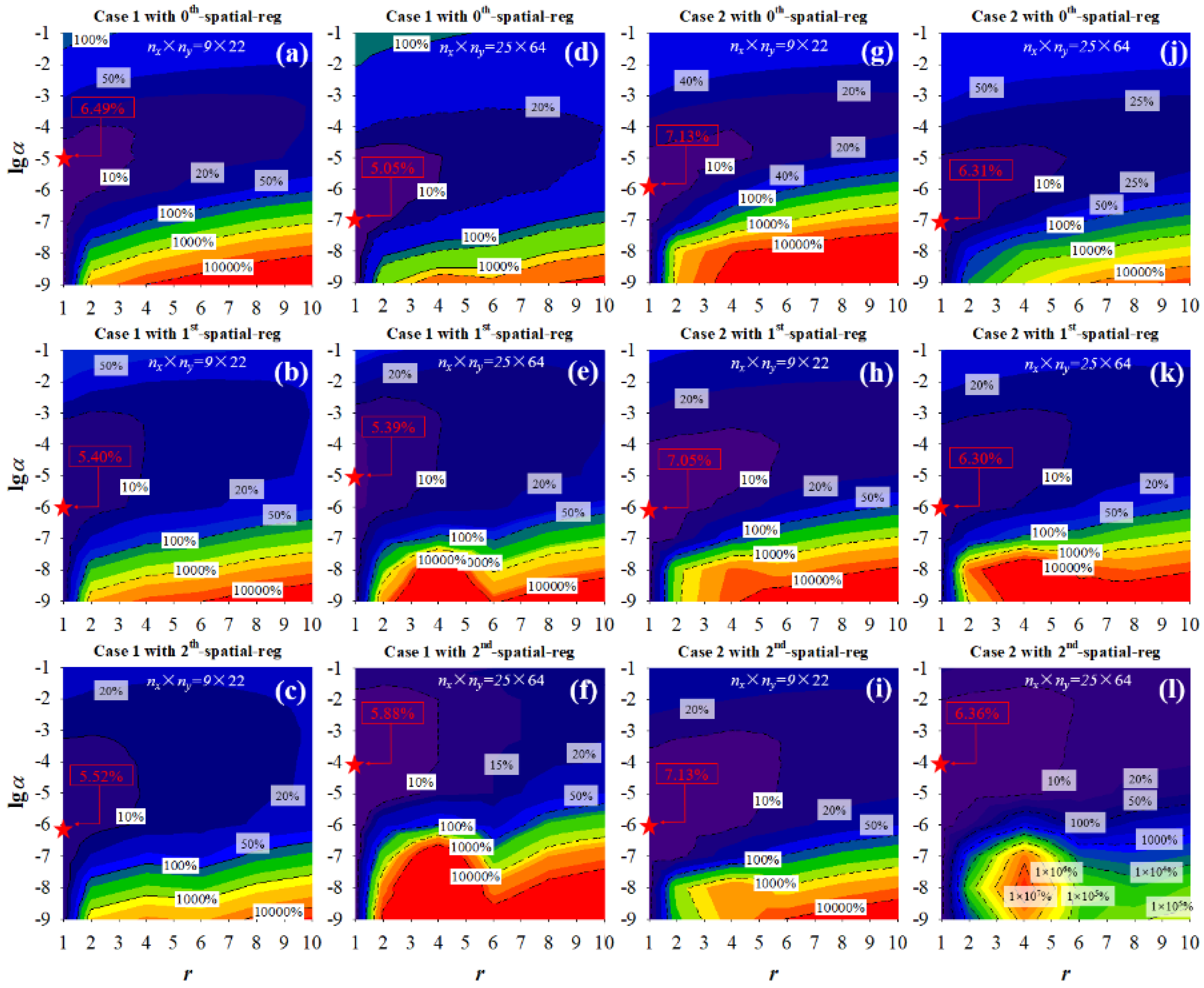
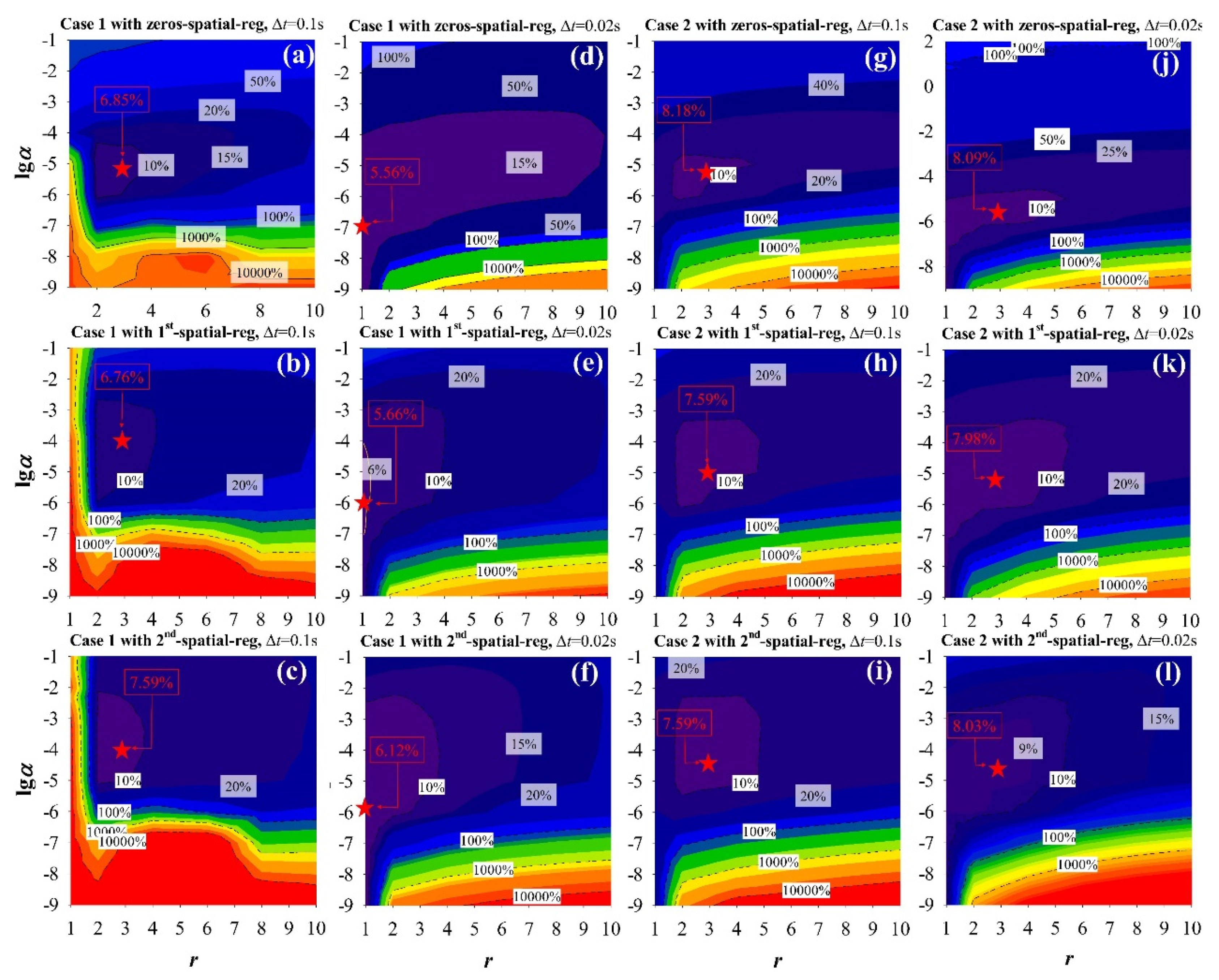
The effects of the spatial regularization method (d) and discrete grids (nx × ny) on the accuracy of inverse analysis are also investigated by the discussion of Case 1 and Case 2. Figure 6 shows the relative error (epred) of the estimated heat fluxes in Case 1 and Case 2 using 2DIHCP with different order of spatial regularization (d) and the number of discrete grids, while the time step is 0.05 (1/2fs) seconds. It is general that any values of r and α in the region yielding epred less than 10.0% can be considered a feasible solution for selecting r and α [56]. The optimal number of future time steps (r) is found to be between 1 and 4, and the optimal range of α is 10−7 to 10−4, which is consistent with the findings in Figure 3.

Figure 6.
Effects of the number of future time steps (r) and the regularization parameter (α) on the relative error (epred). (a–c) Case 1 reconstructed using 9 × 22 discrete grids, (d–f) Case 1 reconstructed using 25 × 64 discrete grids, (g–i) Case 2 reconstructed using 9 × 22 discrete grids, and (j–l) Case 2 reconstructed using 25 × 64 discrete grids. ★ denotes the location of minimum epred.
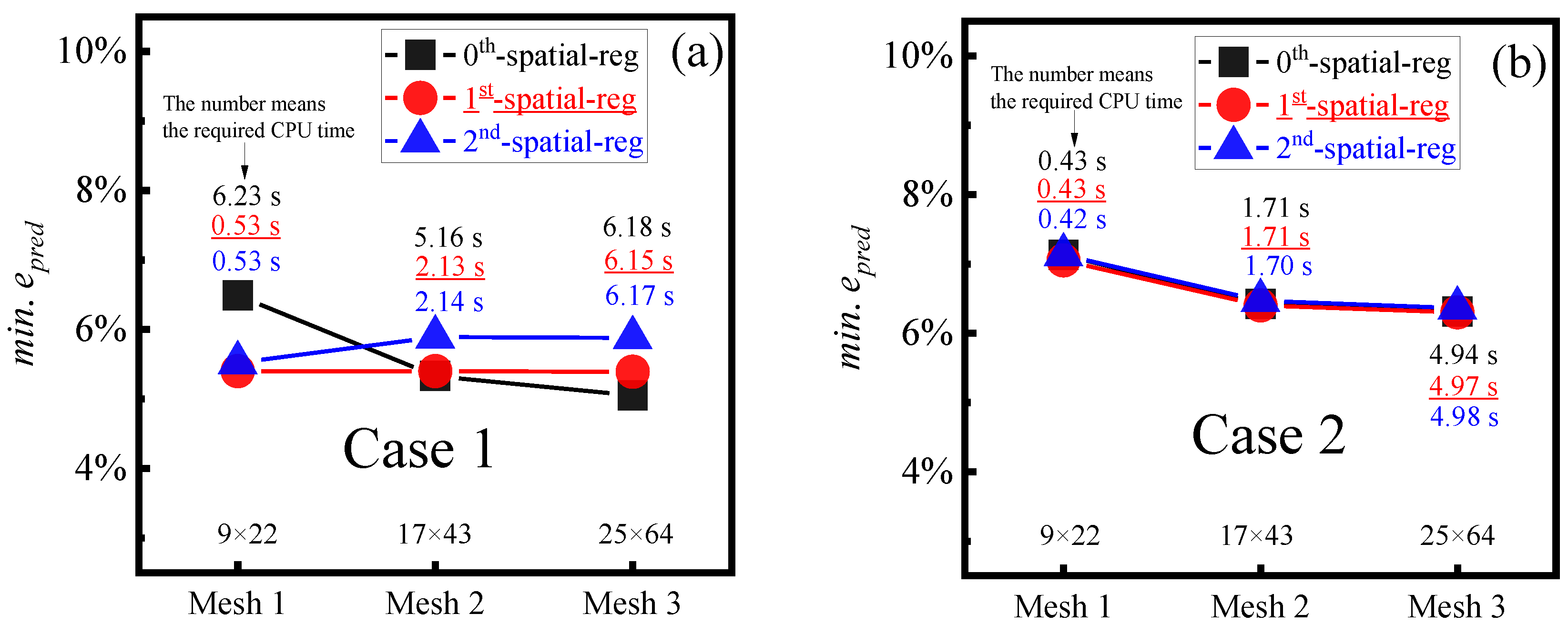
Figure 7 shows the minimum epred and the required computing time (CPU time) of heat fluxes reconstructed by the inverse analysis with different SRM parameters. At the same time, the optimal r and α of those heat flux estimations corresponded to the location of minimum epred (marked with a star ★) in Figure 6. When a 9 × 22 discrete grid is used, the minimum epred of the predicted Case 1 heat flux is 6.49%, 5.40%, and 5.52% for zeroth-, first-, and second-order order spatial regularization, respectively. The corresponding values for the predicted Case 2 heat flux are 7.13%, 7.05%, and 7.13%. By using a finer mesh grid of 25 × 64 discrete grids, the minimum epred of the predicted Case 1 heat flux is 5.05%, 5.39%, and 5.88% for zeroth-, first-, and second-order spatial regularization, respectively. The corresponding values for the predicted Case 2 heat flux are 6.31%, 6.30%, and 6.36%. It is noteworthy that zeroth- and first-order spatial regularizations provide more accurate results than second-order spatial regularization, and the accuracy of zeroth-order regularization is comparable to that of first-order regularization.

Figure 7.
Effect of the grid points (nx × ny) on the minimum epred and CPU time. (a) Case 1; (b) Case 2.
Reconstructing heat flux with sharp changes is more challenging than that with smooth changes due to the lack of differentiability, as demonstrated in Case 2. As shown in Figure 7, using 9 × 22 discrete grids, the minimum epred of the predicted Case 2 heat flux is 7.13%, 7.05%, and 7.13% for zeroth-, first-, and second-order spatial regularization, respectively. The corresponding values for a finer grid of 25 × 64 are 6.31%, 6.30%, and 6.36%. It is demonstrated that first-order spatial regularization yields a higher accuracy for the reconstruction of the heat flux containing sharp spatial variations when compared to both zeroth- and second-order spatial regularizations.
Using a finer grid generally leads to more accurate results, except for Case 1 with second-order spatial regularization. For example, with first-order spatial regularization, the minimum epred of the predicted Case 2 heat flux is 7.05%, 6.40%, and 6.30% for the discrete grids of 9 × 22, 17 × 43, and 25 × 64, respectively. However, a finer grid can bring about two contradictory outcomes: for one thing, it can minimize the truncation errors of FDM solving PDE, thereby enhancing the accuracy of the inverse problem; for another thing, it can lead to the accumulation of FDM truncation errors and rounding errors as well as an increase in the freedom degree of the objective function, thus reducing the accuracy of the inverse problem [11,35]. In this study, the former effect of increasing accuracy might be more pronounced than that of the latter effect, thus leading to an improvement in accuracy as the grid was refined for the majority of tests.
Using a coarser grid reduces the CPU time required for inverse analysis. For example, with first-order spatial regularization, the CPU time of the predicted Case 2 heat flux is 0.43, 1.71, and 4.97 s for the discrete grids of 9 × 22, 17 × 43, and 25 × 64, respectively. The effect of the order of spatial regularization on CPU time is not significant. For example, with 17 × 43 discrete grids, the CPU time of the predicted Case 2 heat flux is 1.71, 1.71, and 1.70 s for zeroth-, first-, and second-order spatial regularization, respectively. Similarly, for predicted Case 1 heat flux with 25 × 64 discrete grids, the CPU time is 6.18, 6.15, and 6.17 s for zeroth-, first-, and second-order spatial regularization, respectively.
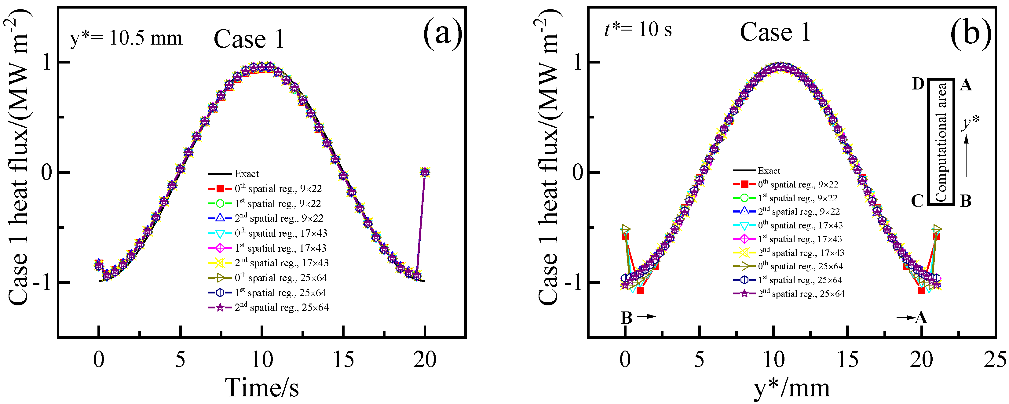
Figure 8 shows the changes of heat fluxes at the location with y is 10.5 mm and at the time of 10 s reconstructed via 2DIHCP calculations using different orders of spatial regularization (d) and discrete grids. The time step for the calculations was 0.05 (1/2fs) seconds, and the optimal r and α of those heat flux estimations corresponded to the location of minimum epred (★) in Figure 6.

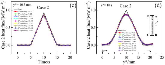
Figure 8.
Comparison of the heat fluxes reconstructed with different order of spatial regularization (d) and the grid pints (nx × ny). (a) Case 1 heat flux at y = 10.5 mm; (b) Case 1 heat flux when time is 10 s; (c) Case 2 heat flux at y = 10.5 mm; (d) Case 2 heat flux when time is 10 s.
For Case 1, the results in Figure 8a indicate that if the initial guess heat flux is far from the correct value, the reconstructed heat flux can deviate from the exact value at the beginning and end of the time, which the findings are similar to the results from Figure 4. Figure 8b shows that the reconstructed Case 1 heat fluxes can deviate from the exact value at locations of B (y* = 0) and A (y* = 21 mm). This might be attributed to the discontinuity of the heat flux at the C-B-A-D boundary and the lack of differentiability of the heat flux at B and A, which makes the inverse analysis difficult. For Case 2, Figure 8c shows the predicted heat fluxes roughly match the exact one, except at the time of 10.5 s when the exact heat flux exhibits a sharp spatial change. This suggests that the temporal accuracy of the reconstructed heat fluxes is satisfactory. On the other hand, the reconstructed heat fluxes can deviate from the exact value when the exact heat flux exhibits a sharp spatial change at locations of y* are 3, 10, and 17 mm in Figure 8d. This indicates that the spatial accuracy of the inversion results is inadequate due to the non-differentiability of the sharply changing heat flux, which limits the sharp spatial change in the reconstructed heat flux.
In summary, zeroth- and first-order spatial regularizations have higher accuracy than second-order spatial regularization, and the accuracy of zeroth order is comparable to that of first-order. Reconstructing sharply changing heat flux is more challenging than smoothly changing heat flux, and first-order spatial regularization yields higher accuracy for heat fluxes with sharp spatial variations. Using a coarser grid reduces the CPU time for inverse analysis compared to using a finer grid. The effect of the order of spatial regularization on CPU time is not significant.
4.4. Effect of Time Step Size (dt)
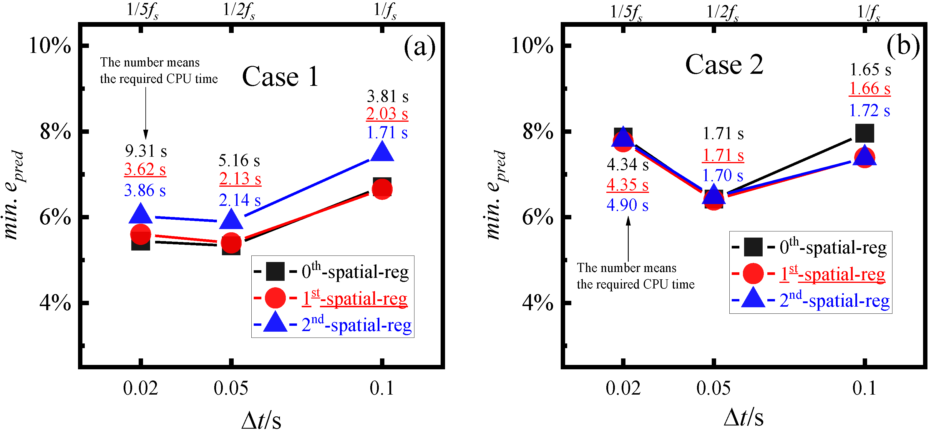
The effect of the time step size (dt) was also investigated by the discussion of two strict test conditions, Case 1 and Case 2. Figure 9 illustrates the accuracy of the inverse problem, as characterized by the relative error (epred), for the estimation of heat fluxes using 2DIHCP with 17 × 43 discrete grids and different the time step size (0.1 (1/fs), 0.05 (1/2fs) and 0.02 (1/5fs) seconds). The minimum epred and the CPU time of heat fluxes reconstructed are listed in Figure 10.

Figure 9.
Effects of time steps on the relative error (epred) of the predicted heat fluxes. (a–c) Case 1 heat flux reconstructed with time steps 0.1 s (1/fs); (d–f) Case 1 heat flux reconstructed with time steps 0.02 s (1/5fs); (g–i) Case 2 heat flux reconstructed with time steps 0.1 s (1/fs); (j–l) Case 2 heat flux reconstructed with time steps 0.02 s (1/5fs). ★ denotes the location of minimum epred.

Figure 10.
Effect of the time step on the minimum epred and CPU time. (a) Case 1; (b) Case 2.
The minimum epred initially decreases and then increases as the time step size decreases. For example, the minimum epred of Case 2 heat flux with zeroth-order spatial regularization is 7.96%, 6.42% 7.87% for time step sizes of 1/fs, 1/2fs, and 1/5fs, respectively. The utilization of small-time step size (dt) can bring about two contradictory outcomes: on the one hand, it can minimize the truncation errors of FDM solving PDEs, thereby enhancing the accuracy of the inverse problem; on the other hand, it can lead to the accumulation of FDM rounding errors and truncation errors, thus reducing the accuracy of the inverse problem. As a consequence, those two combined effects make the time step size of 1/2fs provide more accurate results than those calculations with the time step sizes of 1/fs and 1/5fs.
The CPU time required for inverse analysis increases with the decrease in time step size (dt). Using a smaller time step size also means that more temperature data points are collected, which can increase the computational cost and processing time. For example, with 17 × 43 discrete grids and first-order spatial regularization, the CPU time of the predicted Case 2 heat flux is 1.66, 1.71, and 4.35 s for the time step size of 1/fs, 1/2fs, and 1/5fs, respectively; the corresponding values for the predicted Case 1 heat flux with first-order spatial regularization are 2.03, 2.13, and 3.62 s.
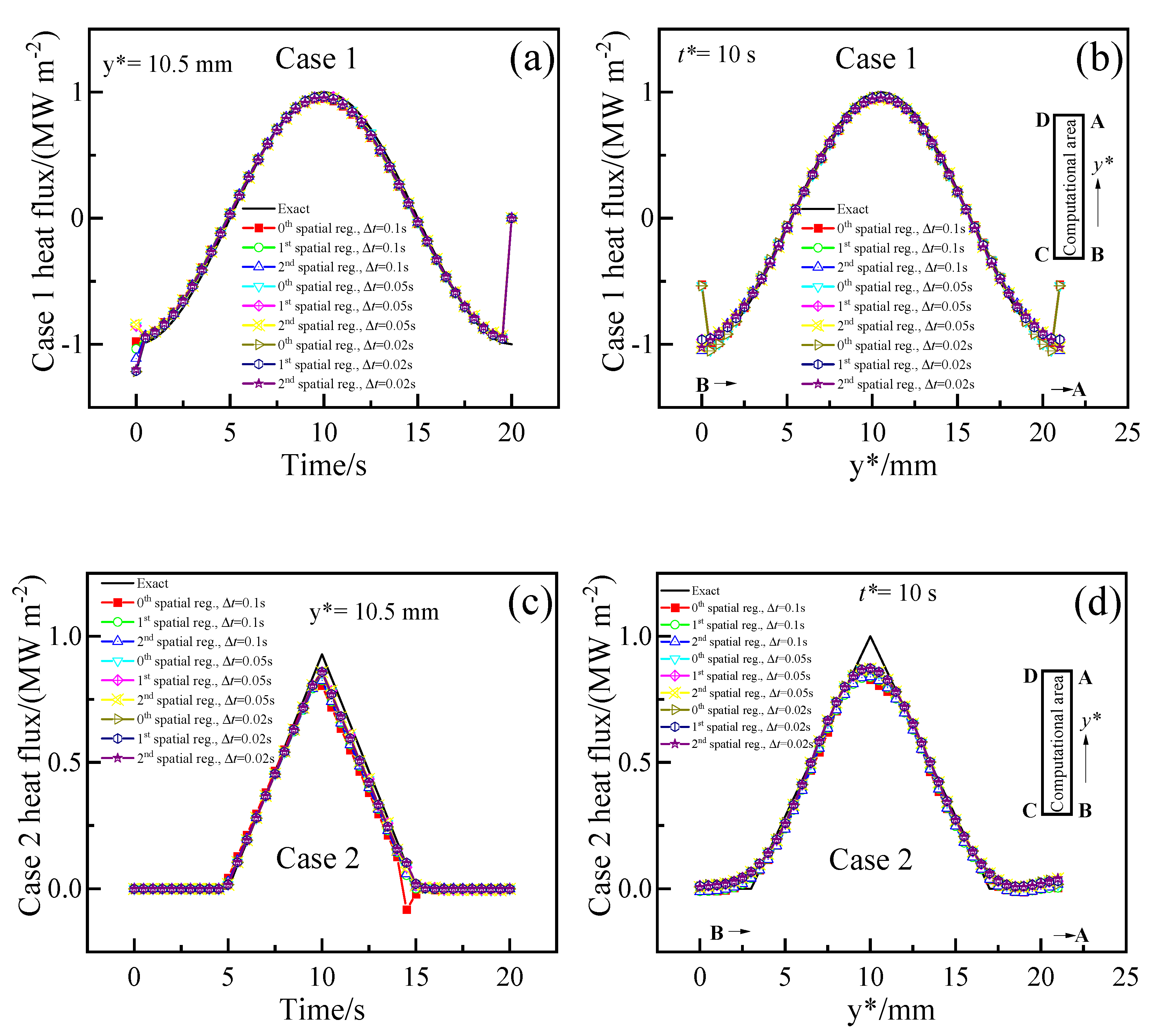
Figure 11 shows the changes of heat fluxes at the location with y is 10.5 mm and at the time of 10 s reconstructed by inverse analysis using varied time step sizes. In contrast, the optimal r and α of those heat flux estimations corresponded to the location of minimum epred (★) in Figure 9. For Case 1, as shown in Figure 11a, the reconstructed heat fluxes can deviate from the exact at the beginning and the end of the time. Figure 11b shows the reconstructed heat fluxes can deviate from the exact at the locations of B (y* is 0) and A (y* is 21 mm). For Case 2 (Figure 11c,d), the recovered heat fluxes can deviate from the exact when the exact heat flux exhibited a sharp spatial change at a time of 10.5 s, and the locations of y* are 3, 10, and 17 mm. This could also be attributed to the fact that the heat flux containing sharp variation is not differentiable, and the spatial regularization limits the sharp change in reconstructed heat flux. These findings are consistent with the results presented in Figure 4, Figure 5, and Figure 8.
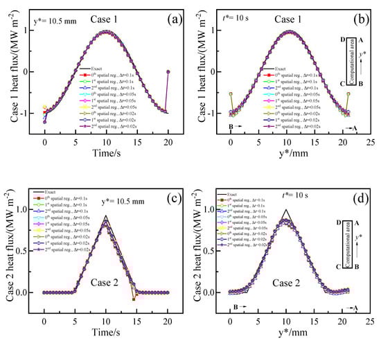
Figure 11.
Comparison of the heat fluxes reconstructed with different time steps (0.1 (1/fs), 0.05 (1/2fs) and 0.02 (1/5fs) seconds). (a) Case 1 heat flux at y = 10.5 mm; (b) Case 1 heat flux when time is 10 s; (c) Case 2 heat flux at y = 10.5 mm; (d) Case 2 heat flux when time is 10 s.
In brief, the accuracy of the inverse analysis first improves and then worsens as the time step size decreases. The time step size of 1/2fs provided a more accurate result than those of time step sizes of 1/fs and 1/5fs. However, decreasing the time step size increased the CPU time required for the inverse analysis. The proposed SRM-based IHCP offers several advantages: (1) high time resolution (due to the introduction of Beck’s future time step, as illustrated in Figure 7); (2) high spatial resolution and could deal with the discontinuity function form of the unknown heat flux, which is achieved through the incorporation of the spatial regularization term (observed in Figure 4, Figure 5, Figure 8, and Figure 11); and (3) fast due the nature of the sequential method: updating the heat flux using Equation (17) only once might be sufficient in most cases to achieve accurate results. Nevertheless, a significant limitation emerges in the form of a small-time step utilization. When employing a small-time step in the analysis (as depicted in Figure 10), the sensitivity coefficient J diminishes, resulting in an ill-posed scenario with Equation (17).
5. Conclusions
The study is to reconstruct the profile of an unknown continuous casting mold heat flux using measured temperature data. To address this problem, the study formulated a two-dimensional transient inverse heat-conduction problem (2DIHCP). Then, the study employed the sequential regularization method (SRM) with zeroth-, first-, and second-order spatial regularization to solve the 2DIHCP. The accuracy of the 2DIHCP was investigated under two strict test conditions, including Case 1, with time-spatially periodic heat flux, and Case 2, featuring a sharply changing heat flux. The effects of the number of future time steps, regularization parameters, order of regularization, discrete grids, and time step size on the accuracy of the 2DIHCP were analyzed. The following conclusions can be drawn:
- Increasing the number of future time steps results in a more pronounced phase shift between the peak of the predicted heat flux and the exact heat flux, where the predicted peak of heat flux rises earlier than the exact one and then decreases before it;
- Zeroth- and first-order spatial regularization provides higher accuracy than second-order spatial regularization, and zeroth-order regularization has comparable accuracy to first-order regularization;
- Reconstructing a sharply changing heat flux is more challenging than reconstructing a smoothly changing heat flux. First-order spatial regularization provides better accuracy for reconstructing heat flux with sharp spatial variations than both zeroth- and second-order spatial regularization;
- Using a coarser grid reduces the CPU time required for inverse analysis. The impact of the order of spatial regularization on CPU time is not significant;
- Decreasing the time step size initially increases the accuracy of inverse analysis, but after a certain point, the accuracy starts decreasing, and the CPU time required increases. The time step size of 1/2fs is recommended, where fs is the sampling rate of temperature.
Author Contributions
Conceptualization, H.Z. and P.X.; methodology, P.X.; software, H.Z.; validation, J.Z. and P.X.; formal analysis, J.Z.; investigation, H.Z.; resources, P.X.; data curation, P.X.; writing—original draft preparation, H.Z.; writing—review and editing, P.X.; visualization, P.X.; supervision, H.Z.; project administration, H.Z.; funding acquisition, H.Z. All authors have read and agreed to the published version of the manuscript.
Funding
This work was supported by NSFC (no. 52074135), the Jiangxi Provincial Natural Science Foundation (no. 20224ACB214011), and the Youth Jinggang Scholars Program in Jiangxi Province (QNJG2020049).
Data Availability Statement
The data presented in this study are available within the article.
Acknowledgments
The authors are grateful to Senlin Xie, Longyun Xu and Chao Fan for providing essential technical requirements and information for the practical of slab continuous casting.
Conflicts of Interest
The authors declare no conflict of interest.
Nomenclature
| c | heat capacity (J/kg·K) |
| d | order of spatial regularization, i.e., zeroth, first, and second |
| dt | time step size (dt = tj+1−tj) |
| dT | a scalar about temperature (-) |
| epred | the relative error |
| f(t) | temperature boundary condition (-) |
| fs | the sampling frequency of temperature (Hz) |
| gexa | a pre-set heat flux |
| H | height (-) |
| hd | dth-order derivative operator |
| hd,i | dth-order derivative operator with dimension ni |
| element in the m-th row and n-th column of a matrix sensitivity matrix at time ti | |
| Ji | sensitivity matrix at time ti (-) |
| L | width (m) |
| M | the total number of measurements |
| nj | number of heat flux components at the boundary Γj, j = 1,2,3 |
| nx × ny | number of discrete grids |
| N | N = n1 + n2 + n3 |
| n | the outer normal of boundary |
| the n-th component of heat flux qj at the time tj (-) | |
| heat flux of Γi at time tj (-) | |
| qj | vector of heat flux at time tj (-) |
| q* | an assumed heat flux (-) |
| r | the number of future time steps (-) |
| Rc(qj), Rd(qj), | spatial regularization term (-) |
| s | objective function (-) |
| t | time (-) |
| tj | the j-th time step |
| Tini | initial temperature (-) |
| the m-th component of Tj (-) | |
| Tj | vector of estimated temperature at time tj (-) |
| W | width (-) |
| x, y | Cartesian spatial coordinates (-) |
| tangential direction of boundary | |
| Yexa | the true temperature |
| Ymax | maximum measured temperature (K) |
| the m-th component of Yj (-) | |
| Y | vector of the measured temperature (-) |
| GREEK SYMBOLS | |
| α, α’, α* | regularization parameters |
| Γ1, Γ2, Γ3, Γ4 | boundary of the calculated domain Ω |
| δ(.) | Dirac delta function |
| Δ | Laplace operator |
| ε1, ε2 | tolerance |
| λ | thermal conductivity (W/m·K) |
| ρ | density (kg·m−3) |
| Ω | calculated domain |
| SUBSCRIPTS | |
| ini | initial value |
| j | time at tj |
| m | number of thermocouples |
| ref | reference value |
| SUPERSCRIPTS | |
| j | time at tj |
| k | iteration number |
| T | transpose |
| * | the dimensional, initial, or optimal variable |
References
- Balogun, D.; Roman, M.; Gerald, R.E.; Huang, J.; Bartlett, L.; O’Malley, R. Shell measurements and mold thermal mapping approach to characterize steel shell formation in peritectic grade steels. Steel Res. Int. 2022, 93, 2100455. [Google Scholar] [CrossRef]
- Zhang, H.; Wang, W. Mold simulator study of heat transfer phenomenon during the initial solidification in continuous casting moldMater. Metall. Mater. Trans. B 2017, 48, 779–793. [Google Scholar] [CrossRef]
- Zhang, X.; Chen, W.; Ren, Y.; Zhang, L. Mathematical modeling on the influence of casting parameters on initial solidification at the meniscus of slab continuous casting. Metall. Mater. Trans. B 2019, 50, 1444–1460. [Google Scholar] [CrossRef]
- Mizukami, H.; Shirai, Y.; Hiraki, S. Initially solidified shell growth of hypo-peritectic carbon steel in continuous casting mold. ISIJ Int. 2020, 60, 1968–1977. [Google Scholar] [CrossRef]
- Yang, J.; Cai, Z.; Chen, D.; Zhu, M. Characteristics of slag infiltration in high-Mn steel castings. Metall. Mater. Trans. B 2019, 50, 1104–1113. [Google Scholar] [CrossRef]
- Ji, J.; Cui, Y.; Zhang, X.; Wang, Q.; He, S.; Wang, Q. 3D coupled model on dynamic initial solidification and slag infiltration at the corner of slab continuous casting mold. Steel Res. Int. 2021, 92, 2100101. [Google Scholar] [CrossRef]
- Yang, J.; Meng, X.; Zhu, M. Transient thermo-fluid and solidification behaviors in continuous casting mold: Oscillation behaviors. ISIJ Int. 2018, 58, 2071–2078. [Google Scholar] [CrossRef]
- Zhang, X.; Chen, W.; Scheller, P.R.; Ren, Y.; Zhang, L. Mathematical modeling of initial solidification and slag infiltration at the meniscus of slab continuous casting mold. JOM 2019, 71, 78–87. [Google Scholar] [CrossRef]
- Badri, A.; Natarajan, T.T.; Snyder, C.C.; Powers, K.D.; Mannion, F.J.; Cramb, A.W. A mold simulator for the continuous casting of steel: Part I. the development of a simulator. Metall. Mater. Trans. B 2005, 36, 355–371. [Google Scholar] [CrossRef]
- Cardiff, M.; Kitanidis, P.K. Efficient solution of nonlinear, underdetermined inverse problems with a generalized PDE model. Comput. Geosci. 2008, 34, 1480–1491. [Google Scholar] [CrossRef]
- Beck, J.V.; Blackwell, B.; Clair, C.R.S. Inverse Heat Conduction: Ill-Posed Problems; Wiley-Interscience: New York, NY, USA, 1985. [Google Scholar]
- Yu, Y.; Luo, X.C. Estimation of heat transfer coefficients and heat flux on the billet surface by an integrated approach. Int. J. Heat Mass Transf. 2015, 90, 645–653. [Google Scholar] [CrossRef]
- Rees, T.; Dollar, H.S.; Wathen, A.J. Optimal solvers for PDE-constrained optimization. SIAM J. Sci. Comput. 2010, 32, 271–298. [Google Scholar] [CrossRef]
- Nowak, I.; Smolka, J.; Nowak, A.J. An effective 3-D inverse procedure to retrieve cooling conditions in an aluminium alloy continuous casting problem. Appl. Therm. Eng. 2010, 30, 1140–1151. [Google Scholar] [CrossRef]
- Cui, M.; Zhao, Y.; Xu, B.; Gao, X.W. A new approach for determining damping factors in Levenberg-Marquardt algorithm for solving an inverse heat conduction problem. Int. J. Heat Mass Transf. 2017, 107, 747–754. [Google Scholar] [CrossRef]
- Zhang, B.W.; Mei, J.; Cui, M.; Gao, X.W.; Zhang, Y.W. A general approach for solving three-dimensional transient nonlinear inverse heat conduction problems in irregular complex structures. Int. J. Heat Mass Transf. 2019, 140, 909–917. [Google Scholar] [CrossRef]
- Yu, Y.; Luo, X. Identification of heat transfer coefficients of steel billet in continuous casting by weight least square and improved difference evolution method. Appl. Therm. Eng. 2017, 114, 36–43. [Google Scholar] [CrossRef]
- Tourn, B.A.; Hostos, J.C.Á.; Fachinotti, V.D. Extending the inverse sequential quasi-Newton method for on-line monitoring and controlling of process conditions in the solidification of alloys. Int. J. Heat Mass Transf. 2023, 142, 106647. [Google Scholar] [CrossRef]
- Zhang, H.; Wang, W.; Zhou, L. Calculation of heat flux across the hot surface of continuous casting mold through two-dimensional inverse heat conduction problem. Metall Mater. Trans. B 2015, 46, 2137–2152. [Google Scholar] [CrossRef]
- Özisik, M.N.; Orlande, H.R. Inverse Heat Transfer: Fundamentals and Applications; CRC Press: Boca Raton, FL, USA, 2021; pp. 3–111. [Google Scholar]
- Zeng, Y.; Wang, H.; Zhang, S.; Cai, Y.; Li, E. A novel adaptive approximate Bayesian computation method for inverse heat conduction problem. Int. J. Heat Mass Transf. 2019, 134, 185–197. [Google Scholar] [CrossRef]
- Wang, G.; Wan, S.; Chen, H.; Wang, K.; Lv, C. Fuzzy identification of the time-and space-dependent internal surface heat flux of slab continuous casting mold. J. Heat Transfer 2018, 140, 122301. [Google Scholar] [CrossRef]
- Li, Y.; Wang, H.; Deng, X. Image-based reconstruction for a 3D-PFHS heat transfer problem by ReConNN. Int. J. Heat Mass Transf. 2019, 134, 656–667. [Google Scholar] [CrossRef]
- Tourn, B.A.; Hostos, J.C.Á.; Fachinotti, V.D. A modified sequential gradient-based method for the inverse estimation of transient heat transfer coefficients in non-linear one-dimensional heat conduction problems. Int. J. Heat Mass Transf. 2021, 127, 105488. [Google Scholar] [CrossRef]
- Pinheiro, C.A.M.; Samarasekera, I.V.; Brimacomb, J.K.; Brimacomb, B.N. Mould heat transfer and continuously cast billet quality with mould flux lubrication Part 1 Mould heat transfer. Ironmak. Steelmak. 2000, 27, 37–54. [Google Scholar] [CrossRef]
- Thomas, B.G.; Wells, M.A.; Li, D. Monitoring of meniscus thermal phenomena with thermocouples in continuous casting of steel. Sens. Sampl. Simul. Process Control. 2011, 119–126. [Google Scholar]
- Wang, X.; Tang, L.; Zang, X.; Yao, M.; Mater, J. Mold transient heat transfer behavior based on measurement and inverse analysis of slab continuous casting. J. Mater. Process Technol. 2012, 212, 1811–1818. [Google Scholar] [CrossRef]
- Du, F.; Wang, X.; Fu, J.; Han, X.; Xu, J.; Yao, M. Inverse problem-based analysis on non-uniform thermo-mechanical behaviors of slab during continuous casting. Int. J. Adv. Manuf. Technol. 2018, 94, 1189–1196. [Google Scholar] [CrossRef]
- Wang, Z.; Yao, M.; Wang, X.; Zhang, X.; Yang, L.; Lu, H.; Wang, X.; Mater, J. Inverse problem-coupled heat transfer model for steel continuous casting. J. Mater. Process Technol. 2014, 214, 44–49. [Google Scholar] [CrossRef]
- Hu, P.; Wang, X.; Wei, J.; Yao, M.; Guo, Q. Investigation of liquid/solid slag and air gap behavior inside the mold during continuous slab casting. ISIJ Int. 2018, 58, 892–898. [Google Scholar] [CrossRef]
- Dvorkin, E.N.; Toscano, R.G. Finite element models in the steel industry: Part II: Analyses of tubular products performance. Comput. Struct. 2003, 81, 575–594. [Google Scholar] [CrossRef]
- Gonzalez, M.; Goldschmit, M.B.; Assanelli, A.P.; Dvorkin, E.N.; Berdaguer, E.F. Modeling of the solidification process in a continuous casting installation for steel slabs. Metall. Mater. Trans. B 2003, 34, 455–473. [Google Scholar] [CrossRef]
- Chakraborty, S.; Ganguly, S.; Chacko, E.Z.; Ajmani, S.K.; Talukdar, P. Estimation of surface heat flux in continuous casting mould with limited measurement of temperature. Int. J. Therm. Sci. 2017, 118, 435–447. [Google Scholar]
- Jayakrishna, P.; Chakraborty, S.; Ganguly, S.; Talukdar, P. Modelling of thermofluidic behaviour and mechanical deformation in thin slab continuous casting of steel: An overview. Can. Metall. Q 2021, 60, 320–349. [Google Scholar] [CrossRef]
- Beck, J.V. Nonlinear estimation applied to the nonlinear inverse heat conduction problem. Int. J. Heat Mass Transf. 1970, 13, 703–716. [Google Scholar] [CrossRef]
- Dour, G.; Dargusch, M.; Davidson, C. Recommendations and guidelines for the performance of accurate heat transfer measurements in rapid forming processes. Int. J. Heat Mass Transf. 2006, 49, 1773–1789. [Google Scholar] [CrossRef]
- Blanc, G.; Raynaud, M.; Chau, T.H. A guide for the use of the function specification method for 2D inverse heat conduction problems. Rev. Générale Thermiqu 1998, 37, 17–30. [Google Scholar] [CrossRef]
- Ahn, C.; Park, C.; Park, D.I.; Kim, J.G. Optimal hybrid parameter selection for stable sequential solution of inverse heat conduction problem. Int. J. Heat Mass Transf. 2022, 183, 122076. [Google Scholar] [CrossRef]
- Babu, K.; Prasanna Kumar, T.S. Mathematical modeling of surface heat flux during quenching. Metall. Mater. Trans. B 2010, 41, 214–224. [Google Scholar] [CrossRef]
- Du, F.; Zhang, K.; Li, C.; Chen, W.; Zhang, P.; Wang, X. Investigation on non-uniform friction behaviors of slab during continuous casting based on an inverse algorithm. J. Mater. Process Technol. 2021, 288, 116871. [Google Scholar] [CrossRef]
- Zhu, L.N.; Wang, G.J.; Chen, H.; Luo, Z.M. Inverse estimation for heat flux distribution at the metal-mold interface using fuzzy inference. J. Heat Transfer. 2011, 133, 081602. [Google Scholar] [CrossRef]
- Jayakrishna, P.; Chakraborty, S.; Ganguly, S.; Talukdar, P. A novel method for determining the three dimensional variation of non-linear thermal resistance at the mold-strand interface in billet continuous casting process. Int. Commun. Heat Mass Transf. 2020, 119, 104984. [Google Scholar] [CrossRef]
- Wang, X.; Kong, L.; Yao, M.; Zhang, X. Novel approach for modeling of nonuniform slag layers and air gap in continuous casting mold. Metall. Mater. Trans. B 2017, 48, 357–366. [Google Scholar] [CrossRef]
- Dousti, P.; Ranjbar, A.A.; Famouri, M.; Ghaderi, A. An inverse problem in estimation of interfacial heat transfer coefficient during two-dimensional solidification of Al 5% Wt-Si based on PSO. Int. J. Heat Fluid Flow 2012, 22, 473–490. [Google Scholar] [CrossRef]
- Gadala, M.S.; Xu, F. An FE-based sequential inverse algorithm for heat flux calculation during impingement water cooling. Int. J. Heat Fluid Flow 2006, 16, 356–385. [Google Scholar] [CrossRef]
- Arunkumar, S.; Rao, K.V.S.; Kumar, T.S.P. Spatial variation of heat flux at the metal–mold interface due to mold filling effects in gravity die-casting. Int. J. Heat Mass Transf. 2008, 51, 2676–2685. [Google Scholar] [CrossRef]
- Roman, M.; Balogun, D.; Zhuang, Y.; Gerald, R.E.; Bartlett, L.; O’Malley, R.J.; Huang, J. A spatially distributed fiber-optic temperature sensor for applications in the steel industry. Sensors 2020, 20, 3900. [Google Scholar] [CrossRef] [PubMed]
- Zhang, H.; Wang, W. Mold simulator study of the initial solidification of molten steel in continuous casting mold: Part II. Effects of mold oscillation and mold level fluctuation. Metall. Mater. Trans. B 2016, 47, 920–931. [Google Scholar] [CrossRef]
- Lyu, P.; Wang, W.; Zhang, H. Mold simulator study on the initial solidification of molten steel near the corner of continuous casting mold. Metall. Mater. Trans. B 2017, 48, 247–259. [Google Scholar] [CrossRef]
- Tourn, B.A.; Hostos, J.C.A.; Fachinotti, V.D. Implementation of total variation regularization-based approaches in the solution of linear inverse heat conduction problems concerning the estimation of surface heat fluxes. Int. Commun. Heat Mass Transf. 2021, 125, 105330. [Google Scholar] [CrossRef]
- Tikhonov, A.N.; Goncharsky, A.V.; Stepanov, V.V.; Yagola, A.G. Numerical Methods for the Solution of Ill-Posed Problems; Springer Science & Business Media: Berlin/Heidelberg, Germany, 1995; pp. 7–76. [Google Scholar]
- Orlande, H.R.B. Inverse problems in heat transfer: New trends on solution methodologies and applications. J. Heat Transfer 2012, 134, 031011. [Google Scholar] [CrossRef]
- Ruan, Y.; Liu, J.C.; Richmond, O. Determining the unknown cooling condition and contact heat transfer coefficient during solidification of alloys. Inverse Probl. Sci. Eng. 1994, 1, 45–69. [Google Scholar] [CrossRef]
- Xie, X.; Chen, D.; Long, H.; Long, M.; Lv, K. Mathematical modeling of heat transfer in mold copper coupled with cooling water during the slab continuous casting process. Metall. Mater. Trans. B 2014, 45, 2442–2452. [Google Scholar] [CrossRef]
- Badri, A.; Natarajan, T.T.; Snyder, C.C.; Powers, K.D.; Mannion, F.J.; Byrne, M.; Cramb, A.W. A mold simulator for continuous casting of steel: Part II. the formation of oscillation marks during the continuous casting of low carbon steel. Metall. Mater. Trans. B 2005, 36, 373–383. [Google Scholar] [CrossRef]
- Khajehpour, S.; Hematiyan, M.R.; Marin, L. A domain decomposition method for the stable analysis of inverse nonlinear transient heat conduction problems. Int. J. Heat Mass Transf. 2013, 58, 125–134. [Google Scholar] [CrossRef]
- Bozzoli, F.; Cattani, L.; Rainieri, S.; Pagliarini, G. Estimation of local heat transfer coefficient in coiled tubes under inverse heat conduction problem approach. Exp. Therm. Fluid Sci. 2014, 59, 246–251. [Google Scholar] [CrossRef]
- Woodbury, K.A.; Beck, J.V. Estimation metrics and optimal regularization in a Tikhonov digital filter for the inverse heat conduction problem. Int. J. Heat Mass Transf. 2013, 62, 31–39. [Google Scholar] [CrossRef]
- Kuzin, A.Y. Regularized numerical solution of the nonlinear, two-dimensional, inverse heat-conduction problem. J. Appl. Mech. Tech. Phys. 1995, 36, 98–104. [Google Scholar] [CrossRef]
- Aster, R.C.; Borchers, B.; Thurber, C.H. Parameter Estimation and Inverse Problems; Elsevier: Amsterdam, The Netherlands, 2018; pp. 93–252. [Google Scholar]
- Orlande, H.R.; Fudym, O.; Maillet, D.; Cotta, R.M. Thermal Measurements and Inverse Techniques; CRC Press: Boca Raton, FL, USA, 2011; pp. 233–619. [Google Scholar]
- Olson, L.; Throne, R. A comparison of generalized eigensystem, truncated singular value decomposition, and tikhonov regularization for the steady inverse heat conduction problem. Inverse Probl. Sci. Eng. 2000, 8, 193–227. [Google Scholar] [CrossRef]
- Vogel, C.R. Computational Methods for Inverse Problems; Society for Industrial and Applied Mathematics: Philadelphia, PA, USA, 2002; pp. 97–124. [Google Scholar]
- Hansen, P.C. Regularization tools: A matlab package for analysis and solution of discrete ill-posed problems. Numer. Algorithms 1994, 6, 1–35. [Google Scholar] [CrossRef]
- Zhang, H. SRMbasedIHCP. Available online: https://github.com/H-HZhang/SRMbasedIHCP.git (accessed on 19 February 2023).
- Schiesser, W.E.; Griffiths, G.W. A Compendium of Partial Differential Equation Models: Method of Lines Analysis with Matlab; Cambridge University Press: Cambridge, UK, 2009; pp. 291–362. [Google Scholar]
- Özişik, M.N.; Orlande, H.R.; Colaco, M.J.; Cotta, R.M. Finite Difference Methods in Heat Transfer; CRC Press: Boca Raton, FL, USA, 2017; pp. 64–96. [Google Scholar]
- Özişik, M.N. Heat Conduction, 2nd ed.; John Wiley & Sons: New York, NY, USA, 1993; pp. 62–75. [Google Scholar]
- Hafid, M.; Lacroix, M. Inverse heat transfer prediction of the state of the brick wall of a melting furnace. Appl. Therm. Eng. 2017, 110, 265–274. [Google Scholar] [CrossRef]

Disclaimer/Publisher’s Note: The statements, opinions and data contained in all publications are solely those of the individual author(s) and contributor(s) and not of MDPI and/or the editor(s). MDPI and/or the editor(s) disclaim responsibility for any injury to people or property resulting from any ideas, methods, instructions or products referred to in the content. |
© 2023 by the authors. Licensee MDPI, Basel, Switzerland. This article is an open access article distributed under the terms and conditions of the Creative Commons Attribution (CC BY) license (https://creativecommons.org/licenses/by/4.0/).