Abstract
In this study, 27SiMn was selected as a substrate, and the powder was a self-made iron-based alloy. Further, the thermophysical properties of the material were predicted by the CALPHAD phase diagram algorithm. In order to verify the accuracy of the numerical model, 10 sets of experiments were set up. The agreement between the results from the model calculations and the experimental results was 92%. Through the study of energy distribution in the laser cladding process, it was found that about 10% of the laser energy was used to heat the substrate to form a melt pool, and at least 53% of the energy was radiated into the environment. Finally, the effects of the temperature gradient and solidification rate on the microstructure of the cladding layer were explored. The numerical simulation results are helpful in predicting the solidification rate, temperature distribution and microstructure of the melt pool, thereby reducing the cost of testing as well as the time for the experimental method of trial–error.
1. Introduction
Laser cladding is one of the additive manufacturing technologies using a laser as the heat source. Compared with other additive manufacturing techniques, it has the advantages of high forming precision, a small heat-affected zone and easy-to-achieve automation. Laser cladding is widely used in aerospace, resource mining, power production and other industries [1,2,3]. Because of the high heat energy released during the laser cladding process, in recent years, scholars have begun to use numerical simulation techniques to study the temperature and flow of the melt pool in the laser cladding process. Jiang Yichao et al. [4] used the Finite Volume Method (FVM) to simulate the temperature distribution and fluid flow of the laser cladding process in the form of preset powder and studied the influence of the Marangoni effect on the size of the melt pool. Zhe Sun et al. [5] established a three-dimensional numerical model to study the mass transfer and heat transfer in the melt pool in laser molten 316L stainless steel. However, the author did not consider the attenuation of the laser in the laser cladding process.
Zixin Deng et al. [6] carried out a simulation model for the laser cladding process to analyse HA-Ag ceramic coatings. The solidification rate and corresponding temperature gradient were considered in the simulation process. The result revealed that the simulation results were well matched with the optimized laser process parameters. Chuanyu Wang et al. [7] investigated the solidification of a molten pool and its thermal behaviour during the fabrication of Inconel 718 through the laser cladding process. In this study, the solid–liquid transformation and heat capacity were considered in the simulation process. The velocity field and temperature distribution across the molten pool were analysed. Qi Zhang et al. [8] performed single and multi-track laser cladding on the Fe-Mn-Si-Cr-Ni alloy coating. The finite element analysis of the molten pool was carried out to evaluate the temperature distribution and corresponding induction of the stress field. The simulated result revealed that the residual stress in the longitudinal direction was higher than the transverse direction. The tensile compression and tensile distribution of the stress in the multi-track laser cladding process was found with a maximum peak temperature of 2600 °C. Qing Chai et al. [9] studied the mechanical properties of Stellite6, which was fabricated using an ultrasonic-assisted laser cladding process. The temperature distribution field was analysed numerically, as well as the experimentation. The error between the experimental and simulated results was less than 10%, which confirmed the accuracy of the temperature distribution field.
Wang Shuguang et al. [10] established a laser–powder coupling model for laser cladding in the form of laser internal powder feeding, but did not complete the establishment of the cladding process model, lacking theoretical analysis of subsequent models. Hence, it cannot be directly used as experimental guidance. H.L. Wei et al. [11] established a three-dimensional model for coupling the simulation of heat transfer and fluid flow and a two-dimensional model for simulating grain formation in the melt pool. They showed that the columnar grains grew in a bending mode, and the critical scanning speed of the columnar structure was transformed into equiaxed crystals. However, in the research process, the size of the melt pool was limited in advance, which caused a large deviation between the simulation results and the experimental results. Wenyan Gao et al. [12] established a three-dimensional finite element model for simulating the temperature field in the laser cladding process and used the life and death unit algorithm to represent the formation process of the cladding layer. The instantaneous temperature distribution and temperature curve were obtained, and the solidification and cooling rate of the moving solid–liquid interface and its influence on the microstructure of the cladding layer were systematically analysed and calculated. Due to the characteristics of the life and death unit algorithm, it is not suitable for predicting the formation process of the cladding layer, which makes the cladding layer model seriously distorted.
In this study, 10 groups of different process parameters of the laser cladding process were simulated, and corresponding experiments were established to verify the accuracy of the simulation results. The effects of process parameters on the laser cladding layer are discussed. The substrate and powder physical properties were associated with temperature. The temperature and physical properties of the desired material were calculated using a CALPHAD phase diagram. The effects of process parameters on the laser cladding layer are discussed by measuring the model accuracy in the layered contour size. From the results of the model calculation, a reasonable energy allocation model was obtained and the effects of the temperature gradient and solidification speed on microstructure morphology and size were analysed.
2. Experiments
2.1. Laser Cladding Experimentation
2.1.1. Experimental Materials
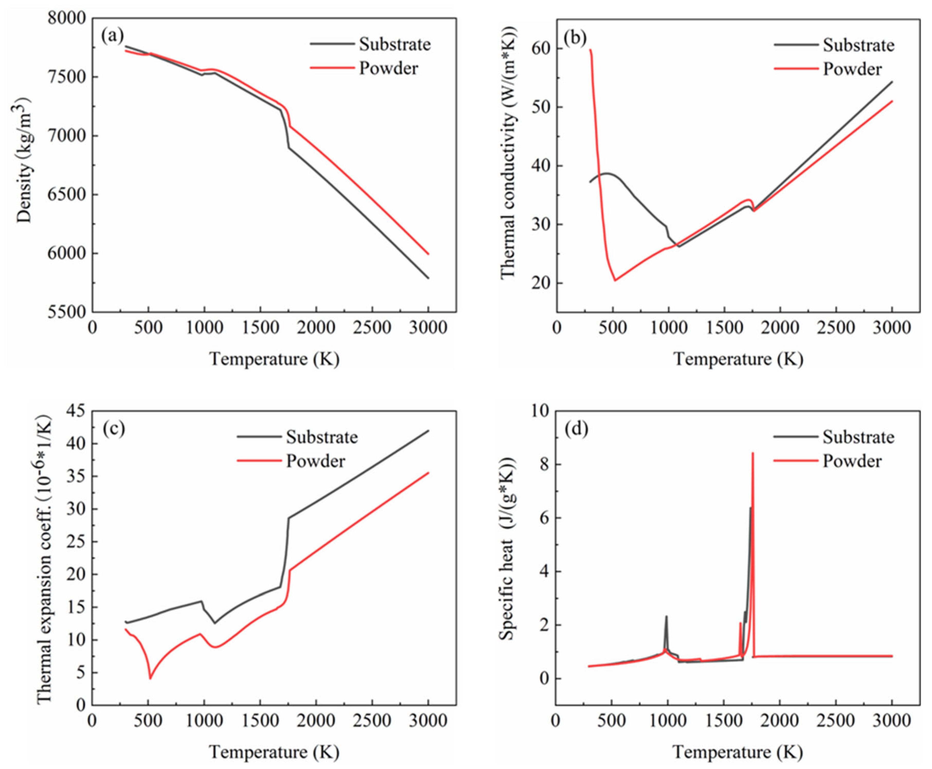
In this study, 27SiMn was used as the substrate, which is the main material of a domestic hydraulic cylinder. This substrate material encounters severe wear during its service in harsh environments. This inevitably causes defects, namely scratches, voids, cracks and shallow pits on the substrate surface. As a result, the service life of the component is reduced. The damage components were repaired with the use of different powders. The iron-based alloy powder with a particle size distribution of 20–53 µm was used as the cladding material, which has a good wear resistance, corrosion resistance and excellent machining properties. In addition, the fluid phase temperature and the expansion coefficient were similar to that of 27SiMn. Among the available different manufacturing techniques, the laser cladding process possessed higher efficiency, precise control of the layer thickness, superior bonding strength of repairing region with the substrate and widely applicable process. Hence, the powder and the substrate could form a firm metallurgy binding. The element mass fractions of the two materials are shown in Table 1. The CALPHAD phase diagram method was used to calculate the thermophysical properties of the material in this study. Zhang Linlang et al. [13] and Qiao Liang [14] compared the calculation result of the CALPHAD phase diagram method with the experimental measurement result and found a good correlation. The thermophysical properties of the substrate and powder were obtained through the calculation with the support of the CALPHAD phase diagram method, and the corresponding results are shown in Figure 1.

Table 1.
Elemental mass fractions of substrate and powder (wt%).
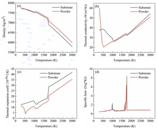
Figure 1.
Thermophysical properties of substrate and powder: (a) density; (b) thermal conductivity; (c) thermal expansion coefficient; (d) constant pressure heat capacity.
According to the Hagen–Rubens relational formula [15], the laser power absorptivity value of the substrate and powder can be obtained, as shown in Equation (1):
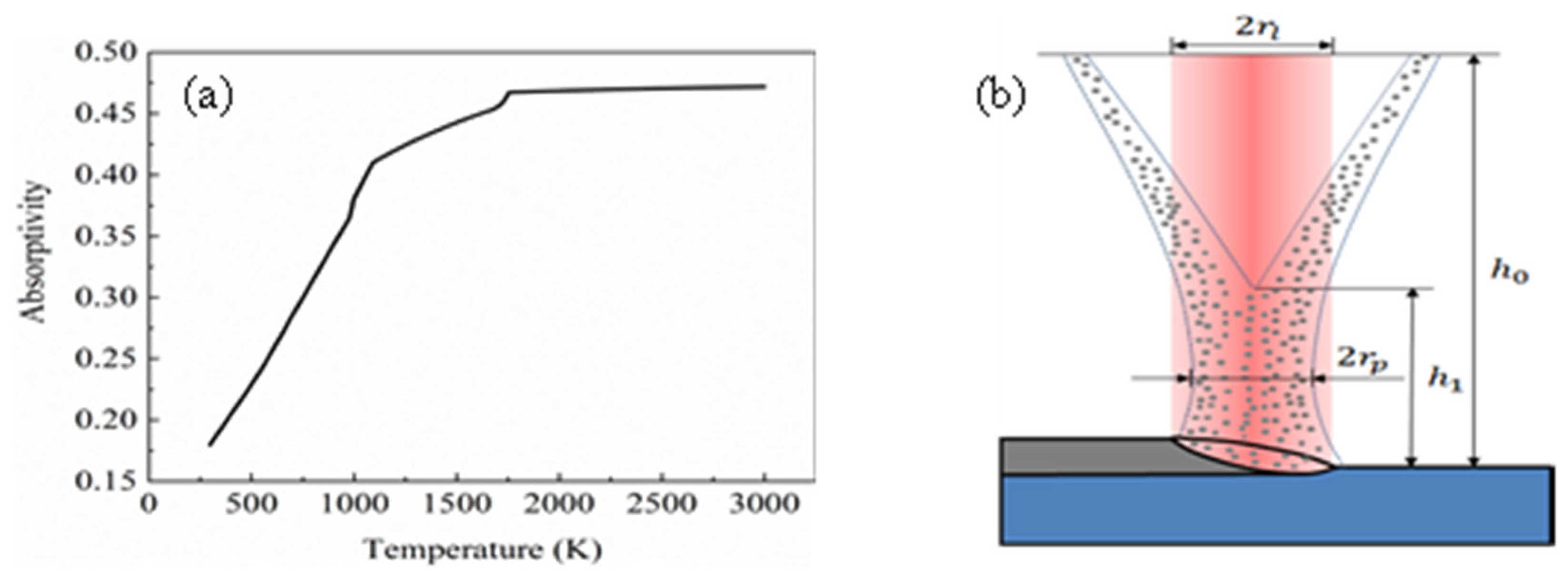
In Equation (1), c represents the speed of light in the vacuum, λ is the laser wavelength and R(T) represents the resistivity of the material, which is a function that changes with temperature. The laser absorption rate of the substrate is shown in Figure 2a. In order to simplify the calculation, a constant was selected for the laser absorptivity value of the powder. As the powder fell into the melt pool in a liquid form, βp was taken as 0.47. Figure 3 shows the determination of the powder flow radius relationship: (a) original image of the camera; (b) extracting data points on the contour; (c) fitting curve.
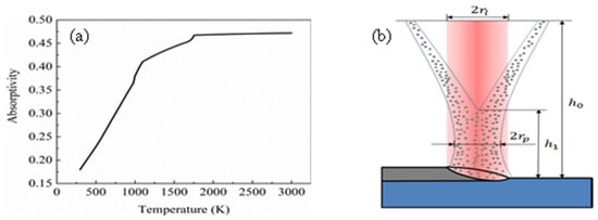
Figure 2.
(a) Laser absorption of the substrate; (b) schematic diagram of laser cladding.
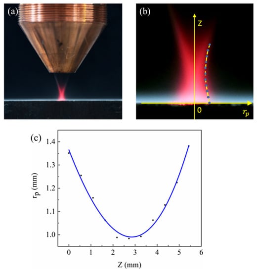
Figure 3.
Determination of the powder flow radius relationship: (a) original image of the camera; (b) extracting data points on the contour; (c) fitting curve.
2.1.2. Experimental Equipment
The experimental parameters of this study are shown in Table 2. A schematic diagram of laser classes is shown in Figure 2b. In the experiment, we explore the mutual coupling of laser and powder and determine the diameter of the powder flow profile, shown in Figure 4a. Here, the replacement light is a red light having a power of 5 W. An image recognition algorithm was used to extract the powder flow profile and select 11 data points. The establishment of the coordinate system is shown in Figure 4b, fitted to the expression of rp in the z direction, shown in Equation (2), with the fitted image as shown in Figure 4c.
Table 2.
Experimental Process parameters.
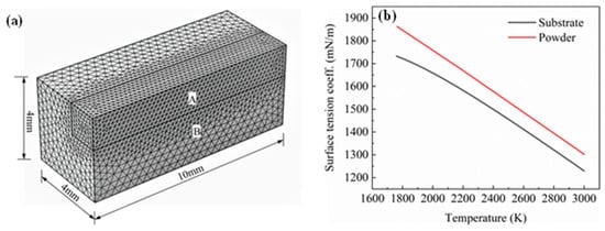
Figure 4.
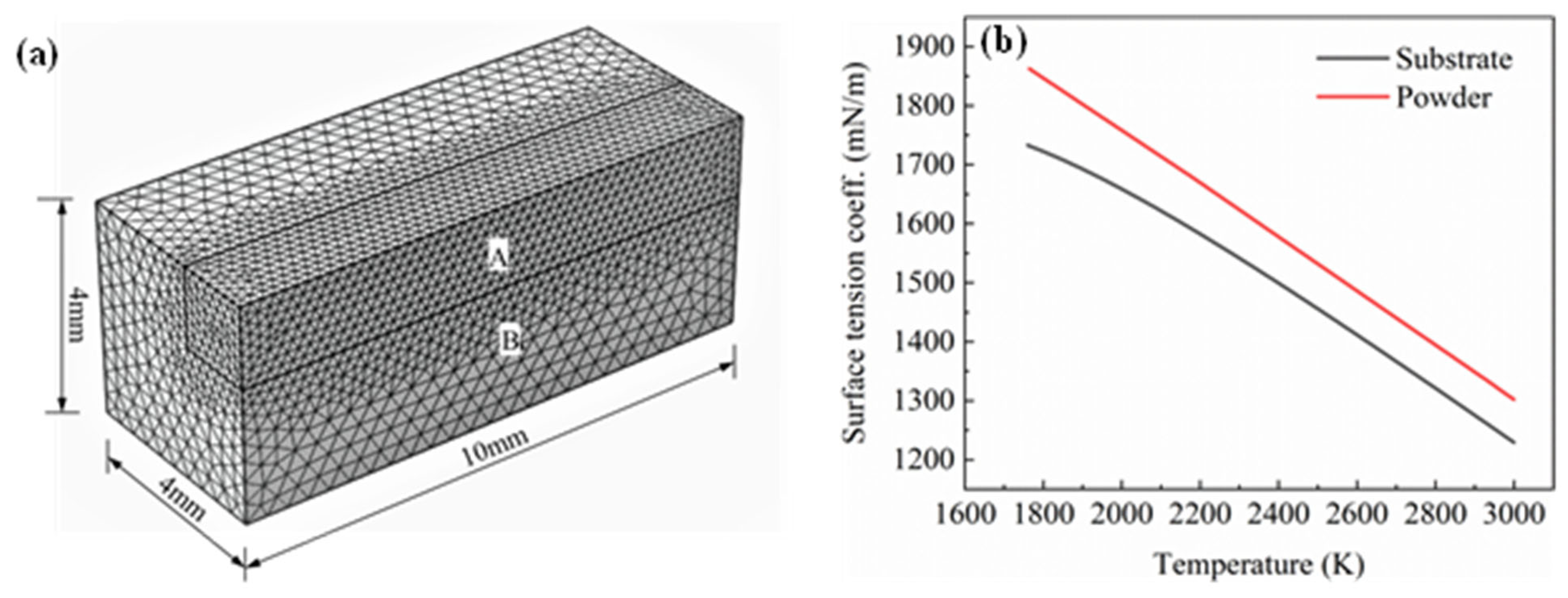
(a) Mesh division of the calculation area; (b) surface tension coefficient curve of the substrate and powder.
2.1.3. Process Parameters
This study adopted the method of orthogonal experiment. The process parameters of the experiment are shown in Table 3. Exp. 1, 2, 3 and 4 were used to explore the effects of different laser powers on the laser cladding processes; exp. 1, 5, 6 and 7 were used to explore the effects of different delivery rates on laser cladding processes [16]; exp. 1, 8, 9 and 10 were used to explore the effects of different scanning speed on the laser cladding process. The size of the substrate was 300 mm × 300 mm × 20 mm, and the room temperature was 298 K. Before the experiment, the powder was dried at 373 K for 2 h.
Table 3.
Process parameters of orthogonal experiment.
2.1.4. Experimental Detection
The cladding layers of the 10 groups of experiments were made into 10 sample blocks with a size of 10 mm × 10 mm × 15 mm, and the cross-section of those cladding layers was ground, polished, corroded and cleaned. The height and width of the cladding layer were observed under a metallographic microscope, and the microstructure was photographed with a scanning electron microscope (SEM).
2.2. Simulation
The use of numerical simulation in the field of engineering study is increasing. The content of the simulation is based on basic control equations, a set of reasonable assumptions, initial conditions and boundary conditions so that the numerical model is both efficient and realistic.
2.2.1. Assumptions
Appropriate assumptions can reduce the nonlinearity of the numerical model and enhance convergence. The basic assumptions in this study are as follows:
- The liquid metal in the melt pool is a Newtonian, incompressible and laminar fluid.
- The laser and powder flow comply with the Gaussian distribution, the powder flow profile is not affected by the powder feeding rate and the particles in the air do not block or collide with each other.
- The energy loss caused by evaporation is ignored.
- The mushy zone between the solid line and the liquid line of the melt pool is assumed to be an isotropic porous medium.
- The powder is a standard sphere and is heated evenly.
- The laser energy entering the melt pool through the reflection of powder particles is ignored.
2.2.2. Governing Equation
The mass conservation equation [17] is Equation (3):
The energy conservation equation is Equation (4):
In Equation (3), Smass represents the added powder mass; in Equation (4), the first term on the left is the transient heat transfer, the second term is the convective heat transfer, and the third term is the conduction heat transfer. The first term on the right is the heat source, the second term is the convection heat transfer with the outside and the third term is the surface heat radiation.
The momentum conservation equation (Navier–Stokes equation) is Equation (5):
In Equation (5), the left side represents the inertial force, the first term on the right represents the viscous force and pressure and the second term on the right represents the volume force of the liquid in the melt pool.
2.2.3. Initial Conditions
In order to save computational costs, a symmetric method was adopted to simplify the numerical model. A rectangular parallelepiped model with a size of 10 mm × 4 mm × 4 mm was established and divided into two calculation domains. The shape of calculation domain A was 10 mm × 1.5 mm × 1.5 mm. The mesh type was a free tetrahedral mesh. The computational domain A was the main area for melt pool calculation. The required accuracy was high. The maximum element size was 0.2 mm. Computational domain B was only used for heat transfer calculations, and the maximum element size was set to 0.4 mm, as shown in Figure 4a. The parameters of the model are as follows: initial temperature T0 = 298 K, external pressure P0 = 1 [atm], material convection velocity V0 = 0 m.s−1, initial displacement d0 = 0 m and the concentration of each element of the substrate material is set as the initial concentration.
2.3. Boundary Conditions
2.3.1. Thermal Boundary Conditions
The laser passed through the powder flow before reaching the substrate, and the powder flow caused the attenuation of the laser energy. Attenuation was caused by the combined effects of powder particles on laser energy absorption, diffraction, transmission, refraction and reflection [18]. At the same time, the powder absorbed the laser energy to increase its internal energy and change its physical state. Before reaching the substrate, the powder particles moved in a straight line at a uniform speed. The speed was the same as the vertical speed component of the powder-carrying gas at the outlet [19], and the speed direction was perpendicular to the surface of the substrate.
The concentration of powder flow “” in space is given in Equation (6) [20]:
The shading area of powder particles “” is shown in Equation (7):
The powder speed “” is shown in Equation (8), where θ is the angle between the outlet of the powder-carrying gas and the vertical direction.
The laser utilization rate “” is shown in Equation (9) [21]:
The average temperature of the powder before falling into the melt pool is shown in Equation (10):
The initial energy “” of the laser is shown in Equation (11):
The heat source “” formula added on the surface of the model is shown in Equation (12) [22]:
where is the liquid volume fraction, defined as Equation (13):
In Equation (13), is the ambient temperature; are the solidus and liquidus temperatures of the material, respectively.
When the temperature is between the solidus temperature and the liquidus temperature, the metal material is in a molten state, and the thermophysical properties of the material in this region are as shown in Equations (14)–(17).
When the temperature of the substrate rises, it will form heat convection “” with the surrounding air and generate heat radiation “” to the environment, as shown in Equations (18) and (19), respectively.
where is the convective heat transfer coefficient, which is 0.7, ε is surface emissivity and σ is Stepan Boltzmann’s constant, the value of which is .
2.3.2. Fluid Boundary Conditions
The volume force “” received by the liquid in the melt pool in Equation (5) can be expanded to Equation (20):
In the formula, the first term on the right represents gravity. The second term on the right represents thermal buoyancy, α is the thermal expansion coefficient of the mixed material in the melt pool, and the direction is vertically upward. The third term on the right represents the momentum dissipation of the porous media layer between the solid phase and the liquid phase on the liquid metal in the melt pool, where K0 takes the larger value, 106 kg·(m−3·s−1); in order to avoid division by zero errors, m takes the smaller value, 10−4 [23].
On the surface of the melt pool, the liquid metal was subject to surface tension. The surface tension coefficient is a physical quantity that changes with temperature and concentration. In this study, the influence of concentration changes on surface tension was not considered. The curve of the surface tension coefficient with temperature was obtained based on the CALPHAD phase diagram method, as shown in Figure 4b. It can be seen from Figure 4b that the higher the temperature, the smaller the surface tension coefficient, that is, the surface tension temperature coefficient is negative. Since the temperature decreased from the centre of the melt pool to the edge, the surface tension also decreased from the centre of the melt pool to the edge, forming a surface tension gradient. The liquid flowed from the direction of low surface tension to high tension, thereby driving the transmission of mass. This phenomenon is called the Marangoni effect.
As a dimensionless number, the Marangoni number “” is proportional to the ratio of the surface tension divided by the viscous force, indicating the degree of the Marangoni effect on the flow of liquid metal.
where dγ/dT is the temperature coefficient of surface tension, L is the characteristic length, μ is the dynamic viscosity and ∆T is the maximum temperature difference in the melt pool.
The force on the surface “ of the melt pool is as follows (22):
where γ is the surface tension coefficient, nm is the normal vector of the melt pool surface, κ is the average curvature of the melt pool surface and ∇t is the tangential guide number operator of the melt pool surface.
2.3.3. Mass Transfer Boundary Conditions
In the numerical simulation, the adding process of powder was resolved into volume change and element change. The volume change was characterized by the dynamic grid algorithm, and the element change was represented by the matter flux equation. The transmission speed of the element and the velocity field were set in a coupling relationship.
The material flux “” [24] on the surface of the melt pool is shown in Equation (23):
During the cladding process, the powder falls into the melt pool and fully mixes with the substrate under the action of the Marangoni effect. Therefore, the thermophysical properties “” of the liquid metal in the melt pool are determined by the properties of the substrate and the powder.
In Equation (24) [25], P represents the thermophysical properties of the model, including density, thermal conductivity, dynamic viscosity, constant pressure heat capacity, surface tension coefficient, etc., represent the thermophysical properties of the powder and the substrate, respectively, and represents the degree of powder mixing in the melt pool and is calculated by Equation (25) [25]:
where represents the iron element concentration of the model in the transient calculation process, and represent the initial iron element concentration in the substrate and powders, respectively, and the unit is .
2.3.4. Mesh Boundary Conditions
The algorithms currently used to represent volume changes mainly include life and death units [12,26], level sets [27] and the Arbitrary Lagrangian–Eulerian (ALE) moving mesh approach [24]. Given that the forming accuracy of the life and death unit algorithm is low, the level set algorithm is complex and difficult to set. While the moving grid algorithm is simple to set up and can form a more accurate interface, the dynamic grid algorithm is used to characterize the formation of the cladding layer. The moving speed of the melt pool surface is mainly affected by the addition of powder and the flow of liquid metal in the melt pool; therefore, in the ALE moving mesh approach, the moving speed “” of the melt pool surface [28] is
In Equation (26), Vs is the moving speed of the melt pool surface, Vp is the moving speed of the melt pool surface due to powder addition, v is the flow velocity of the liquid metal on the melt pool surface and nm represents the unit normal vector of the melt pool surface.
The moving speed “” of the melt pool surface due to powder addition is
In Equation (27), ηp is the powder utilization rate, ρp is the density of the powder, rp0 is the radius of the powder flow on the substrate and zm is the unit vector in the z direction.
3. Results and Discussion
3.1. The Results of Numerical Calculation
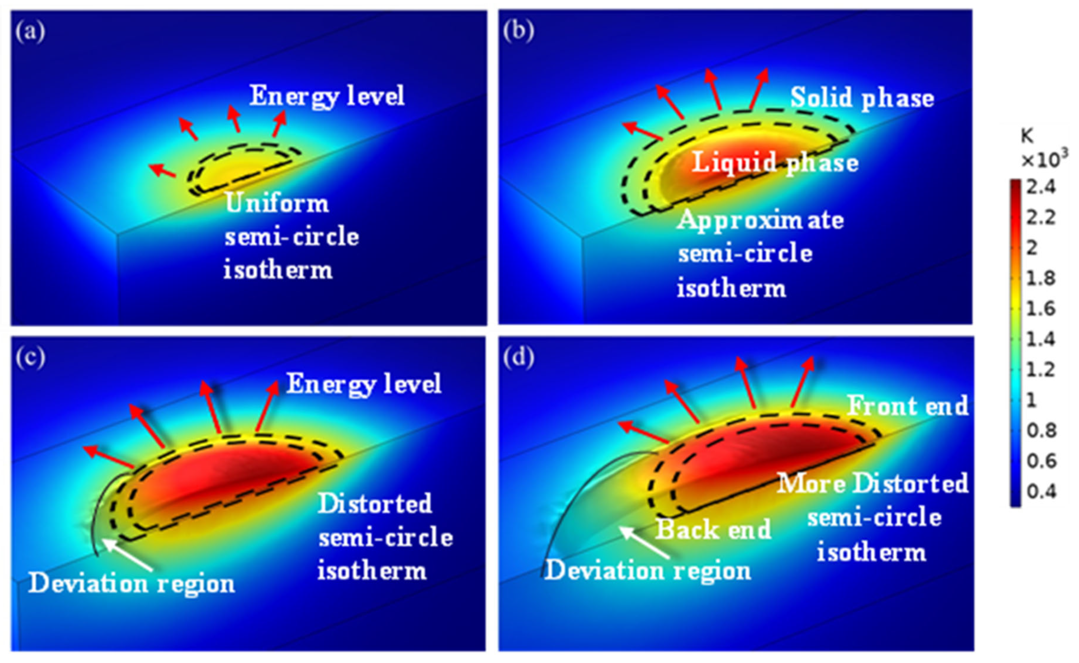
A heat source was applied on the upper surface of the model. The initial conditions and boundary conditions are given in Section 2.2.3 and Section 2.3, and the temperature at different times was obtained. The simulated temperature distribution profile at different time intervals of the laser beam interaction with the substrate surface is shown in Figure 5. Two semi-circle dotted curves represent the solid and liquid phase separation. The outside curve shows the solid phase limit, whereas the inside curve denotes the liquid phase limit. The direction of the arrow shows that the energy was transferred from the centre to the outside. The length of the arrow reveals the energy level at that particular point. The direction of the arrow is around the hemispherical curve, as the transfer of energy has taken place in a direction perpendicular to an isothermal vector. The sum of (1) the energy absorbed by the powder and the substrate and (2) that reflected by the powder and substrate are equivalent to the total energy involved during the laser cladding process. The sudden increases in the temperature of the 27SiMn substrate (red colour in Figure 5) revealed that the substrate has the capability of a high absorption rate. The semi-circular shape uniformly increased and then diverged in shape within the four stages. These stages took place from the start of the interaction of the laser beam to the movement of the laser beam to the next stage. These variations occurred due to the supply of thermal energy as well as heat transfer from the melt pool to the atmosphere. A detailed discussion of each stage is carried out below.

Figure 5.
Temperature distribution at different moments in the simulation results of exp. 1: (a) 30 ms; (b) 50 ms; (c) 100 ms; (d) 150 ms.
The interaction of the laser beam with the cladding region within the duration of 20 ms is shown in Figure 5a. In this initial stage of laser cladding, the laser started heating the substrate; the melt pool was not formed at this time, and the temperature was reduced from the centre to the surrounding area. One of the assumptions made was the isotopic property that resulted in the circular shape of the temperature distribution at this initial stage. The arrow length was very small, which confirmed the lower energy level during the initial stage compared to the remaining stages. The temperature of the cladding region rose to 1600 K (yellow colour) at the time of 30 ms from the laser beam interaction with the substrate. However, the size of the circle was very small, and the isotherm coverage area was less. This shape deviated continuously as the time of interaction increased.
The isotherm distribution of the first 50 ms duration of the laser beam interaction with the cladding region is shown in Figure 5b. In this laser cladding stage, the significant size of the melt pool was observed, and the temperature reached up to 2200 K (light red colour). However, the size of the highest temperature distribution was very much less, but higher than that of the temperature stage at 30 ms. The temperature loss to the surrounding atmosphere was low, which was confirmed by maintaining the isotherm as an approximate semi-circle and not stretching more. Small deviations in the semi-circle shape confirmed the interaction with the surrounding atmosphere medium. The arrow length was larger compared with that of the 30 ms of the isotherm profile due to an increase in the energy level. The isotherm size was larger than that of the 30 ms profile, which revealed the increase in the coverage region and melting of a large amount that led to the forming of the cladding region accordingly.
The interaction of the laser beam with the cladding region within the duration of 100 ms is shown in Figure 5c. The local temperature was higher than the material liquid phase line temperature, which increased the size of the melt pool. In this laser cladding third stage, the deviation of the semi-circle was observed as the heat energy lost to the surrounding atmosphere space. The maximum temperature of 2400 K (dark red colour) was reached at the centre of the melt pool region. The arrow length was larger, which confirmed the large energy level compared to the remaining stages. However, the size of the circle was large, and the isotherm coverage area was large. This shape deviated continuously as the time of interaction increased. As the powder continued to accumulate in the melt pool, the cladded surface began to deform.
The isotherm distribution of the first 150 ms duration of the laser beam interaction with the cladding region is shown in Figure 5d. In this laser cladding stage, the maximum temperature reached up to 2400 K (light red colour). The size of the highest temperature distribution was maximum compared with the remaining three stages. The temperature loss to the surrounding atmosphere was also large, which was confirmed by the larger deviation of the semi-circle and stretching in one direction. These large deviations in the semi-circle shape confirmed the interaction with the surrounding atmosphere medium. The arrow length was larger when compared with that of the 100 ms of the isotherm profile due to an increase in the energy level. The isotherm size was larger than that of the 100 ms profile, which revealed the increase in the coverage region and melting of a large amount that led to the forming of the cladding region accordingly. As the laser beam moved in the scanning direction, the temperature gradient in the melt pool exhibited a high front end and a low back end. As a result, the circular isotherm region was present at the highest temperature region (front end) and the deviation of the semi-circle appeared at the back end. The presence of the energy at the back end dissipated to the surrounding atmosphere and the semi-circle was elongated.
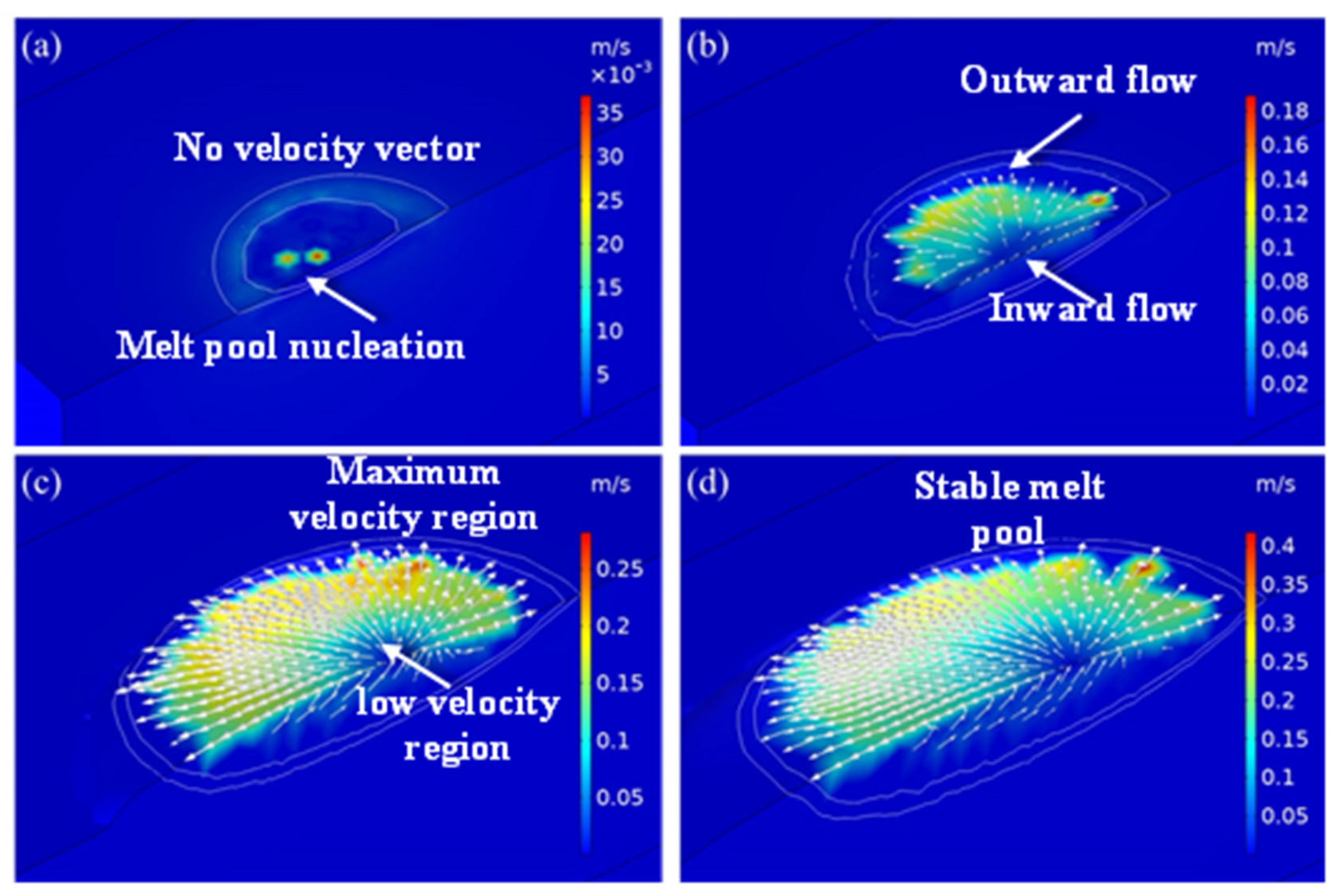
The velocity profile of the laser-cladded region at different time frames is shown in Figure 6. The flow of the liquid metal in the melt pool at different times was varied and is discussed in detail in this section. Significantly different velocity profiles were found at various time intervals, such as the initial stage, melt pool expansion stage, wide–shallow melt pool stage and stable stage. The white line segment represents the liquid and solid phase lines of the model, and the arrow represents the flow direction of the liquid metal in the melt pool. The thermal energy was supplied to the cladded region and was transferred to the material through conduction and Marangoni convection. The heat flow was outward from the melt pool surface, as the temperature coefficient, surface tension and temperature distribution had negative values. As the temperature increased, the volume of the melt pool expanded, and the liquid metal in the melt pool flowed under the action of surface tension, gravity and thermal buoyancy. Moreover, the negative temperature coefficient of surface tension caused the liquid metal on the melt pool surface to flow from the centre to the edge, under the influence of the Marangoni effect. Due to the existence of gravity and thermal buoyancy, liquid metal flowed into the bottom of the melt pool along the solidification interface and then rose to the surface of the melt pool, forming an eddy current from inside to outside. Under the action of the eddy current, a wide and shallow melt pool was formed. As the melt pool moved, the temperature rose, and the shape of the melt pool gradually changed from a semi-circle to an ellipsoid. The flow velocity in the melt pool accelerated until it became stable. The velocity direction was consistent with the research results of Acharya et al. [29], and the value was of the same order of magnitude.
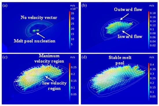
Figure 6.
Velocity distribution at different moments in the simulation results of exp. 1: (a) 30 ms; (b) 50 ms; (c) 100 ms; (d) 150 ms.
The distribution of the velocity profile of liquid metal at the initial stage is shown in Figure 6a. In the initial stage of the melt pool formation, the liquid metal in the melt pool did not flow, up to the time of 30 ms. As a result, there was no velocity line of liquid metal present in the cladded region. In this stage, the melt pool started to form even though the temperature of the input thermal energy was higher than the melting point of the material due to heat conduction to the substrate. Here, heat conduction was more dominant than other forms of heat transfer. In addition, the melt pool and flow velocity were nucleated, which can be observed in Figure 6a. This growth in the melt pool increased with the continuous supply of laser energy.
The velocity profile of the laser-cladded region at the 50 ms time domain is shown in Figure 6b. The flow of the liquid metal in the melt pool is clearly visible in Figure 6b. Most of the direction of the flow vector was toward the outside of the melt pool, as the value of the temperature coefficient, surface tension and temperature distribution were negative. As a result, the melt pool expanded outside from the centre of the melt pool. A few of the arrows were found in the inverted direction, because, due to the existence of gravity and thermal buoyancy, liquid metal flowed at the bottom of the melt pool along the solidification interface. These arrows rose to the surface of the melt pool from inside to outside due to the formation of an eddy current. This process continued until the whole size of the melt pool formation increased.
Figure 6c shows the distribution of the velocity profile of liquid metal at the wide melt pool stage. In this stage of melt pool formation, the liquid metal in the melt pool flows varied from 0.05 to 0.25 m·s−1 over the region. The maximum velocity of 0.25 m·s−1 was observed at the periphery of the melt pool, whereas a velocity of 0.05 m·s−1 was formed at the bottom region of the melt pool. This type of distribution was formed at the time of 100 ms. The liquid metal flow was much lower at the centre of the melt pool region due to the attainment of high temperature. Under the action of an eddy current, a wide and stable melt pool was formed. This growth in the melt pool increased with the continuous supply of laser energy. As the melt pool moved, the temperature rose, and the shape of the melt pool gradually changed from a semi-circle to an ellipsoid. The flow velocity profile of the laser-cladded region at the 150 ms time domain is shown in Figure 6d. The flow velocity in the liquid metal in the melt pool flows accelerated until it became stable. The maximum velocity of 0.4 m·s−1 was achieved in most of the region of the periphery of the melt pool. This value was 60% higher than that of the velocity at a 100 ms time frame. This velocity direction was consistent with the research results of Acharya et al. [29], and the value was of the same order of magnitude. The flow rate increased due to the dominant Marangoni convection.
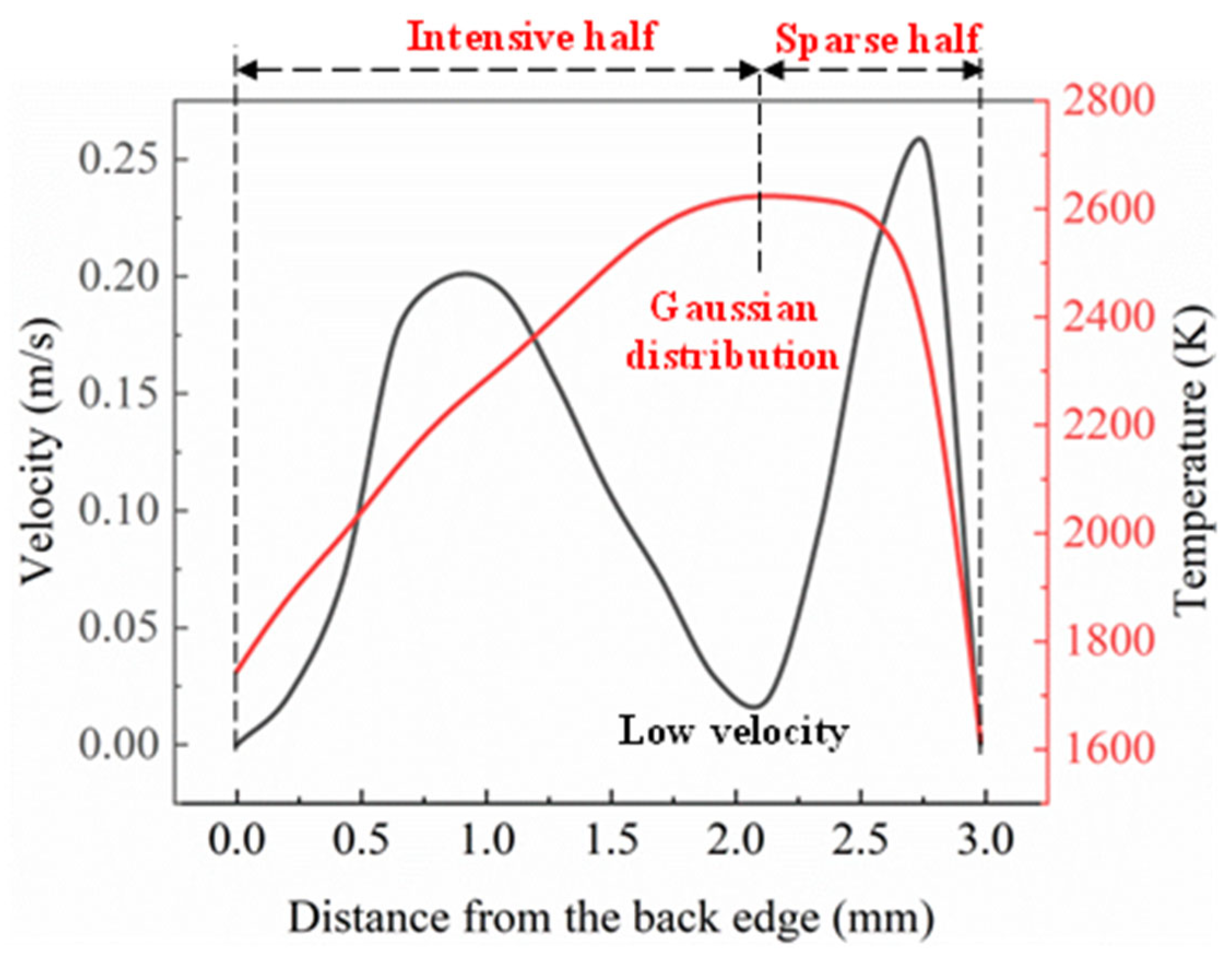
The temperature and velocity distribution curves of the melt pool surface along the scanning velocity direction at the time of 100 ms are shown in Figure 7. It can be seen from Figure 6 that the flow rate of the liquid metal on the melt pool surface presents a hump distribution, the flow rate at the bottom of the melt pool is lower than that on the melt pool surface, and the maximum velocity in the melt pool is 0.25 m·s−1. The Marangoni effect played an important role in promoting the flow of liquid metal in the melt pool. The greater the temperature gradient, the more intense was the Marangoni effect, and thus, the greater the acceleration. The flow at the bottom of the melt pool was affected by the process of cellular crystal forming, resulting in momentum loss. The liquid metal at the bottom of the pool flowed upward under the action of thermal buoyancy. The velocity at the centre of the melt pool surface was close to that at the bottom of the pool because the thermal buoyancy was not sufficient enough to produce a large flow acceleration.
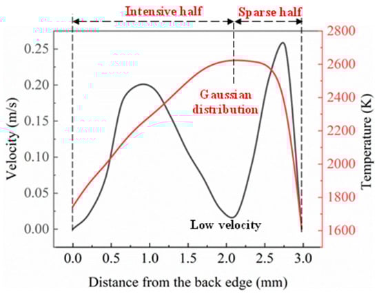
Figure 7.
Temperature and velocity distribution curve in the direction of scanning speed on the surface of the melt pool.
The velocity of the liquid metal flow at the maximum temperature point (the laser spot centre) was lower than that of the other position. Figure 7 reveals that the flow rate first increased to 0.2 m·s−1 and started to decrease toward the centre of the laser beam (maximum temperature point). The relation between the surface tension with the temperature was negative at the high-temperature condition. Hence, this type of flow behaviour was induced due to the negative value of the surface tension temperature coefficient.
The molten liquid flowed from a lower surface tension position to a higher surface tension location. The temperature distribution path at 100 ms revealed the formation of a Gaussian distribution profile (refer to red colour curve in Figure 7) due to the Gaussian distribution profile around the centre of the laser beam input heat energy [30]. In the first half, it was observed that the distribution of temperature was intensive, whereas the second half possessed a sparse distribution of temperature. This distribution was well-suited for the cladding process, as the irradiation occurred within the region of the coaxial powder deposition and substrate surface. The temperature decreased in the second half (sparse region) and reached the lowest temperature at a point of 3 mm from the back edge.
3.2. Comparison of External Dimensions
The geometry of the cladded surface was influenced by the flow of non-isothermal energy in the melt pool region. Comparing the profile size of the cladded layer was the most intuitive and simplest method to verify the accuracy of the model. The simulation result was validated with the experimental results, and the deviation of the dimension was identified to study the error of the simulation model. Figure 8 shows the dimensions of the cross-section obtained using different parameters such as power, scanning speed and powder feed rate through the experimental work as well as the simulation model.
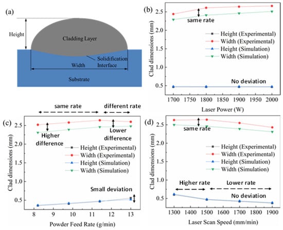
Figure 8.
Numerical prediction and experimental results of the dimensions of the deposited single tracks for (a) schematic cross-section; (b) varying laser power; (c) varying powder feeding rate; (d) varying laser scanning speed.
The width and height of the cladded layer are schematically represented in Figure 8a. It can be seen from Figure 8b that, when only the laser power was changed by maintaining a constant scanning speed and powder feed rate, the height of the cladded layer hardly changes. However, the width of the cladded layer increased with the increase in the laser power from 1700 W to 2000 W. The reason was that, with the laser power becoming larger, the energy irradiated to the surface of the substrate increased, the temperature at the centre of the melt pool increased and the width of the melt pool became larger. While the height of the cladded layer was mainly related to the amount of powder falling into the melt pool, under the premise of a constant powder feeding rate, the height of the centre of the cladded layer remained unchanged.
Figure 8c shows the dimension of the cladded layer at varying powder feed rates with a constant power and scanning speed condition. The larger powder feeding rate led to a smaller laser attenuation rate. The powder feed rate was increased from 8 to 13 g·min−1; it was found that the height of the cladded layer decreased significantly as the powder feeding rate decreased both in the experiment and simulation. However, as it can be seen from Figure 8c, the height of the cladded layer obtained by the experimental measurement is slightly greater than the simulation model at the powder feed rate of 12 to 13 g·min−1. In the remaining region, the variation between the experimental and simulation height values was very negligible. The width of the cladded layer increased with the increase in the powder feed rate. The rate of increase of width was slightly less at the powder feed rate of 11.5 to 13 g·min−1 during the experimental measurement, whereas the simulation model gave the same rate of increase in width throughout the process. The difference between the experimental and simulation width values was around 0.5 mm. This difference was maintained from an 8 to 11.5 g·min−1 powder feed rate; afterwards (11.5 to 13 g·min−1), a decrease in the difference was observed.
The effect of scanning speed on the geometry of the cladded layer was studied by maintaining a constant power and powder feed rate. The height of the cladded layer hardly changed. Figure 8d shows the experimental and simulation results of varying scanning speeds from 1300 mm·min−1 to 1900 mm·min−1. The width and height of the cladded layer were analysed. The increase in scanning speed led to a decrease in the instantaneous energy density and instantaneous powder concentration on the substrate, which caused the formation of a narrow and long melt pool. When the scanning speed was too high, the material on the surface of the substrate could not be melted sufficiently, forming a cladded layer with poor bonding, or even no cladded layer. When the scanning speed was too low, a disordered accumulation of powder was caused. It can be observed from Figure 8d that the height of the cladded layer decreased with the increase in the scanning speed. The height of the cladded layer significantly decreased between the scanning speed of 1300 mm·min−1 and 1500 mm·min−1. However, the decreasing rate was reduced when the laser beam was moved at the scanning speed of 1500 mm·min−1 to 1900 mm·min−1. A similar study was carried out on the measurement of the width of the cladded layer. The experimental measurement gave a higher value than the simulation model, around 0.5 mm. The width of the cladded layer decreased with the increase in the scanning speed from 1300 mm·min−1 to 1900 mm·min−1, similar to the height of the cladded layer. However, the decrease rate was the same throughout the above-specified scanning speed range. The comparisons between the simulation and experimental results are listed in Table 4.
Table 4.
Comparation between the simulation and the experimentation.
Based on the overall observation from Figure 8, the height of the layer obtained by the simulation was greater than the experimental measurement, and the width was slightly smaller. In this study, in order to reduce the degree of nonlinearity of the model, the dynamic viscosity of the liquid metal in the melt pool was limited, resulting in the deterioration of fluidity. Hence, the width of the molten coating layer of the simulation was smaller. During the laser cladding experiment, the powder was ejected from the nozzle, which caused some powder loss, and this phenomenon was ignored in the simulation; hence, the high degree of the simulation was slightly higher than the height measured by the experiment. The maximum error of the experimentally measured shape and simulation calculation was 8%, indicating the rationality of the three-dimensional laser-cladded model. The error obtained from this experiment was at a reasonable level when compared with the studies available in the open literature [7].
3.3. Energy Distribution
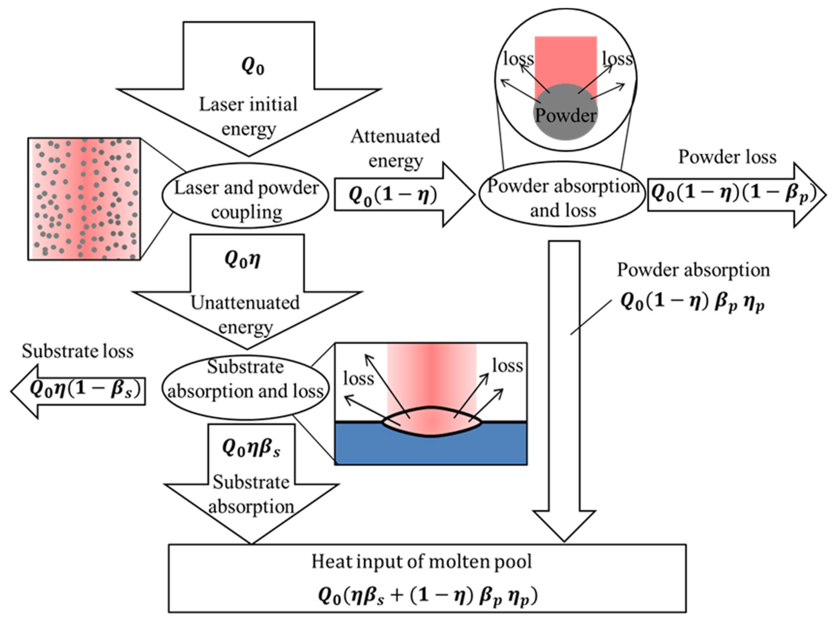
The energy transfer process of laser cladding is shown in Figure 9. The initial energy output by the laser reached the surface of the substrate after the attenuation of the powder. However, not all the attenuated energy was absorbed by the substrate material. The substrate has a certain absorption rate of laser energy, which is related to the resistivity of the material and the laser wavelength. During the experiment, the laser wavelength was constant. The material resistivity is a physical property related to temperature, and the laser absorption rate of the substrate is shown in Figure 2a. Part of the energy attenuated by the powder was absorbed by the powder, and the rest was released to the outside world through refraction, scattering and reflection. Only the powder falling into the melt pool can play a role in the formation of the cladded layer; so, the powder utilization rate represents the ratio of the amount of powder falling into the melt pool to the total amount of powder.

Figure 9.
Energy distribution process in the cladding process.
The laser energy absorbed according to Figure 9 is given by Equation (28):
According to Equation (9), the laser utilization is calculated. According to Figure 2a, it is known that the laser absorption rate of the substrate is , so , that is, 10% of the laser energy in exp. 1 is used to heat the substrate to form a melt pool.
During the transmission of laser energy, the dissipative energy “” is shown in Equation (29):
When powder utilization , is calculated, that is, at least 53% of the laser energy in the cladding process is released into the environment.
The thermal input “” in the melt pool is shown in Equation (30):
After analysis and calculation, it was found that the energy for heating the substrate to form the fuse pool only accounts for 10% of the laser output energy; about 53% of the energy is consumed. The research results of Gedda et al. [18] have evolved this conclusion.
3.4. Solidification Characteristics
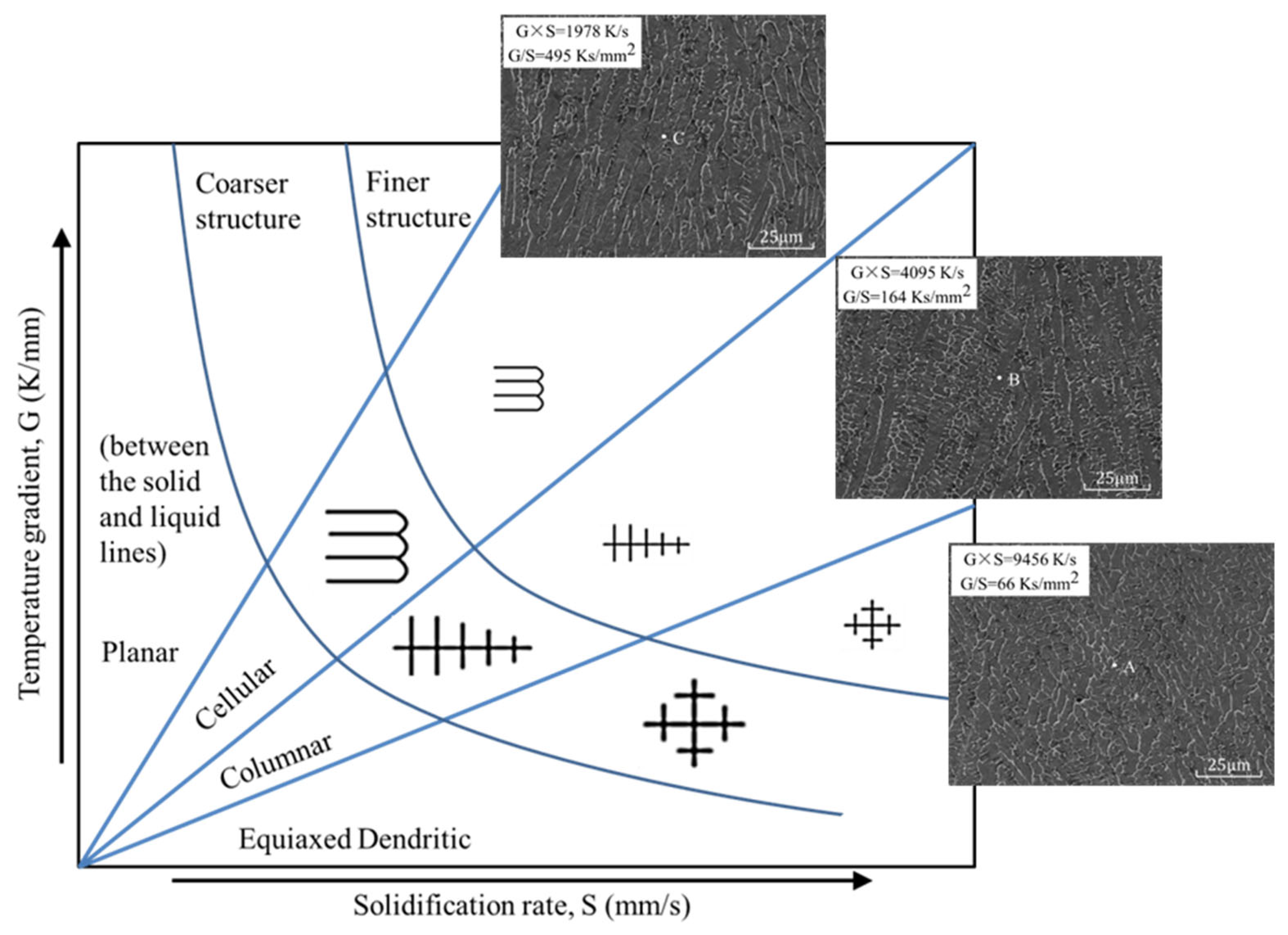
The laser cladding process needed to undergo rapid heating and cooling. In this process, the temperature gradient (G) and the solidification speed (S) on the solidification interface were two crucial parameters. Changes in G and S directly affected the microstructure of the cladded layer and then affected the surface quality of the layer. The influence of G and S on the microstructure is shown in Figure 10 [19,20]. The correlation of the melt pool with the corresponding microstructure is analysed in detail at the end of this section. G×S is defined as the cooling rate, which directly determines the size of the microstructure grains. The faster the cooling rate, the finer the microstructure grains. The value of G/S determines the microstructure morphology. As G/S gradually increases, the microstructure morphology changes from cellular to equiaxed dendritic.

Figure 10.
The influence of G and S on the microstructure.
The directions of G and S are perpendicular to the solidification interface, and their respective expressions are [31]
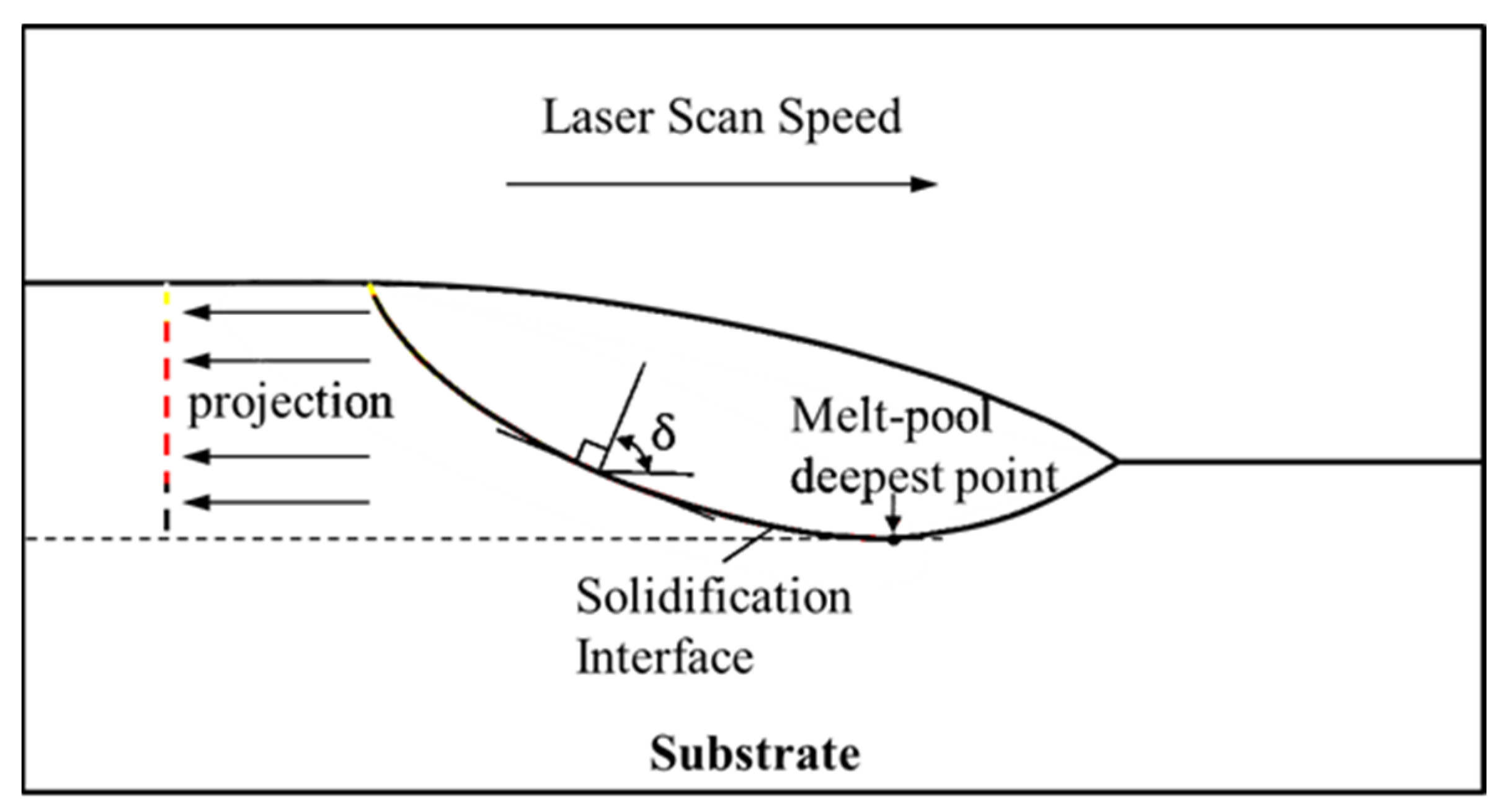
In Equation (31), δ represents the angle between the normal vector of the solidification interface and the scanning speed direction on the vertical plane.
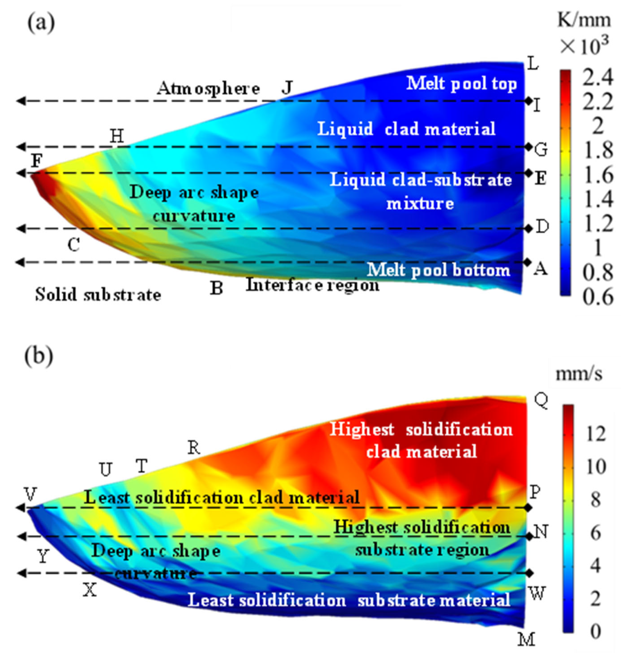
The minimum angle at the top of the cladded layer was almost 0°, and the maximum angle at the bottom was 90°. Hence, the solidification speed was the largest at the top and was close to the scanning speed, and the minimum at the bottom was 0 m·s−1. The projection diagram of the solidification interface on the melt pool symmetry is shown in Figure 11. The simulation result when the time was 200 ms in exp. 1 was selected, and the size of G and S on the solidification interface was projected on a two-dimensional plane, as shown in Figure 12. The morphology of the cladded layer with respect to the temperature gradient and solidification rate is discussed in this section. The distribution of the G value in the melt pool region transformed from a thin arc shape to a deep arc shape [32]. The distribution of the G value in the melt pool region initially started from a thin arc shape and transformed into a wave shape due to the changes in a boundary at the bottom arc region. With the further addition of the heat input through the laser energy, the wave shape was changed to a full arc shape. Solidification started from the interface region to the top of the surface. The interface region between the two phases, liquid and solid, is clearly observed in Figure 12a. The melt pool top and the bottom region at the centre are denoted as L and A, respectively. The penetration of laser energy in the substrate is revealed by the presence of a curved bottom shape melt pool below the top surface of the substrate.
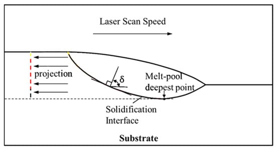
Figure 11.
Projection of the solidification interface on the melt pool symmetry.

Figure 12.
(a) The temperature gradient G and (b) the solidification rate S in the calculation results.
The G value at the location along the points A, D, E, G, I and L were very low, in the range of 0.6 × 10³ to 1 × 10³ K·mm−1. It showed that the difference in the temperature at the centre plane was minimal compared with the remaining location of the melt pool region. A higher difference in temperature was observed at the edges of the melt pool. The highest temperature was observed at point F, which was the extreme point of the melt pool region. However, the maximum temperature was observed in the range of 2 × 10³ to 2.4 × 10³ K·mm−1, spread across the points C to F. Moreover, this highest temperature difference was located in the substrate region rather than the cladded region, which confirmed the complete melting of the clad powder. In addition, a few temperature differences between points F and H are observed in Figure 12a, showing that slight microstructure changes occurred away from the centre of the cladded region.
In the region H to J, a difference in the temperature was formed with the temperature gradient range of 1.2 × 10³ to 1.4 × 10³ K·mm−1. This value was smaller than the peak temperature gradient value and slightly higher than the minimum temperature gradient value. This temperature gradient spread in the triangular shape of HJB, as base regions were present at the cladded region and apex reign was present at the substrate region. Figure 12a reveals that the temperature difference uniformly increased from the centre to the edges. The rate of increase was small from the centre to the vertical section BJ and then drastically increased up to point F. In more than half of the melt pool, the temperature difference was in the range of 0.6 × 10³ to 1 × 10³ K·mm−1 (blue colour in Figure 12a). In the remaining melt pool region, the values were 1 × 10³ to 2.4 × 10³ K·mm−1. The region of 1.2 × 10³ to 1.4 × 10³ K·mm−1 (sky blue colour) covered most of the area in the remaining region of the melt pool. The peak temperature difference region of 2.2 × 10³ to 2.4 × 10³ K·mm−1 was the smallest region of the melt pool. This distribution showed that the microstructure was uniformly varied within the melt pool region.
Figure 12b shows the solidification rate of the melt pool of the cladded and substrate regions. A significant difference was observed in the solidification rate within the melt pool region. The solidification of the cladded material was higher compared with the substrate material in the region of PVQ. The maximum solidification rate of 12 mm·s−1 was observed at the topmost point of the melt pool region. This maximum solidification rate was distributed in the form of a triangle as the PQR. It revealed that the cladded powder was melted well and solidified faster than other regions by the rapid heating and cooling process of the laser cladding technique. In addition, away from the cladded centre region, the solidification rate was reduced from 12 mm·s−1 to 8 mm·s−1. This 8 mm·s−1 solidification was observed at the region of VR that is located at the edge of the melt pool region. The cladded region was solidified with a solidification rate of 8 mm·s−1 to 12 mm·s−1. However, the substrate region in the melt pool part reached the maximum solidification rate of 8 mm·s−1. Moreover, in most parts of the melt pool region on the substrate side, the solidification rate was in the range of 4 mm·s−1 to 6 mm·s−1 (sky blue colour in Figure 12b). Nearer to the substrate, the solidification rate had the lowest value of 2 mm·s−1.
Figure 12b reveals that the bottom half of the melt pool solidified more slowly than the upper half of the melt pool. As a result, a different microstructure was formed at the centre line QPNM, which is analysed with the corresponding SEM images in the next section. The solidification rate changed significantly in the radial direction, whereas in the horizontal direction, its value was nearly constant. This trend was more severe in the bottom half than in the upper half. Three different segregations were observed in the bottom half in the radial direction. The rectangular region VPNY had the highest solidification rate in the bottom-half region of the melt pool. Further, NYXW possessed a moderate solidification rate in this bottom-half region. The lowest solidification rate occurred at the region of WXM, which was on the nearest surface to the un-melted substrate material. In the upper region of the melt pool, two different solidification segments were observed. The vertical region of the centre part of the melt pool region at the upper region possessed the same solidification region, in contrast to the bottom.
The regions of the highest solidification rate of 12 mm·s−1 and the lowest solidification rate of 2 mm·s−1 are clearly visible in Figure 12b. However, the transformation of the solidification rate from 4 mm·s−1 to 10 mm·s−1 took place together. As a result, the intermediate region appeared with a mixture of sky blue, green and yellow colours. It confirmed that the microstructure significantly changed due to this variation in the solidification rate. Specifically, the solidification rate of 6 mm·s−1 to 8 mm·s−1 (a green colour region in Figure 12b) was not clearly visible, showing the drastic change in the solidification rate in the 100 µm region.
Figure 12a,b show that the solidification rate and the temperature differences varied throughout the melt pool region. The region ADEGIL in Figure 12a has the same temperature difference value, but the solidification rate varied significantly from a minimum value of 2 mm·s−1 to a maximum value of 12 mm·s−1. This variation occurred throughout the melt pool region. In addition, the highest solidification rate (PQR) was observed at the lowest temperature gradient region (LJGI) and vice versa. The least variation between the solidification rate and temperature difference was found at edge UT in Figure 12b. In addition, the variation in the vertical direction from M to Q occurred as seen in Figure 12b; the horizontal direction variation along line EF is observed in Figure 12a. This analysis gave a significant outline to the variation in the solidification rate and temperature differences in the melt pool region.
The surface tension was small, as the temperature difference at the surface of the melt pool region was small (JL region in Figure 12a). However, the surface tension was higher at the edge (HFC line in Figure 12a) of the melt pool due to the presence of a large temperature difference. In addition, these surfaces were located far away from the laser source; hence, it was not possible to observe the laser energy. The heat transfer through the convection mode at the bottom (AB line in Figure 12a) of the melt pool was small. At the same time, this value was large at the sides (HJBC region in Figure 12a).
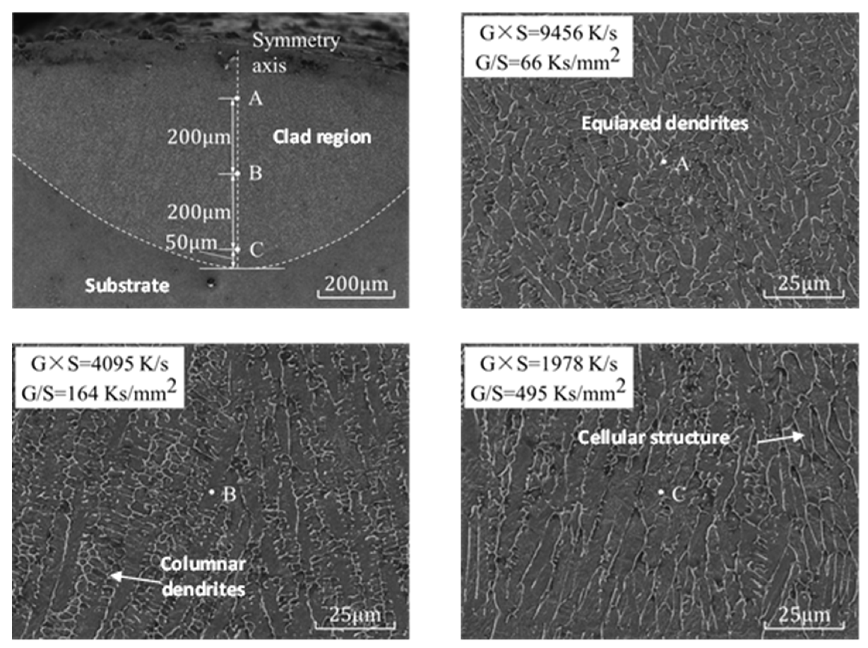
The sample of exp. 1 was selected for line cutting, grinding and etching, and the microstructure in the SEM was photographed, as shown in Figure 13. From the top to the bottom of the molten coating symmetry, three measuring points, A, B and C, were selected from the bottom isometric. From point A to C, G × S decreased from 9456 K·s−1 to 1978 K·s−1, and the microstructure grain gradually became large [33].

Figure 13.
Melt pool at laser clad region and microstructure of points A, B and C of the cladding layer in exp. no. 1.
G/S increased from 66 Ks·mm−2 to 495 Ks·mm−2, and the microstructure transformed from equiaxed dendritic (point A) to cellular (point B), and further grew into a columnar dendritic structure in point C. The experimental results are highly consistent with the simulation results, and the model has high reliability.
4. Conclusions
The laser cladding process was carried out on the 27SiMn material, and the corresponding simulation was modelled by setting a reasonable hypothetical condition, initial condition, boundary condition and parameters. The following conclusions were derived based on the experimental and simulation results:
- The simulation model presented in this study gave an accuracy of 92% by comparing 10 sets of experimental results.
- The maximum laser energy that can be utilized at the melt pool region in the laser cladding process was found as 10%, which gives the alert for future work to find the new process window for enhancing the heat utilization.
- This research work shows the correlation of the temperature gradient and solidification rate of the simulation model with the microstructure of the experimental laser-cladded region.
- The specific microstructure, such as equiaxed dendritic, cellular and columnar dendritic, can be cultivated to fulfil the requirement for a specific property by following this research output.
- The new path of research nucleates to reduce the energy wastage to the environment, as this research work found that 53% of laser energy was dispelled into the environment as heat loss during the laser cladding process.
- The multiplication value of the temperature gradient and solidification rate was negatively correlated with the microstructure size.
Author Contributions
K.M.: Conceptualization, Methodology, Software, Validation, Investigation, Writing—Original Draft. Y.C.: Conceptualization, Writing—Review and Editing, Visualization, Supervision, Funding Acquisition. N.J.: Methodology, Validation, Investigation, Writing—Review and Editing. J.Z.: Conceptualization, Methodology, Software. Y.W.: Conceptualization, Software, Visualization. W.Y.: Conceptualization, Methodology, Investigation. All authors have read and agreed to the published version of the manuscript.
Funding
This work was supported by the National Key Research and Development Program (2023YFE0201600), Fundamental Research Funds for the Central Universities (2021ZDPY0223) and a Project Funded by the Priority Academic Program Development of Jiangsu Higher Education Institutions.
Data Availability Statement
The experimental datasets obtained from this research work and the analysed results during the current study are available from the corresponding author on reasonable request.
Conflicts of Interest
The authors declare that they have no known competing financial interests or personal relationships that could have appeared to influence the work reported in this paper.
References
- Wang, H. Study progress of laser surface modification of metal materials and laser rapid prototyping of high-performance metal parts. Acta Aeronaut. Sin. 2002, 23, 473–478. [Google Scholar]
- Shi, Q.; Wang, Z.; Shao, Y. Application of laser cladding technology in coal mine machinery. China Equip. Eng. 2021, 185–186. [Google Scholar]
- Hu, C.; Xu, J.; Yang, J. Application of laser cladding surface strengthening in runner chamber of hydropower station. Hydropower New Energy 2021, 35, 50–52. [Google Scholar]
- Jiang, Y.; Cheng, Y.; Zhang, X.; Yang, J.; Yang, X.; Cheng, Z. Simulation and experimental investigations on the effect of Marangoni convection on thermal field during laser cladding process. Optik 2020, 203, 164044. [Google Scholar] [CrossRef]
- Sun, Z.; Guo, W.; Li, L. Numerical modelling of heat transfer, mass transport and microstructure formation in a high deposition rate laser directed energy deposition process. Addit. Manuf. 2020, 33, 101175. [Google Scholar] [CrossRef]
- Deng, Z.; Liu, D.; Liu, G.; Liu, J.; Li, C.; Li, S.; Chen, T. Numerical simulation study on the formation mechanism of hydroxyapatite-silver gradient bioactive ceramic coatings under wide-band laser cladding. Opt. Laser Technol. 2023, 163, 109412. [Google Scholar] [CrossRef]
- Wang, C.; Zhou, J.; Zhang, T.; Meng, X.; Li, P.; Huang, S. Numerical simulation and solidification characteristics for laser cladding of Inconel 718. Opt. Laser Technol. 2022, 149, 107843. [Google Scholar] [CrossRef]
- Zhang, Q.; Xu, P.; Zha, G.; Ouyang, Z.; He, D. Numerical simulations of temperature and stress field of Fe-Mn-Si-Cr-Ni shape memory alloy coating synthesized by laser cladding. Optik 2021, 242, 167079. [Google Scholar] [CrossRef]
- Chai, Q.; Zhang, H.; Fang, C.; Qiu, X.; Xing, Y. Numerical and experimental investigation into temperature field and profile of Stellite6 formed by ultrasonic vibration-assisted laser cladding. J. Manuf. Process. 2023, 85, 80–89. [Google Scholar] [CrossRef]
- Wang, S.; Shi, T.; Fu, G. Dilution rate and single-pass morphology analysis of high-speed cladding Cr50Ni alloy with laser powder feeding. Surf. Technol. 2020, 49, 311–318. [Google Scholar]
- Wei, H.L.; Elmer, J.W.; DebRoy, T. Origin of grain orientation during solidification of an aluminum alloy. Acta Mater. 2016, 115, 123–131. [Google Scholar] [CrossRef]
- Gao, W.; Zhao, S.; Wang, Y.; Zhang, Z.; Liu, F.; Lin, X. Numerical simulation of thermal field and Fe-based coating doped Ti. Int. J. Heat Mass Transf. 2016, 92, 83–90. [Google Scholar] [CrossRef]
- Zhang, L.; Xiong, C. Study on Material Forming Training Teaching Based on JMatPro Simulation Analysis Software. J. Sci. Technol. Econ. Guide 2020, 28, 108–109. [Google Scholar]
- Qiao, L. Study on Empirical Model and JMatPro Software to Calculate Martensite Onset Temperature. Hot Work. Technol. 2017, 46, 94–96+103. [Google Scholar]
- Xie, J.; Kar, A.; Rothenflue, J.A.; Latham, W.P. Temperature-dependent absorptivity and cutting capability of CO2, Nd:YAG and chemical oxygen–iodine lasers. J. Laser Appl. 1997, 9, 77–85. [Google Scholar] [CrossRef]
- Jeyaprakash, N.; Yang, C.H.; Tseng, S.P. Wear Tribo-performances of laser cladding Colmonoy-6 and Stellite-6 Micron layers on stainless steel 304 using Yb: YAG disk laser. Met. Mater. Int. 2021, 27, 1540–1553. [Google Scholar] [CrossRef]
- Wen, S.; Shin, Y.-C. Modeling of transport phenomena in direct laser deposition of metal matrix composite. Int. J. Heat Mass Transf. 2011, 54, 5319–5326. [Google Scholar] [CrossRef]
- Gedda, H.; Powell, J.; Wahlström, G.; Li, W.B.; Engström, H.; Magnusson, C. Energy redistribution during CO2 laser cladding. J. Laser Appl. 2002, 14, 78–82. [Google Scholar] [CrossRef]
- Fu, Y.; Martin, B.; Loredo, A.; Vannes, A.B.; Li, J. Velocity Distribution of the Powder Particles in Laser Cladding. Chin. J. Lasers B 2002, 11, 469–474. [Google Scholar]
- Gan, Z. Study on Heat and Mass Transport in Laser Additive Manufacturing of Superalloys; University of Chinese Academy of Sciences: Beijing, China, 2017. [Google Scholar]
- Chen, L.; Zhao, Y.; Song, B.; Yu, T.; Liu, Z. Modeling and simulation of 3D geometry prediction and dynamic solidification behavior of Fe-based coatings by laser cladding. Opt. Laser Technol. 2021, 139, 107009. [Google Scholar] [CrossRef]
- Chew, Y.; Pang JH, L.; Bi, G.; Song, B. Thermo-mechanical model for simulating laser cladding induced residual stresses with single and multiple clad beads. J. Mater. Process. Technol. 2015, 224, 89–101. [Google Scholar] [CrossRef]
- Bahrami, A.; Helenbrook, B.T.; Valentine, D.T.; Aidun, D.K. Fluid flow and mixing in linear GTA welding of dissimilar ferrous alloys. Int. J. Heat Mass Transf. 2016, 93, 729–741. [Google Scholar] [CrossRef]
- Gan, Z.; Liu, H.; Li, S.; He, X.; Yu, G. Modeling of thermal behavior and mass transport in multi-layer laser additive manufacturing of Ni-based alloy on cast iron. Int. J. Heat Mass Transf. 2017, 111, 709–722. [Google Scholar] [CrossRef]
- Li, C.; Yu, Z.B.; Gao, J.X.; Zhao, J.Y.; Han, X. Numerical simulation and experimental study on the evolution of multi-field coupling in laser cladding process by disk lasers. Weld. World 2019, 63, 925–945. [Google Scholar] [CrossRef]
- Fallah, V.; Amoorezaei, M.; Provatas, N.; Corbin, S.F.; Khajepour, A. Phase-field simulation of solidification morphology in laser powder deposition of Ti–Nb alloys. Acta Mater. 2012, 60, 1633–1646. [Google Scholar] [CrossRef]
- He, X.; Mazumder, J. Transport phenomena during direct metal deposition. J. Appl. Phys. 2007, 101, 53113. [Google Scholar] [CrossRef]
- Song, J.; Chew, Y.; Bi, G.; Yao, X.; Zhang, B.; Bai, J.; Moon, S.K. Numerical and experimental study of laser aided additive manufacturing for melt-pool profile and grain orientation analysis. Mater. Des. 2018, 137, 286–297. [Google Scholar] [CrossRef]
- Acharya, R.; Bansal, R.; Gambone, J.J.; Das, S. A Coupled Thermal, Fluid Flow, and Solidification Model for the Processing of Single-Crystal Alloy CMSX-4 Through Scanning Laser Epitaxy for Turbine Engine Hot-Section Component Repair (Part I). Metall. Mater. Trans. B 2014, 45, 2247–2261. [Google Scholar] [CrossRef]
- Jeyaprakash, N.; Yang, C.H.; Susila, P.; Karuppasamy, S.S. Laser Cladding of NiCrMoFeNbTa Particles on Inconel 625 Alloy: Microstructure and Corrosion Resistance. Trans. Indian Inst. Met. 2022, 76, 599–612. [Google Scholar] [CrossRef]
- Zhao, J.; Wang, G.; Wang, X.; Luo, S.; Wang, L.; Rong, Y. Multicomponent multiphase modeling of dissimilar laser cladding process with high-speed steel on medium carbon steel. Int. J. Heat Mass Transf. 2020, 148, 118990. [Google Scholar] [CrossRef]
- Tian, H.; Chen, X.; Yan, Z.; Zhi, X.; Yang, Q.; Yuan, Z. Finite-element simulation of melt pool geometry and dilution ratio during laser cladding. Appl. Phys. A 2019, 125, 485. [Google Scholar] [CrossRef]
- Li, C.; Liu, C.; Li, S.; Zhang, Z.; Zeng, M.; Wang, F.; Wang, J.; Guo, Y. Numerical Simulation of Thermal Evolution and Solidification Behavior of Laser Cladding AlSiTiNi Composite Coatings. Coatings 2019, 9, 391. [Google Scholar] [CrossRef]


Disclaimer/Publisher’s Note: The statements, opinions and data contained in all publications are solely those of the individual author(s) and contributor(s) and not of MDPI and/or the editor(s). MDPI and/or the editor(s) disclaim responsibility for any injury to people or property resulting from any ideas, methods, instructions or products referred to in the content. |
© 2023 by the authors. Licensee MDPI, Basel, Switzerland. This article is an open access article distributed under the terms and conditions of the Creative Commons Attribution (CC BY) license (https://creativecommons.org/licenses/by/4.0/).