A Metallurgical Dynamics-Based Method for Production State Characterization and End-Point Time Prediction of Basic Oxygen Furnace Steelmaking

Abstract

Basic Oxygen Furnace (BOF) steelmaking is an important way for steel production. Correctly recognizing different blowing periods and abnormal refining states is significant to ensure normal production process, while accurately predicting the end-point time helps to increase the first-time qualification rate of molten steel. Since the decarburization products CO and CO₂ are the main compositions of off-gas, information of off-gas is explored for BOF steelmaking control. However, the problem is that most of the existing research directly gave the proportions of CO and CO₂ as model input but barely considered the variation information of off-gas to describe the production state. At the same time, the off-gas information can be expected to recognize the last blowing period and predict the end-point time earlier than the existing methods that are based on sub-lance or furnace flame image, but little literature makes an attempt. Therefore, this work proposes a new method based on functional data analysis (FDA) and phase plane (PP), defined as FDA-PP, to describe and predict the BOF steelmaking process from the metallurgical dynamics viewpoint. This method extracts the total proportion of CO and CO₂ and its first-order derivative as dynamics features of steelmaking process via FDA, which indicate the reaction velocity and acceleration of decarburization reaction, and describes the evolution of dynamics features via PP. Then, the FDA-PP method extracts the features of phase trajectories for production state recognition and end-point time prediction. Experiments on a real production dataset demonstrate that the FDA-PP method has higher production state recognition accuracy than the classical phase space, SVM, and BP methods, which is 87.78% for blowing periods of normal batches, 90.94% for splashing anomaly, and 81.29% for drying anomaly, respectively. At the same time, the FDA-PP method decreases the mean relative prediction error (MRE) of the end-point time prediction for abnormal batches by about 10% compared with the SVM and BP methods.

1. Introduction

Basic Oxygen Furnace (BOF) steelmaking is important in the iron and steel industry, through which over 70% of crude steel is refined all over the world [1]. A successful BOF steelmaking process should have a normal production process, accurate end-point time, and stable product quality. In reality, the process control often relies on the experience and skill of operators, so that the abnormal production state, insufficient refining time, and unqualified molten steel sometimes appear, which would threaten production safety and increase energy and resource consumption. Therefore, lots of models [2,3,4] are studied to recognize different blowing periods and abnormal refining states in order to optimize process parameters and ensure normal production process, as well as to predict the end-point time or oxygen blowing volume (dividing the oxygen blowing volume by the oxygen flow can obtain the end-point time) in order to increase the first-time qualification rate of molten steel and avoid re-blowing operation.

With the trend of intelligent manufacturing in the iron and steel industry [5,6], data-based methods [7,8,9] are developing for the above targets relying on the abundant production data, including: the sub-lance measurements, the furnace flame image, and the off-gas. Han Min et al. [10] and He Fei et al. [11] employed the adaptive-network-based fuzzy inference system (ANFIS) and the back-propagation neural network (BP) respectively to predict the oxygen blowing volume, where the model inputs were the metal’s carbon content and temperature measured by TSC sub-lance. But the sub-lance measurements are unavailable for the production state recognition. Meanwhile, the sub-lance detection is always carried out within the last 1 min, and needs to suspend the process operations, which breaks the production rhythm. The furnace flame image supports both the production state characterization and the end-point prediction and can be collected without production interruption. Prof. Li Ailian’s team studied the ResNet network [12] and the improved DenseNet network [13] to recognize different blowing periods relying on the furnace flame image. Wen Hongyuan [14] extracted the features of the furnace flame image and used the multiple linear regression (MLR) model and the BP model to predict the end-point time. But due to that, the end-point time prediction relied on the feature mutation of the furnace flame image which occurred very late, the time margin given by the existing model was only 20~40 s [14], too small to optimize operation parameters and adjust the steel quality.

The off-gas also supports both the production state characterization and the end-point prediction. The industry has been exploring the use of off-gas information for process control. Mats Bramming [15] built a multiway partial least squares (MPLS) model using the off-gas information and other process data to explain and predict the splashing anomaly. Our previous works [16] proposed a Mahalanobis distance-based functional derivative support vector data description (MD-FDSVDD) model to identify the splashing anomaly from the amplitude variations of off-gas. Compared with the furnace flame image, the off-gas data are sensitive to the change of decarburization rate since the decarburization products CO and CO₂ are the main compositions of off-gas. Thus, the off-gas data can be expected to predict the ending time with a larger time margin as the decarburization rate changes when the last blowing period begins.

However, for the existing research, most of the data-based models directly gave the amplitude of off-gas composition as input to a model and then obtained the output of the production state. This end-to-end calculation ignored part of the metallurgical dynamics features of BOF steelmaking, i.e., the variation information of decarburization rate, leading to a hard determination of production state with similar amplitude of off-gas composition (i.e., similar decarburization rate). As the BOF steelmaking process contains complex multi-phase physicochemical reactions, lots of operation parameters will affect the decarburization rate [17,18,19,20], and different parameters have diverse effects. On this basis, employing the variation information of off-gas composition is significant to explain how the decarburization rate is going to change with the influence of operation parameters, so that to provide an accurate description of the production state.

Therefore, this work proposes a new data-based method from the viewpoint of metallurgical dynamics to characterize the steelmaking production state and predict the end-point time. This method is based on the theories of functional data analysis (FDA) and phase plane (PP), defined as FDA-PP. The FDA-PP method firstly smooths the discrete sequences of the total proportion of CO and CO₂ in the off-gas via FDA to obtain their continuous functions and first-order derivative functions. Then, the phase plane is constructed by the fitting functions and derivative functions. The phase trajectory characterizes the decarburization rate as well as the influence of the operation parameters on the decarburization rate, describing the evolution of the production state. Next, a boundary that indicates a stable production state is estimated on the phase plane via support vector data description (SVDD) to recognize different blowing periods and abnormal production state. When the phase trajectory indicates that the last blowing period begins, the future phase trajectory is predicted via case-based reasoning (CBR), further estimating the end-point time.

Based on the above, the proposed FDA-PP method has four aspects of contributions and advantages. First, the FDA-PP method takes comprehensive consideration of the decarburization rate as well as its variation trend and establishes a metallurgical dynamics-based model for production state characterization. Second, this work is an attempt that using the off-gas data to characterize different blowing periods and predict the end-point time. Although the evolution of off-gas compositions was used to successfully recognize the splashing and drying anomalies, little literature tried to use it to identify different blowing periods. At the same time, to the best of our knowledge, the off-gas information hasn’t been used for the end-point time/oxygen blowing volume prediction. Third, the FDA-PP method can be expected to predict the end-point time with 2~4 min in advance since the prediction is implemented at the beginning of the last blowing period. Fourth, based on the FDA, problems of irregular data such as uneven refining durations, different sampling frequencies, noise, and missing values, can be settled, and the evolution characteristics of the time-series data can be retained in the smoothed curves.

The remainder of this article is organized as follows: Section 2 gives an overview of BOF steelmaking and illustrates the connection between the metallurgical dynamics features with the phase plane; Section 3 describes the procedures to realize the FDA-PP method; Section 4 verifies the FDA-PP method and compares it with some commonly used methods; Section 5 makes a conclusion.

2. Problem Statement

This section first introduces the BOF steelmaking process and then analyzes the connection between the metallurgical dynamics of BOF steelmaking with the phase plane.

2.1. Overview of BOF Steelmaking

BOF steelmaking is an important way for steel production and its primary purposes are to remove the carbon content of molten steel from 4~5% to around 0.04~0.06% and increase the temperature from around 1250 °C to around 1680 °C [21]. Figure 1 is a schematic representation of the blowing process. The molten iron and the steel scrap are the main materials. The oxygen blowing from the top provides an oxidizing condition, while the nitrogen or argon blowing from the bottom acts as a stir. The auxiliary materials are added to help control the steel quality. Through controlling the oxygen lance height, the bottom blowing flow, and the weight of auxiliary materials, the molten steel is obtained [20].

The main reactions during the blowing process are the decarburization reactions, where the carbon of molten iron is oxidized by the oxygen blowing through $\left[\mathrm{C}\right]+\left[\mathrm{O}\right]=\mathrm{CO}\uparrow$ and $\left[\mathrm{C}\right]+2\left[\mathrm{O}\right]={\mathrm{CO}}_2\uparrow$. Since carbon monoxide and carbon dioxide are released with the off-gas, the off-gas compositions reflect the decarburization rate of the steelmaking process [20]. According to the change of decarburization rate, the oxygen blowing can be separated to three blowing periods [22]: the first blowing period, the main blowing period, and the end blowing period, as shown in Figure 2a. Correspondingly, the change of the total proportion of CO and CO₂ in the off-gas also shows three periods, as can be seen in Figure 2b. In the first blowing period, the total proportion of CO and CO₂ in the off-gas gradually rises with increasing decarburization reaction. In the main blowing period, the decarburization rate keeps on a high value, so the total proportion of CO and CO₂ holds on a large percentage. In the last blowing period, the total proportion of CO and CO₂ decreases as the decarburization rate decreases.

The splashing and drying anomalies usually happen in the main blowing period and their influences on the total proportion of CO and CO₂ are shown in Figure 2c,d. When the splashing anomaly happens, the total proportion of CO and CO₂ drops first and then rises up. When the drying anomaly happens, the trends of CO and CO₂ increase first and then decrease, showing opposite evolutions to the splashing batch.

2.2. Metallurgical Dynamics and Phase Plane of the BOF Steelmaking

The phase plane is a method that can describe the evolution of a system’s dynamics state [23,24], usually plotted with the first-order derivative and the second-order derivative. In this work, we take the decarburization reaction as the objective and use the phase plane to describe the evolution of the production state during the steelmaking process.

Since the total proportion of CO and CO₂ in the off-gas reflects the reaction velocity of the decarburization reaction in the metal pool [20], its first-order derivative indicates the reaction acceleration of the decarburization reaction, which is extracted to construct a phase plane in order to describe the dynamics evolution of decarburization reaction, i.e., the production state of BOF steelmaking. Figure 3a is the phase plane of the normal steelmaking process. We can see the phase trajectory begins at the origin point, develops clockwise from the first quadrant, holds on in a narrow region at the transverse axis, and goes back to the origin point from the fourth quadrant. The evolution of the phase trajectory is accordant to the dynamic characteristics of BOF steelmaking. In detail:

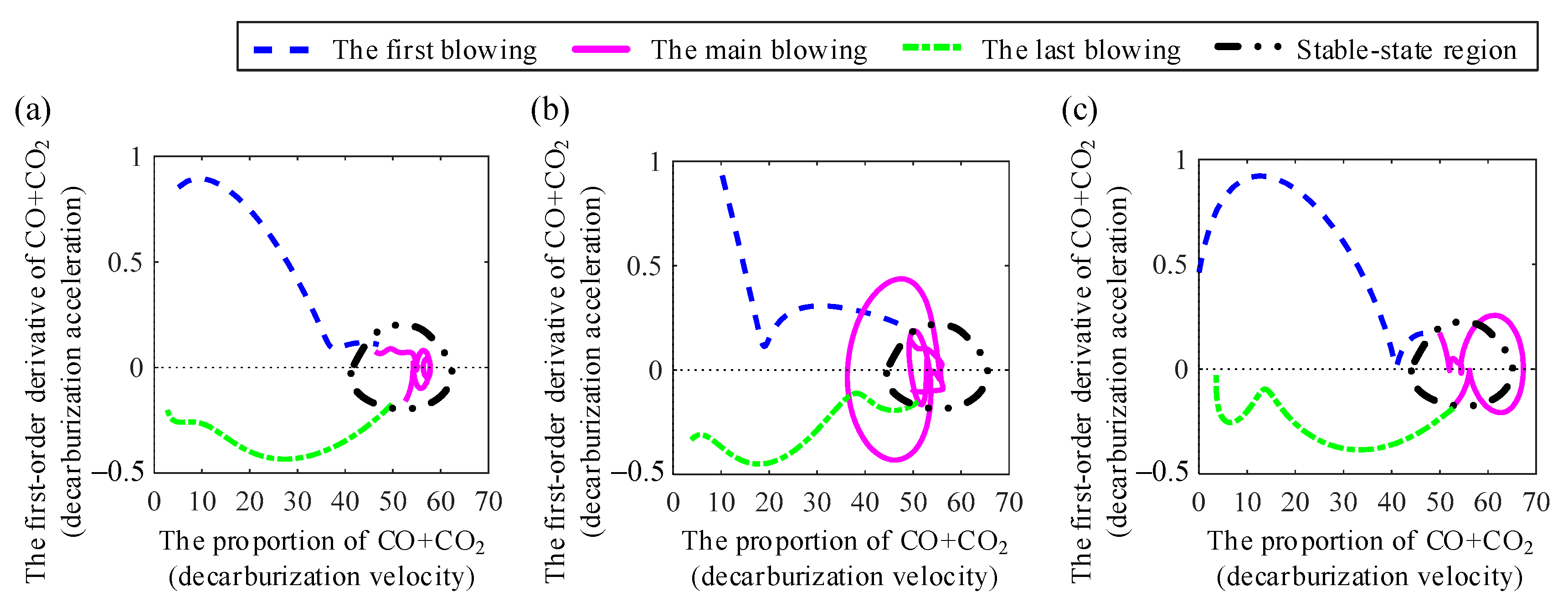
• Within the first blowing period, the phase trajectory shows increasing decarburization velocity and decreasing decarburization acceleration. The reason is that in the beginning, the silicon and manganese in the metal pool are preferentially oxidized and the carbon is following. With the silicon and manganese gradually consumed, the decarburization rate is enhanced. At the same time, as the carbon-oxygen reactions gradually reach their balances, the decarburization acceleration decreases.
• Within the main blowing period, the phase trajectory shows a stable state with the max decarburization velocity and nearly zero decarburization acceleration. The reason is that when the carbon concentration is high enough so that the transportation rate of oxygen limits the decarburization rate; thus, under a certain oxygen blowing, the decarburization reactions reach their balance condition and remain at their highest reaction velocities.
• Within the last blowing period, the phase trajectory shows decreasing decarburization velocity and a first decreasing then slightly increasing decarburization acceleration. The reason is that when the carbon concentration of the metal pool is too low so that the transportation rate of carbon limits the decarburization rate, with the unchanged oxygen blowing, the decarburization acceleration would be negative and decrease rapidly, further leading to decreasing decarburization velocity. With the carbon concentration tending to be zero, the decarburization acceleration and velocity are close to zero.

Figure 3b,c are the phase planes with splashing and drying anomalies respectively. Because of the abnormal fluidity of the slag emulsion [22], the splashing anomaly happens when the off-gas hardly traverses the slag emulsion and accumulates in the converter, whereas the drying anomaly happens when the off-gas rapidly traverses the slag and is released from the converter. Corresponding to this mechanism, when the splashing anomaly happens, the accumulated oxidation products CO and CO₂ prevent the decarburization reaction, so the decarburization velocity and acceleration rapidly decrease; after the off-gas erupts, the decarburization reaction recovers, so the decarburization velocity and acceleration rapidly increase. On this basis, the phase trajectory of the splashing anomaly exceeds the region of the stable state, develops clockwise from the fourth quadrant to the first quadrant, and finally goes back to the stable-state region. As for the drying anomaly, the decarburization reaction is promoted first because of the rapidly released off-gas and then returns to the normal level, so the phase trajectory exceeds the stable-state region and develops clockwise from the first quadrant to the fourth quadrant before returning to the stable-state region.

Based on these evolution features of the phase trajectory, different blowing periods and abnormal production states can be recognized.

3. Method Description

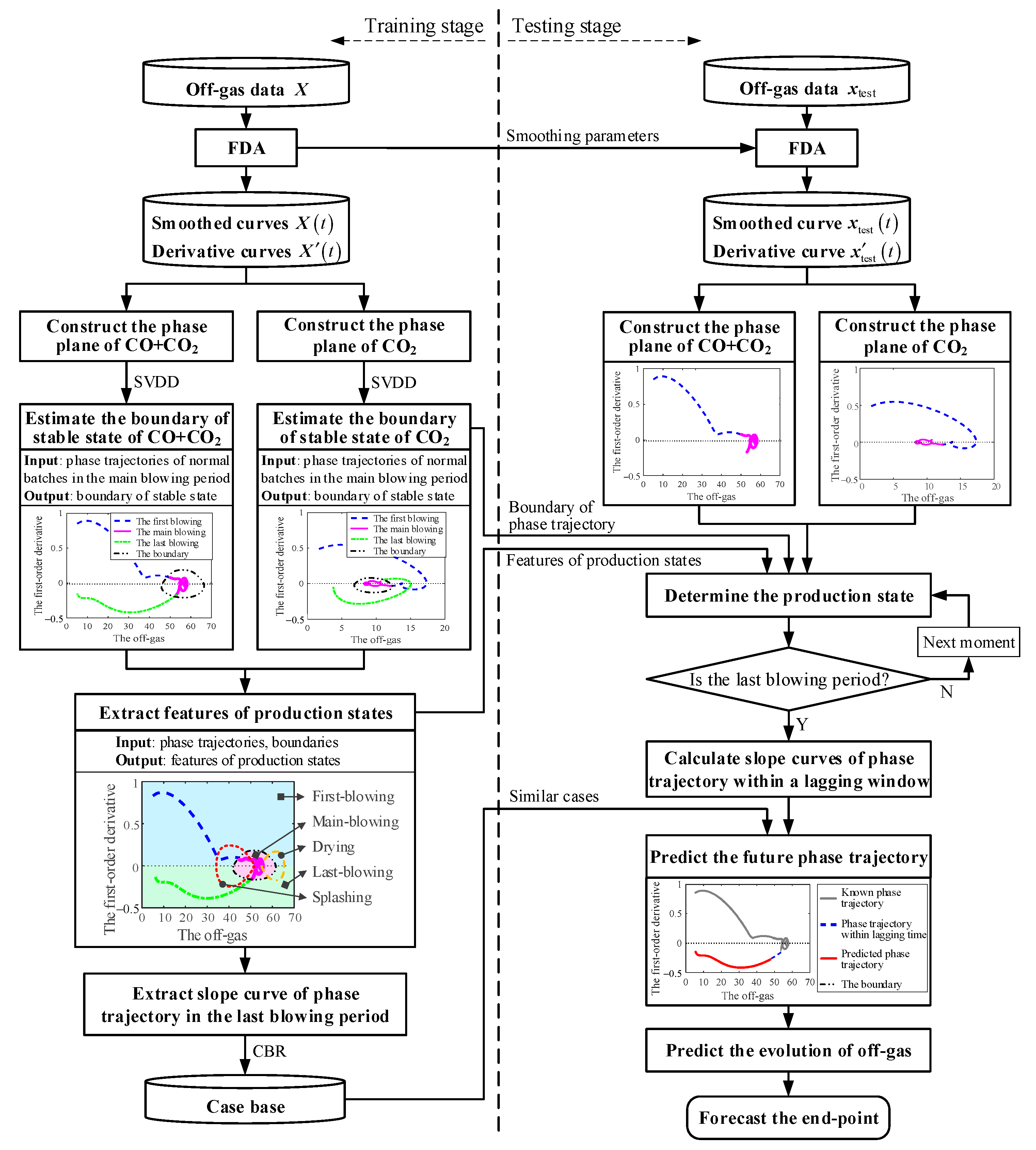
3.1. Extraction and Characterization of Dynamics Features

In order to describe and predict the production state of BOF steelmaking, the smoothed function and the first-order derivative function of off-gas compositions, i.e., the total proportion of CO and CO₂, are extracted by the FDA and then used to construct the phase plane to characterize the dynamics features of the decarburization reaction.

Functional data analysis [25] is a theory that regards a set of discrete observations as the sampling of a continuous function. Suppose $x\left(t\right)$ is a continuous function and $t={[\begin{array}{cccc}{t}_1& t_2& \dots & t_K\end{array}]}^{\mathrm{T}}$ is the sampling instant, then the discrete observations $\widehat{x}={[\begin{array}{cccc}{\widehat{x}}_1& {\widehat{x}}_2& \dots & {\widehat{x}}_K\end{array}]}^{\mathrm{T}}$ can be acquired as:

$$\widehat{x}=x\left(t\right)+e={\left[\begin{array}{cccc}x\left(t_1\right)& x\left(t_2\right)& \dots & x\left(t_K\right)\end{array}\right]}^{\mathrm{T}}+e$$

(1)

where $K$ is the number of sampling points and $e$ is the noise matrix. In order to express the continuous function $x\left(t\right)$, the FDA theory employs a linear combination of basis functions $\mathsf{\varphi }\left(t\right)={\left[\begin{array}{cccc}{\varphi }_1\left(t\right)& {\varphi }_2\left(t\right)& \dots & {\varphi }_N\left(t\right)\end{array}\right]}^{\mathrm{T}}$ to approximate the discrete observations $\widehat{x}$, which is as follows:

$$x\left(t\right)=\mathsf{\varphi }{\left(t\right)}^{\mathrm{T}}c=\widehat{x}-e$$

(2)

where $c={\left[\begin{array}{cccc}{c}_1& c_2& \dots & c_N\end{array}\right]}^{\mathrm{T}}$ is a coefficient vector associated with the basis function system $\mathsf{\varphi }\left(t\right)$. Usually, the coefficients $c$ are calculated by Least Squares with a roughness penalty item, i.e.,:

$$\underset{\mathit{e}}{\min } e^{\mathrm{T}}e=\underset{c}{\min }\left\{{\left(\widehat{x}-\mathsf{\varphi }{\left(t\right)}^{\mathrm{T}}c\right)}^{\mathrm{T}}\left(\widehat{x}-\mathsf{\varphi }{\left(t\right)}^{\mathrm{T}}c\right)+\lambda PE{N}_m\left[x\left(t\right)\right]\right\}$$

(3)

where $\mathsf{\varphi }\left(t\right)=\left[\begin{array}{cccc}{\varphi }_1\left(t_1\right)& {\varphi }_1\left(t_2\right)& \dots & {\varphi }_1\left(t_K\right)\\ {\varphi }_2\left(t_1\right)& {\varphi }_2\left(t_2\right)& \dots & {\varphi }_2\left(t_K\right)\\ \dots & \dots & \dots & \dots \\ {\varphi }_N\left(t_1\right)& {\varphi }_N\left(t_2\right)& \dots & {\varphi }_N\left(t_K\right)\end{array}\right]$ is the sampling matrix of the basis function vector $\mathsf{\varphi }\left(t\right)$, $PE{N}_m\left[x\left(t\right)\right]={\displaystyle \int {\left[D^{m}x\left(t\right)\right]}^{2}dt}$ is the roughness penalty that is an integrated squared linear differential operator to ensure the continuous control of the function’s smoothness, m is the derivative order of the roughness penalty, $\lambda$ is a parameter defining the smoothness of the fitted curve. According to Equation (3), the basis function coefficients are inferred to be:

$$c={\left[\mathsf{\varphi }\left(t\right)\mathsf{\varphi }{\left(t\right)}^{\mathrm{T}}+\lambda R\right]}^{-1}\mathsf{\varphi }\left(t\right)\widehat{x}$$

(4)

where $R={\displaystyle \int \frac{d^m\mathsf{\varphi }\left(t\right)}{d{t}^m}{\frac{d^m\mathsf{\varphi }\left(t\right)}{d{t}^m}}^{\mathrm{T}}dt}$. Substituting Equation (4) into Equation (2) will obtain the continuous function $x\left(t\right)$. The details to determine the tuning parameters, including the order of basis functions, the number of basis functions N, the derivative order of roughness penalty m, and the coefficient of roughness penalty $\lambda$, can be found in our previous work [16]. Then, with the continuous function obtained, we can extract their derivatives to reveal their underlying dynamical features. For example, the first-order derivative function can be calculated by the following equation to characterize the function’s instantaneous change rate over time.

$$x^{\prime }\left(t\right)=\frac{d\left[x\left(t\right)\right]}{dt}=\frac{d\left[\mathsf{\varphi }{\left(t\right)}^{\mathrm{T}}\right]}{dt}c$$

(5)

After the continuous function and the first-order derivative function of the total proportion of CO and CO₂ are obtained based on the theory of FDA, the phase plane can be constructed to characterize the dynamics features of BOF steelmaking. Here, the transverse axis is the total proportion of CO and CO₂, evaluating the reaction velocity of the decarburization reaction, and the longitudinal axis is the first-order derivative of the total proportion of CO and CO₂, evaluating the reaction acceleration of decarburization reaction. For other applications, other derivatives even some integration can be used to explain the system’s dynamics state.

After the phase plane is constructed, the evolution features of the phase trajectory are used to recognize different blowing periods and anomalies, as well as to predict end-point time.

3.2. Production State Recognition with Dynamics Features

According to the evolution features of phase trajectory described in Section 2.2, the boundary of the stable-state region is estimated via the SVDD [16] to determine the production state, where the phase trajectories of CO + CO₂ of normal batches in the main blowing period are used as the training dataset. The calculation of SVDD can be found in Appendix A. Since the phase trajectory of the splashing anomaly exceeds the stable-state region from the fourth quadrant as the phase trajectory of the last blowing period does, the phase plane of CO₂ is constructed to distinguish the splashing anomaly from the last blowing period. The boundary of the stable-state region of the CO₂ phase plane is also estimated via the SVDD.

Then, based on the phase trajectories and their boundaries, the production state is determined at each moment by successively checking whether the phase trajectory of CO + CO₂ exceeds the boundary of the stable-state region, whether the phase trajectory of CO + CO₂ exceeds the boundary from the left side, and whether the phase trajectory of CO₂ exceeds the boundary of the stable-state region. The check procedure is given in Figure 4. For example, if the previous production state is the main blowing period and the current phase trajectory of CO + CO₂ exceeds the boundary, the location of the phase trajectory of CO + CO₂ needs to be checked. If the phase trajectory of CO + CO₂ is on the left of the boundary, a further check of the phase trajectory of CO₂ is necessary to distinguish the splashing anomaly from the last blowing period; otherwise, we can infer that the drying anomaly happens.

3.3. End-Point Time Prediction with Dynamics Features

After the phase trajectory indicates that the last blowing period begins, the end-point time is forecast by predicting the phase trajectory in the last blowing period via case-based reasoning (CBR) [26]. The statement of CBR can be found in Appendix B. Here, the slope curves of the phase trajectories instead of the phase trajectories are employed as attributes to describe the cases/samples, since different batches have different ranges of phase trajectory in the last blowing period. And a lagging window is used to extract the former part of slope curves as the condition attributes and the latter part as the solution attributes. The similar cases are found out according to their distances to the testing case in the problem space are less than a threshold, and their solution attributes are averaged as the solution to the testing case.

The whole procedure of the proposed FDA-PP method is shown in Figure 5. This method firstly smooths the sampling sequences of off-gas data to continuous functions and extracts their first-order derivative functions to construct the phase plane to characterize the metallurgical dynamics features of BOF steelmaking. Then, based on the evolution features of phase trajectories, a boundary that indicates the region of stable production state is estimated to recognize different blowing periods as well as splashing and drying anomalies. Finally, when the last blowing period begins, the end-point time is forecast through referring to the completed batches with similar slope curves of phase trajectories.

4. Experiment on BOF Steelmaking

In this section, we validate the performance of the proposed FDA-PP method on the BOF steelmaking process.

4.1. Data Acquisition and Modeling Calculation

The data of BOF steelmaking are collected from a 260 tons converter in a Chinese steel plant. The proportions of CO and CO₂ in the off-gas are analyzed by the mass spectrometer with sampling frequency 0.5 Hz. Totally 476 batches/heats without re-blowing are selected, including 375 normal batches, 66 splashing batches, and 35 drying batches. The data partition can be found in

Table 1. Data partition of the steelmaking data.

	Normal	Abnormal		Total
		Splashing	Drying
Training	150	/	/	150
Testing	225	66	35	326
Total	375	66	35	476

. 150 normal batches are randomly selected for training and the rest 326 batches are used for testing.

In addition, the true end-point time is collected in Figure 6, which is calculated through subtracting the lagging time (30 s in this work) from the duration of the last blowing period. The true end-point time reflects how long in advance the FDA-PP method could predict the end-point. As seen in Figure 6, the true end-point time of over 90% batches is 100~240 s. Thus, the FDA-PP can be expected to predict the end-point and provide a time margin of about 2~4 min for operation optimization.

Following the calculation procedure in Figure 5, firstly, 30 B-splines basis functions with order 5 are used to smooth the off-gas compositions data and extract their first-order derivatives, where the roughness penalty is the integrated squared third derivative operator with $\lambda ={10}^5$. It should be noted that the time range of the fitting curve is equal to the actual blowing time of each batch. Based on the fitting curves and the first-order derivative curves, the phase plane of the total proportion of CO and CO₂ is built to characterize the production state, and the phase plane of CO₂ is built to help distinguish the splashing anomaly from the last blowing period. Then, the phase trajectories in the main blowing period are used to estimate the boundaries of the stable-state region for the production state recognition, where the bandwidths of RBF kernel are $\sigma =3$ for the phase plane of the total proportion of CO and CO₂ and $\sigma =1.5$ for the phase plane of CO₂. After that, the slope curves of phase trajectory in the last blowing period are recorded, where the slope curves within the lagging time window of 30 s (i.e., 15 sampling points) compose the condition attributes base and the slope curves after the lagging time window compose the solution attributes base. The criterion for similar case selection is that the Euclidean distance with the target batch ranks in the former 15%. Based on the predicted phase trajectory, the end-point time is finally estimated.

In order to further illustrate the performance of the proposed FDA-PP method, the classical phase space (PS) is calculated as comparisons, as well as two commonly used methods in BOF steelmaking, the SVM and the back-propagation neural network (BP). The details of these methods are summarized as follows:

• PS: This method sets the embedding dimension as 2 and the delay time as $\tau =5$ to construct the phase space, and uses the phase trajectories to complete the rest calculation procedures as the FDA-PP method does.
• SVM: This method is calculated with 13 process variables, including the information of raw materials (i.e., the temperature of molten iron, the carbon content, silicon content, manganese content, phosphorus content of molten iron, the weight of molten iron, the weight of pig iron, the weight of scrap steel), the cumulative weight of auxiliary materials, and the operation parameters (i.e., the total proportion of CO and CO₂, the height of oxygen lance, the cumulative volume of oxygen blowing, the flow of bottom blowing). Among them, the information of auxiliary materials and operation parameters is recorded as sequences. Since the SVM is a supervised classification method, 10 normal batches, 10 splashing batches, and 10 drying batches are trained for production state recognition. For the end-point time prediction, still 150 normal batches are used for training.
• BP: This method is carried out with the same variables and data partition as the SVM method does, where the size of the hidden layer is set as 60 for the production state recognition and 5 for the end-point prediction.

To avoid randomness of individual results, the FDA-PP method as well as all the compared methods are tested 50 times based on the random data partition. The results are discussed in the following sections.

4.2. Results of the Production State Recognition

Table 2. Accuracy of production state recognition.

Method	Blowing Periods Recognition of Normal Batches			Anomaly Identification of Abnormal Batches
	First-Blowing	Main-Blowing	Last-Blowing	Splashing Anomaly	Drying Anomaly
FDA-PP	99.16%	87.78%	88.49%	90.94%	81.29%
PS	98.22%	82.33%	84.13%	67.00%	74.29%
SVM	87.28%	66.67%	71.93%	62.12%	54.55%
BP	65.59%	43.21%	50.26%	30.30%	41.67%

shows the accuracy of the production state recognition. For the normal batches, we collect the recognition accuracies of the first blowing period, the main blowing period, and the last blowing period, where correctly identifying the blowing periods not only provides guidance for process control but also gives a start signal for the end-point time prediction. For the abnormal batches, we collect the recognition accuracies of the splashing and drying anomalies, where correctly alarming the anomalies can help workers take action to restrain the anomalies.

Table 2 illustrates that the proposed FDA-PP method has the best accuracy on the production state recognition, where the blowing period recognition accuracy of normal batches is 87.78%, the anomaly identification accuracies of splashing and drying batches are 90.94% and 81.29% respectively. For the compared methods, the PS method has lower accuracy than the FDA-PP method because the difference calculation in the PS method would bring errors in expressing the off-gas composition’s variation and cannot isolate the noise interference. The SVM and BP methods are inferior to the FDA-PP method and the PS method although they utilize 13 variables to take the information of raw materials, auxiliary materials, and operation parameters into consideration. This result demonstrates that the dynamics features expressed by the phase plane and phase space are significant in determining a system’s operating condition. For BOF steelmaking, different blowing periods and anomalies would generate similar production data. The SVM and BP methods analyze the measurements at an individual moment and miss the evolution features of the sequence within an interval, so easily confuses different production states. The FDA-PP and PS methods not only indicate the decarburization rate but also describe how the decarburization rate is going to change with the influence of operation parameters, so have better performance on the production state recognition.

We take a splashing batch and a drying batch as examples to show the results of production state recognition, as can be seen in Figure 7. The FDA-PP method successfully recognizes the three blowing periods as well as the splashing and drying anomalies. The PS method successfully identifies the drying batch but confuses the splashing anomaly with the last blowing period. The SVM method identifies different blowing periods but misses catching the drying anomaly, and it gives a false alarm before the splashing anomaly. The BP method nearly cannot judge the production state of the splashing batch and falsely regards the drying as the splashing.

Furthermore, as the production state is recognized at each sampling point, the FDA-PP method is able to be implemented on the online characterization, where the production state at sampling point t is recognized using the sequence from the start point to the current point.

4.3. Results of the End-Point Time Prediction

Based on the production state recognition, the end-point time is going to be predicted as the last blowing period begins. Thus, the ending time prediction is a forecast ahead of time and can be available for the online application, where the end-point can be predicted using the sequence within the lagging time during the last period.

Table 3. MRPE of end-point time prediction.

Method	Normal Batches	Splashing Batches	Drying Batches	Mean Value
FDA-PP	18.07%	19.31%	17.01%	18.13%
PS	41.36%	49.79%	46.91%	46.02%
SVM	19.53%	31.28%	26.78%	25.86%
BP	19.44%	32.58%	29.94%	27.32%

collects the mean relative prediction error (MRPE) of the end-point time, which is calculated as follows:

$$\delta =\frac{1}{N}·\frac{\left|\Delta {\widehat{t}}_n-\Delta t_n\right|}{\Delta t_n}$$

(6)

where $\Delta t_n$ is the true value of the end-point time of batch n which is calculated through subtracting the lagging time (30 s in this work) from the duration of the last blowing period, $\Delta {\widehat{t}}_n$ is the predicted value of the end-point time of batch n, and N is the number of batches. For the SVM and BP methods, since Section 4.2 indicates that they can hardly identify different blowing periods, the beginning moment of the last blowing period in the SVM and BP methods is provided by the FDA-PP method.

From Table 3 we can see that the proposed FDA-PP method is much more accurate than the PS method and more accurate on the abnormal batches than the SVM and BP methods. The FDA-PP method can predict the ending time with MRPE 18.07%. Especially when the splashing or drying anomaly happens, the MRPE of the end-point time can be controlled within 20%. As for the SVM and BP methods, although they achieve similar MRPE on the normal batches as the FDA-PP method, their prediction errors on the abnormal batches are about 10% larger than the FDA-PP method. The superiority of FDA-PP on the abnormal batches is due to that the FDA-PP method predicts the end-point through estimating the evolution of dynamics features (the phase trajectory) but the SVM and BP methods only utilize the measurements of production data. When the anomalies happen, the dynamics features would change, and the decarburization reaction rate would be influenced, bringing difficulties in end-point prediction. Therefore, the SVM and BP methods have larger prediction errors on the abnormal batches.

Figure 8 shows the distribution of the absolute deviation of the predicted end-point time, i.e., the numerator in Equation (6). As can be seen in Figure 8, using the FDA-PP method, the end-point time prediction of more batches can be controlled in smaller absolute deviations than the PS, SVM, and BP methods, especially of the abnormal batches. The FDA-PP method can ensure the absolute deviation of the predicted end-point time on 20% splashing batches and 27% drying batches no more than 10 s, and on 60% splashing batches and 61% drying batches no more than 30 s. As comparison, the PS, SVM, and BP methods can hardly control the absolute deviation on abnormal batches to be in 10 s, and their ratios of abnormal batches whose absolute deviations are no more than 30 s are less than the FDA-PP method.

More physical insights into the production state prediction of BOF steelmaking are that, first, with the predicted phase trajectory, the evolution of the total proportion of CO and CO₂ in the last blowing period can be reconstructed, then further studies such as the steel compositions prediction and the temperature prediction can be realized associated with information of raw materials and operation parameters. Second, although the FDA-PP method only utilizes the off-gas data, it realizes similar even better performance than the SVM and BP methods that process variables; thus, the off-gas can be expected to replace the sub-lance to control the BOF steelmaking so that avoiding the production process suspension.

5. Conclusions

This work aims at the production state recognition and the end-point time prediction, and proposes a new data-based method associated with the off-gas data, defined as FDA-PP. This method describes the evolution of the production state from the metallurgical dynamics viewpoint and takes a comprehensive consideration of the decarburization rate as well as its variation trend. As the change of off-gas compositions was only used to recognize the splashing and drying anomalies in the existing research, this work is an attempt that using the off-gas data to distinguish different blowing periods and predict the end-point time.

In order to evaluate the performance of the proposed method, the real production data from a steel plant are studied. The results show that the FDA-PP method achieves the production state recognition accuracy at 87.78% for normal batches, 90.94% for splashing batches, and 81.29% for drying batches, respectively, more accurate than the PS, SVM, and BP methods. At the same time, the MRPE of end-point time prediction by the FDA-PP method is lower than the compared methods. Especially on the abnormal batches, although the FDA-PP method only employs the proportions of CO and CO₂ in the off-gas, its prediction error of ending time is about 10% lower than the SVM and BP methods that utilize 13 variables to take the information of raw materials, auxiliary materials, and operation parameters into consideration. Moreover, the FDA-PP method can predict the end-point time once the model judges that the last blowing period begins, so providing 2~4 min time margin for the operation parameters optimization.

Following this work, the predicted sequences of the total proportion of CO and CO₂ by the FDA-PP method give a possibility to predict the steel compositions and temperature. In addition, more efforts can be devoted to exploring the use of off-gas information for production control so that replacing the sub-lance and ensuring continuous production rhythm.

References

1. World Steel Association. Fact Sheet: Steel and Raw Materials. Available online: https://worldsteel.org/steel-topics/statistics/world-steel-in-figures-2022/#crude-steel-production-by-process-2021 (accessed on 3 November 2022).
2. De Vos, L.; Bellemans, I.; Vercruyssen, C.; Verbeken, K. Basic Oxygen Furnace: Assessment of Recent Physicochemical Models. Metall. Mater. Trans. B 2019, 50, 2647–2666. [Google Scholar] [CrossRef]
3. Heenatimulla, J.; Brooks, G.A.; Dunn, M.; Sly, D.; Snashall, R.; Leung, W. Acoustic Analysis of Slag Foaming in the BOF. Metals 2022, 12, 1142. [Google Scholar] [CrossRef]
4. Singha, P.; Shukla, A.K. Contribution of Hot-Spot Zone in Decarburization of BOF Steel-Making: Fundamental Analysis Based upon the FactSage-Macro Program. Metals 2022, 12, 638. [Google Scholar] [CrossRef]
5. Shanmugam, S.P.; Nurni, V.N.; Manjini, S.; Chandra, S.; Holappa, L.E.K. Challenges and Outlines of Steelmaking toward the Year 2030 and Beyond—Indian Perspective. Metals 2021, 11, 1654. [Google Scholar] [CrossRef]
6. Zhou, D.; Xu, K.; Lv, Z.; Yang, J.; Li, M.; He, F.; Xu, G. Intelligent Manufacturing Technology in the Steel Industry of China: A Review. Sensors 2022, 22, 8194. [Google Scholar] [CrossRef] [PubMed]
7. Nenchev, B.; Panwisawas, C.; Yang, X.; Fu, J.; Dong, Z.; Tao, Q.; Gebelin, J.-C.; Dunsmore, A.; Dong, H.; Li, M.; et al. Metallurgical Data Science for Steel Industry: A Case Study on Basic Oxygen Furnace. Steel Res. Int. 2022, 93, 2100813. [Google Scholar] [CrossRef]
8. Wang, R.; Mohanty, I.; Srivastava, A.; Roy, T.K.; Gupta, P.; Chattopadhyay, K. Hybrid Method for Endpoint Prediction in a Basic Oxygen Furnace. Metals 2022, 12, 801. [Google Scholar] [CrossRef]
9. Zou, Y.; Yang, L.; Li, B.; Yan, Z.; Li, Z.; Wang, S.; Guo, Y. Prediction Model of End-Point Phosphorus Content in EAF Steelmaking Based on BP Neural Network with Periodical Data Optimization. Metals 2022, 12, 1519. [Google Scholar] [CrossRef]
10. Han, M.; Zhao, Y. Dynamic control model of BOF steelmaking process based on ANFIS and robust relevance vector machine. Expert Syst. Appl. 2011, 38, 14786–14798. [Google Scholar] [CrossRef]
11. Fei, H.; Xianyi, C.; Zhenghai, Z. Prediction of oxygen-blowing volume in BOF steelmaking process based on BP neural network and incremental learning. High Temp. Mater. Process. 2022, 41, 403–416. [Google Scholar] [CrossRef]
12. Zhao, D. Research on Prediction of Converter Endpoint Based on Image Processing. Master’s Thesis, Inner Mongolia University of Science and Technology, Baotou, China, 2020. [Google Scholar]
13. Li, A.; Li, C.; Wang, Y.; Cui, G.; Xie, S. Recognition of converter blowing periods based on improved DenseNet Network. J. Univ. Jinan 2022, 36, 273–277. [Google Scholar] [CrossRef]
14. Wen, H. Research on Modeling and Prediction of BOF End-Point Based on the Furnace Mouth Radiation Information. Ph.D. Thesis, Nanjing University of Science and Technology, Nanjing, China, 2009. [Google Scholar]
15. Brämming, M.; Bjorkman, B.; Samuelsson, C. BOF process control and slopping prediction based on multivariate data analysis. Steel Res. Int. 2016, 87, 301–310. [Google Scholar] [CrossRef]
16. Qian, Q.; Fang, X.; Xu, J.; Li, M. Multichannel profile-based anomaly detection and its application in the monitoring of basic oxygen furnace steelmaking process. J. Manuf. Syst. 2021, 61, 375–390. [Google Scholar] [CrossRef]
17. Li, G.-H.; Wang, B.; Liu, Q.; Tian, X.-Z.; Zhu, R.; Hu, L.-N.; Cheng, G.-G. A process model for BOF process based on bath mixing degree. Int. J. Miner. Metall. Mater. 2010, 17, 715–722. [Google Scholar] [CrossRef]
18. Wang, Z. Study on the Control of Steelmaking Process and Blowing End-Point for Medium-High Carbon Steel Melting by Converter. Ph.D. Thesis, University of Science and Technology Beijing, Beijing, China, 2016. [Google Scholar]
19. Li, N.; Lin, W.; Cao, L.; Liu, Q.; Sun, L.; Liao, S. Carbon prediction model for basic oxygen furnace off-gas analysis based on bath mixing degree. Chin. J. Eng. 2018, 40, 1244–1250. [Google Scholar] [CrossRef]
20. Rahnama, A.; Li, Z.; Sridhar, S. Machine Learning-Based Prediction of a BOS Reactor Performance from Operating Parameters. Processes 2020, 8, 371. [Google Scholar] [CrossRef] [Green Version]
21. Dering, D.; Swartz, C.L.; Dogan, N. A dynamic optimization framework for basic oxygen furnace operation. Chem. Eng. Sci. 2021, 241, 116653. [Google Scholar] [CrossRef]
22. Deo, B.; Overbosch, A.; Snoeijer, B.; Das, D.; Srinivas, K. Control of Slag Formation, Foaming, Slopping, and Chaos in BOF. Trans. Indian Inst. Met. 2013, 66, 543–554. [Google Scholar] [CrossRef]
23. Bae, S.; Mo, D.Y. Dynamical analysis of an anemoscope in the phase plane. Appl. Math. Model. 2010, 34, 1884–1891. [Google Scholar] [CrossRef]
24. Han, Z.; Xu, N.; Chen, H.; Huang, Y.; Zhao, B. Energy-efficient control of electric vehicles based on linear quadratic regulator and phase plane analysis. Appl. Energy 2018, 213, 639–657. [Google Scholar] [CrossRef]
25. Ramsay, J.O.; Silverman, B.W. Functional Data Analysis, 2nd ed.; Springer: New York, NY, USA, 2005. [Google Scholar]
26. Han, M.; Li, Y.; Cao, Z. Hybrid intelligent control of BOF oxygen volume and coolant addition. Neurocomputing 2014, 123, 415–423. [Google Scholar] [CrossRef]
Figure 1. The schematic representation of BOF steelmaking.
Metals 13 00002 g001
Figure 2. (a) The schematic representation of different blowing periods; (b) the off-gas compositions of a normal batch; (c) the off-gas compositions of a splashing batch; (d) the off-gas compositions of a drying batch.
Metals 13 00002 g002
Figure 3. The phase plane of (a) normal batch; (b) splashing batch; (c) drying batch.
Metals 13 00002 g003
Figure 4. The check procedure for production state characterization.
Metals 13 00002 g004
Figure 5. The schematic diagram of the proposed FDA-PP method.
Metals 13 00002 g005
Figure 6. Distribution of the true end-point time.
Metals 13 00002 g006
Figure 7. (ad) Production state recognition of a splashing batch by different methods; (eh) production state recognition of a drying batch by different methods. Here, the events indicate that: 1-the first blowing period, 2-the main blowing period, 3-the main blowing period, 4-the splashing anomaly, 5-the drying anomaly.
Metals 13 00002 g007
Figure 8. Absolute deviation of the predicted end-point time on (a) the normal batches, (b) the splashing batches, (c) the drying batches.
Metals 13 00002 g008