Article

Effect of Local Fluid Disturbance Induced by Weld Reinforcement Height on the Corrosion of a Low Alloy Steel Weld

1
CAS Key Laboratory of Nuclear Materials and Safety Assessment, Institute of Metal Research, Chinese Academy of Sciences, 62 Wencui Road, Shenyang 110016, China
2
School of Materials Science and Engineering, University of Science and Technology of China, Shenyang 110016, China
3
China Nuclear Power Operation Management Co., Ltd., Haiyan 314300, China
*
Authors to whom correspondence should be addressed.
Metals 2023, 13(1), 103; https://doi.org/10.3390/met13010103
Submission received: 8 November 2022 / Revised: 25 December 2022 / Accepted: 30 December 2022 / Published: 3 January 2023

Abstract

:
Weld corrosion exists widely in the petrochemical industry and attracts great attention. Most research proves that weld corrosion originates from the material factors introduced during the welding process. However, it is noted that local fluid turbulence due to the weld reinforcement height (WRH) plays an important role in the non-uniform corrosion of welds in flowing media. Accordingly, the individual effect of the local flow on the weld corrosion of low alloy steel was analyzed by experiments and simulation in this study. Electrochemical measurements and morphology observation were conducted, combined with flow field analyses. The results showed that local fluid turbulence due to WRH affected the non-uniform corrosion of low alloy steel welds. The upstream surface and the backflow surface had the highest and lowest corrosion rates, respectively. Interestingly, the high flow velocity surface region did not have a high-corrosion rate. This is due to the combined effects of mass transfer, charge transfer, and wall shear stress. The pitting corrosion was also discussed in view of the aspects above.

1. Introduction

Weld corrosion is a common form of corrosion in the oil and gas industry [1,2,3,4]. It is undeniable that most of them are related to the changes in material factors resulting from the thermal effects of the welding process, such as microstructure and element distribution [5,6,7,8]. However, localized corrosion is prone to occur in regions where the flow status changes suddenly, such as in rapid expansion pipes [9,10], gradual contraction pipes [11], pitting defects [12,13], and the orifice [14,15]. It has been proved that the local fluid turbulence due to the sudden change of geometry has significant effects on corrosion [11,12,14]. Therefore, the sudden change of the local flow conditions caused by the weld bulge cannot be ignored for the welds serving in flowing media.
Weld reinforcement height (WRH) protrudes from the flow surface and introduces local fluid disturbance to the flow field [16,17]. This local fluid turbulence affects the corrosion in two ways. One is the mass transfer [17,18,19,20], and the other one is the wall shear stress (WSS). For the former, the non-streamline profile of the weld can destroy the original fluid boundary layer [21,22] and diffusion layer resulting in different driving forces of the mass transfer [23,24]. It is generally considered that the higher the flow velocity, the faster the mass transfer rate and the higher the corrosion rate [11]. There is also an argument that the flow velocity does not have a monotonic relationship with corrosion [25,26]. Tomarov et al. [23] found that local erosion-corrosion was the dominant mechanism causing thinning of the welded connections in the pipelines of a power unit at a nuclear power station. Hosseini et al. [24] investigated the effect of excessive penetration of welding on the sand erosion of elbows and reducers. They showed that the erosion rate increased by increasing excessive penetration. Most of the investigations focus on the corrosion of the entire weld. Moreover, the fluid turbulence effects on the corrosion of the elbows [27], expands [9], and orifices [14,15] have been reported. In contrast, little attention is paid to the relationship between localized weld corrosion and the surrounding fluid status.
In addition to the mass transfer, WSS is the other way that fluid turbulence influences corrosion [28,29]. It forms and acts on the material surface due to the fluid viscosity [12]. It is generally accepted that WSS can destroy the corrosion product film under flow conditions [1,19]. In contrast, some controversy proposed that the WSS was not high enough to remove the corrosion product film from the matrix [30]. For the WSS around WRH, it is enhanced due to the local flow turbulence. However, no related investigation can be referred to if the enhanced WSS can affect the corrosion up to now. The role played by WSS in the corrosion of the weld and its upstream and downstream areas is still unclear.
In this work, the corrosion behavior at different positions of the weld is studied. A new rotating disk with WRH was designed and used to examine the local turbulence effect on corrosion around the WRH combined with computational fluid dynamics (CFD). Different from the method employed in published works (elbow [3,19], rapidly expanding pipe [10], gradual contraction pipe [11]), this test rig concentrated on the corrosion differences on the weld instead of the special pipes. The corrosion behavior on different surfaces of the WRH was investigated by a homemade rotating disk electrode (RDE) with a weld-like bump. An optical microscope (OM), scanning electron microscope (SEM), energy dispersive spectrometer (EDS), and white light interferometer were used to observe the corrosion morphology of the samples. The effects of the mass transfer and the WSS were also discussed. The objective of this work is to clarify the correlation between the geometry of the weld area and the corrosion rate under flow conditions.

2. Experimental

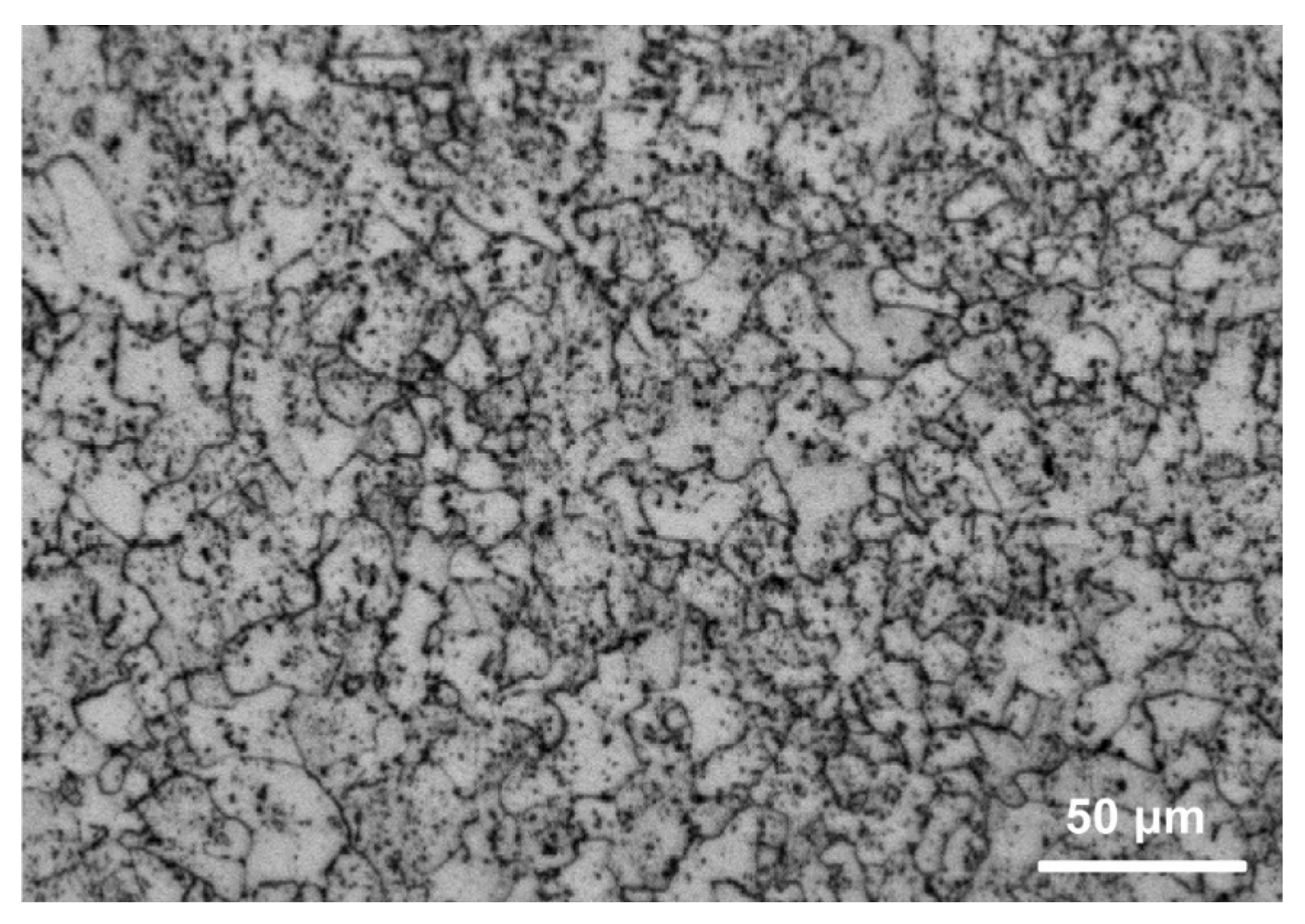
2.1. Materials and Specimens

The sample material was 1Cr5Mo low alloy steel, with a composition (wt. %) of 0.13 C, 0.34 Si, 0.47 Mn, 0.009 P, 0.0022 S, 4.68 Cr, 0.056 Ni, 0.5 Mo, 0.061 Cu, and Fe balance. The microstructure was observed using the sample that was polished by abrasive paste (2#) and subsequently etched in the 4% Nital solution for 5~10 s, according to ASTM E407-07(2015). Figure 1 displays the original microstructure of the studied 1Cr5Mo low alloy steel, showing metallographic structures of pearlite and ferrite grains with carbide precipitates [31]. The samples used for electrochemical tests were encapsulated in epoxy resin with an exposed area of 0.07 cm2. Before the experiments, the sample surface was mechanically ground using a series of silicon carbide paper up to 800 grit, then rinsed with deionized water and ethanol, and finally dried in hot air.

2.2. RDE Apparatus and Testing Conditions

An RDE test system was employed to perform the main flow corrosion tests, whose schematic diagram is shown in Figure 2 [32,33]. The rotating disk in the RDE test system was newly designed for the geometry simulation of the WRH. Dimensions of the WRH were determined as a width of 16 mm and height of 5 mm according to EN ISO 5817 (2014) [34]. The distribution of samples and the trapezoidal bump is shown in Figure 3. Three trapezoidal pumps were performed on the disk at 120° to simulate the WRH (Figure 3a). Five positions were placed for the samples to detect the local corrosion and flow information, including the upstream surface (u1), incident flow surface (i2), the top surface (t3), backflow surface (b4), and downstream surface (d5). The samples were positioned in the middle of the radius of the rotating disk to avoid the influence of turbulence on the sample surface caused by the edge of the disk (Figure 3b). Each sample surface was kept in a plane where the sample was.
The composition of the test medium was 8870 mg/L Na+ and K+, 370 mg/L Ca2+, 82 mg/L Mg2+, 13120 mg/L Cl, 24 mg/L SO42−, and 550 mg/L HCO3. The solution with a pH of 7.11 simulated the injected water in some oilfields. The test solution consisted of analytic-grade reagent and ultra-pure deionized water with a resistivity of 18.25 MΩ cm. The experiment was conducted at room temperature, and the linear flow velocity of the sample center was 2.3 m/s.

2.3. Electrochemical Measurements

A Gamry Interface 1000 electrochemical test system with a three-electrode cell was used for electrochemical measurements. The electrochemical samples were used as the working electrode (WE), a graphite rod as the counter electrode (CE), and a saturated calomel electrode (SCE) with a salt bridge as the reference electrode (RE). The potentials were standard potentials relative to SCE. Electrochemical impedance spectroscopy (EIS) and linear polarization resistance (LPR) curves were measured after the stabilization of open circuit potential (OCP). EIS measurements were performed at OCP with a sinusoidal alternating amplitude of 10 mV and a frequency from 10,000 Hz ~ 0.1 Hz [35,36]. LPR test was performed at −10 mv vs.OCP ~ +10 mv vs.OCP and a scanning rate of 0.125 mv/s. The electrochemical test started after 1 h flow corrosion. The data post-processing was performed using Gamry Echem Analyst 6.33 software (Gamry Instruments, Inc., Warminster, PA, USA).

2.4. Characterization of Corrosion Products and Corrosion Morphologies
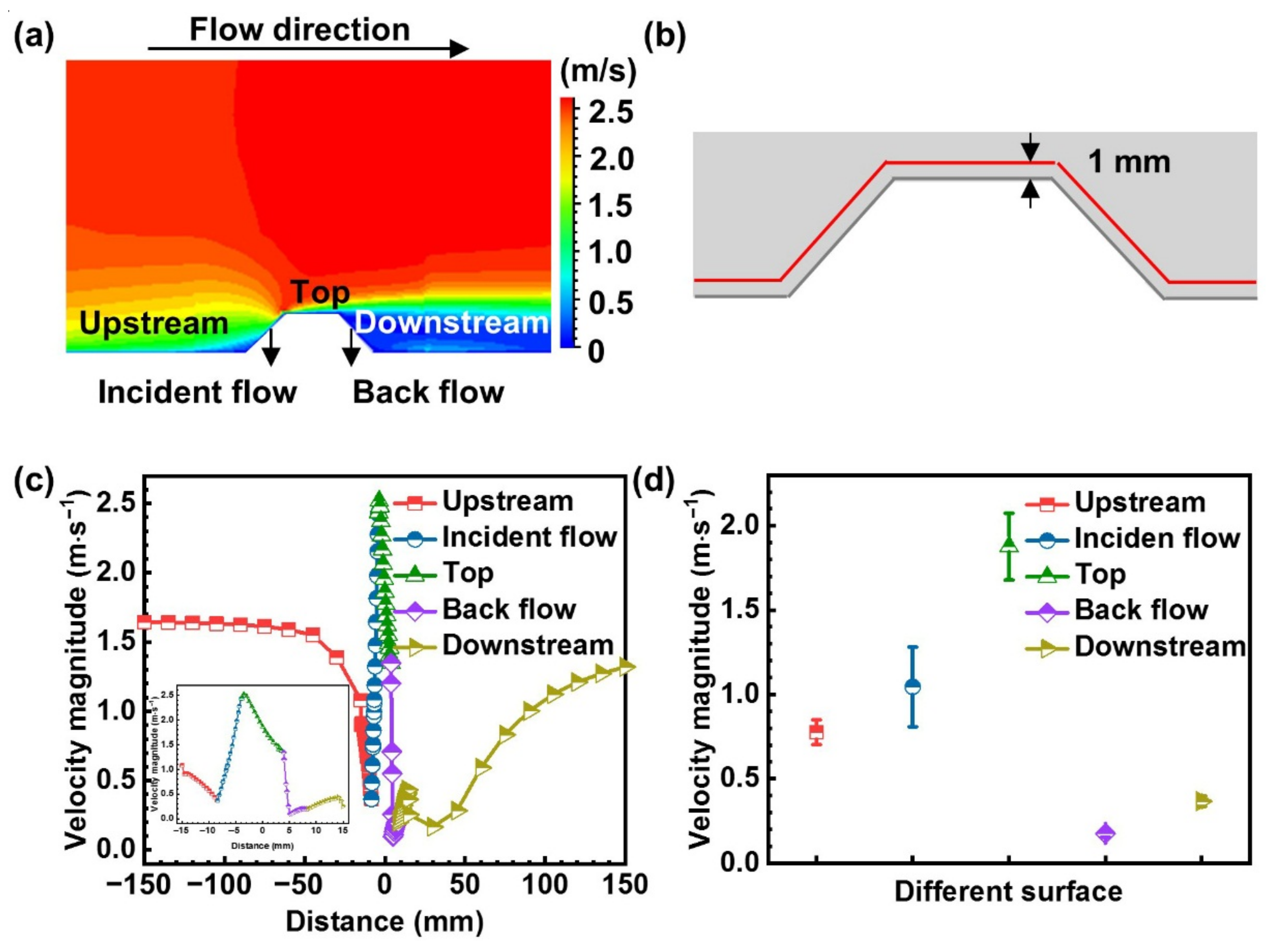
The samples were immersed in deionized water for 30 s after the experiment to remove the residual chemicals on the surface and avoid crystallization, then acid pickling was utilized to remove the corrosion products using the solution of 500 mL hydrochloric acid, 3.5 g hexamethylenetetramine, and deionized water, with a total volume of 1000 mL, according to ASTM G1-03 (2017) standard [37]. OM (Carl Zeiss Axio Observer. Z1m, Germany), SEM (Quattro S, FEI, USA), and white light interferometer (MicroXAM-3D, KLA, USA) analyses were performed on the sample surface before and after the removal of corrosion products to evaluate the damage caused by flow corrosion.

2.5. CFD Simulation

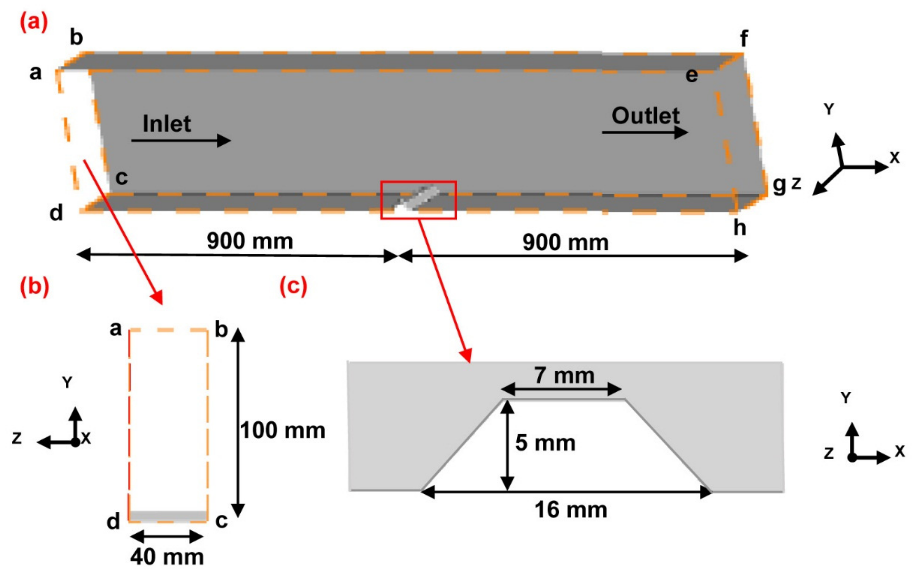
2.5.1. Geometric Model

CFD was used to capture the local flow information around the WRH. Figure 4 shows the geometric model of the WRH established by Gambit 2.4.6 software (ANSYS, Inc., Arbor, MI, USA). Its entrance and exit are rectangles of 40 × 100 mm, and the plane “adhe” is a symmetry plane. Both the inlet and outlet lengths are 10 times the hydraulic diameter to ensure that the flow is fully developed in the calculation process to avoid the inlet and outlet effects. Similar CFD works simulating fluids flowing over uneven surfaces could also be seen in the literature [32,33].

2.5.2. Fluid Flow Model

Commercial code, ANSYS Fluent 14.5 (ANSYS, Inc., Arbor, MI, USA), was used to simulate fluid flow in the pipe. The continuous flow is described by the continuity equation below.
t ( α i ρ i ) + ( α i ρ i v i ) = 0
where α i , ρ i and v i are the volume fraction, density, and velocity of the i phase, respectively.
The momentum equation is calculated below
( α i ρ i v i 2 ) = α i P + [ α i ( μ l , i + μ t , i ) v i + S i U ]
where μ l , i and μ t , i are the molecular viscosity and turbulent viscosity for the i phase, respectively, S i U = ρ i α i g + F i is the momentum source terms for the i phase, g is the gravitational acceleration vector, and F i is the interphase drag force for the i phase, respectively.
The k-epsilon turbulence model, a typical two-function model, was used for the flow with a high Reynolds number. The interaction was solved by the standard wall function. The SIMPLEC algorithm was employed to solve pressure-velocity coupling functions [17], which is good for the convergence and stability of the calculation [38].

2.5.3. Boundary Conditions

For the fluid flow model, the inlet flow velocity was set as 2.3 m/s to simulate the flow test conditions of the rotating disk. It is the same as that used in the experiments. The atmospheric pressure was set to the outlet pressure. The internal flow medium is liquid water, with a density of 998.2 kg/m3 and a viscosity of 0.001003 kg/m·s. The effect of gravity was considered in the simulation with the value of 9.8 m/s2 in the negative direction of the Y-axis. Turbulent intensity I = 0.16 ( u l v ) 1 / 8 . When the rectangular cross-section is filled with fluid, the hydraulic diameter D H = 4 H W 2 H + W = 2 H W H + W , therefore, the turbulent boundary conditions at the entrance in this simulation are 3.47% turbulent intensity and 88.9 mm hydraulic diameter, respectively.

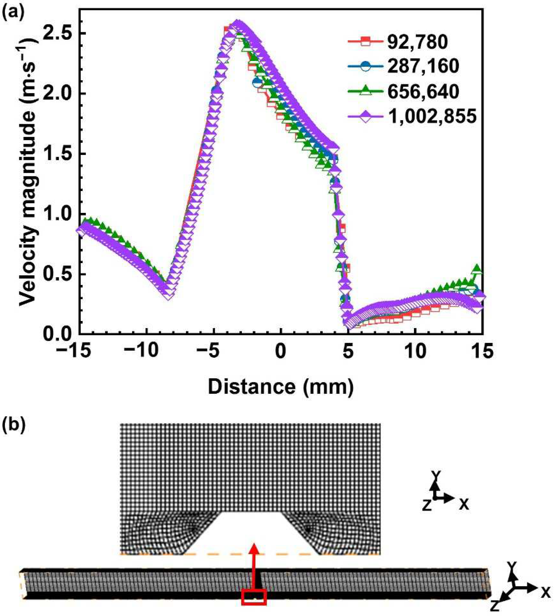
2.5.4. CFD Model Mesh

Before the formal simulation, grid-independent work was carried out. A curve was defined in the symmetry plane “adhe”, which was 1 mm away from each WRH plane. The flow velocity on this curve was read and compared at different grid conditions. The flow velocity distribution on the monitoring line is present in Figure 5a. Four groups of grids were selected to study the grid effect on the flow parameters. The grid numbers of hexahedral cells from coarse to fine were 92,780, 287,160, 656,640, and 1,002,855, respectively. It can be observed that the flow velocity varies little when the mesh number increases to 656,640 hexahedral cells. Therefore, this grid code with 683,478 nodes was used in the main simulation. Figure 5b shows the hexahedral mesh of the fluid domain and the local magnification of the WRH region. The meshes near the WRH wall are specially refined, which captures the flow parameters near the surface more accurately.

3. Results

3.1. Electrochemical Measurements Analysis
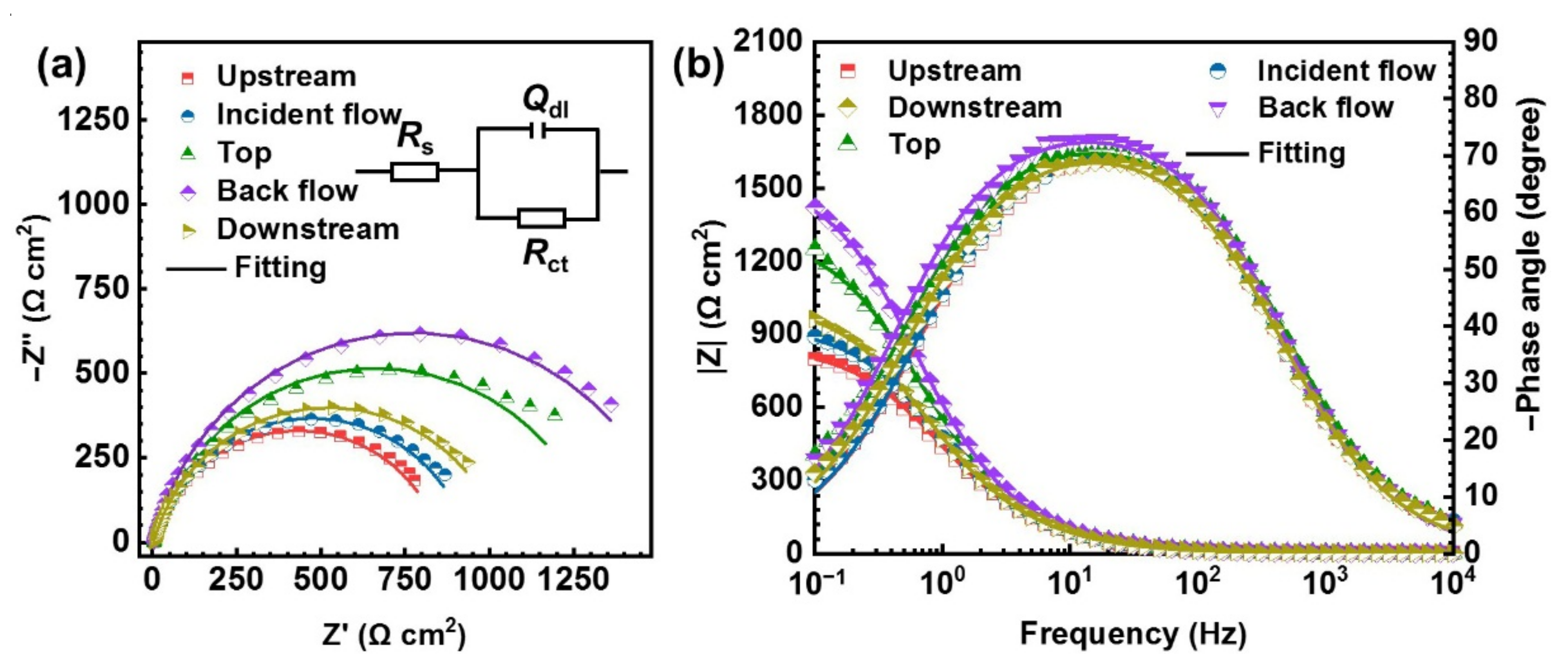
3.1.1. EIS Analysis

Figure 6 shows the Nyquist and Bode plots of the samples on different planes of WRH. All the Nyquist plots are characterized by capacitive semicircles in the high-frequency range (Figure 6a). Capacitive semicircle is related to interfacial charge transfer reaction [39,40,41]. The diameter of the high-frequency capacitive semicircle in Nyquist plots increases gradually in the following order: upstream surface < incident flow surface < downstream surface < top surface < backflow surface. The impedance values at 0.1 Hz in the Bode plots follow the same trend. High impedance indicates high corrosion resistance [42]. Therefore, the corresponding corrosion rate relationship is upstream surface > incident flow surface > downstream surface > top surface > backflow surface.
To obtain the EIS parameters, an equivalent circuit with one time constant (Figure 6a) was used to fit the EIS curves, where Rs is solution resistance, Rct is charge transfer resistance related to the process at the steel/solution interfaces, and Qdl is double layer capacitance. Table 1 lists the fitted EIS parameters. The larger the Rct value is, the lower the corrosion rate is [43]. The Rct value on the backflow surface is about twice that on the upstream surface. It indicates that the upstream sample suffers higher corrosion as compared to the sample on the backflow surface. Such a difference in corrosion could be caused by the flow conditions on the surface of each sample since the two samples are made of the same materials and immersed in the same solution.

3.1.2. LPR Analysis

The Rp values of each specimen were obtained by measuring the LPR, and the results are shown in Figure 7. Corrosion rates are directly proportional to 1/Rp [10]. The Rp increases along the flow direction to the maximum value on the backflow surface and then reduces on the downstream surface. The maximum Rp is on the backflow surface, which is about 1.5 times that on the upstream surface. Obvious Rp differences can be distinguished from different surfaces. It suggests that the local fluid turbulence due to WRH has a significant effect on local corrosion.

3.2. Surface Characterization Analysis

3.2.1. Corrosion Morphologies before Removing Corrosion Products

SEM corrosion morphologies of the samples located on different surfaces of the WRH with corrosion products are shown in Figure 8. Some corrosion products may be removed by fluid flow, which can be proved by the trace after the spalling of the corrosion products as circled (Figure 8a). The morphologies featured by comet tails can be identified for all cases, which are related to the corrosion products and were also observed in other studies [44,45]. By comparing the morphologies of samples on different surfaces, it can be found that the comet tails are different in number and size. The corrosion products on the top (Figure 8c) and backflow (Figure 8d) surfaces are less, while they are densely distributed and abundant on upstream, incident flow, and downstream surfaces. The larger area covered by corrosion products indicates severer corrosion. Meanwhile, the comet tails become shorter as the flow velocity increases [45]. Therefore, compared with the upstream, incident flow, and top surfaces, the longer comet tail on the backflow and downstream surfaces may be related to the lower flow velocity.
Figure 9 shows the SEM morphologies and elemental X-ray mapping of the five surfaces around the WRH after corrosion for 6 h in the flow direction. The contents of the main elements of the corrosion products are listed in Table 2. Convex corrosion products with tails cover the steel surface locally for all surfaces, and all the convex corrosion products of the samples on different surfaces have cracks indicating their loose structures. Moreover, the corrosion product tails are all downstream of the convex corrosion products roughly, suggesting a close relationship between the corrosion and the flow field. The corrosion products upstream (Figure 9a), incident flow (Figure 9b), and top surfaces (Figure 9c) are more compact. In contrast, they are looser for the backflow (Figure 9d) and downstream surfaces (Figure 9e). The corrosion products are oxides of Cr and Fe for all surfaces, as seen in the elemental maps. The element of Cr is enriched in convex corrosion products but is barren in the trailed corrosion products. In contrast, Fe is barren in the entire area covered by corrosion products. Moreover, it can also be found that the corrosion products on the backflow (Figure 9d) and downstream surface (Figure 9e) are loose. They may be more easily removed by the fluid flow.
In addition, the spalling of corrosion products is highly dependent on the adhesion stress of the corrosion products. The grinding traces disappear in the area of corrosion product tails, indicating a layer of corrosion products formed downstream of convex corrosion products (Figure 9). It is obvious that the corrosion product tails on the backflow surface (Figure 9d) and the downstream surface (Figure 9e) are looser than those on the other surfaces (Figure 9a–c). Therefore, they are more prone to being removed by the flow, which can be shown by the more spalling traces on the backflow and downstream flow surfaces (Figure 8).

3.2.2. Corrosion Morphologies after Removing Corrosion Products

Figure 10 shows the OM corrosion morphologies of the samples on different surfaces of the WRH after removing the corrosion products. Corrosion pits are found on all the samples, which further indicates that pitting corrosion occurs on different surfaces of the WRH. The pit morphology and tail length on different surfaces of the WRH are different, corresponding to the morphology and tail length without removing the corrosion products (Figure 8). The flow marks induced by the flowing electrolyte initiate from the pit tip and expands downstream (Figure 10a,e), which is also found in the study of Xu et al. [45,46]. There are fewer flow marks on the top and backflow surfaces (Figure 10b–d). In addition, the number of pits on different surfaces was counted and converted to units per square centimeter, as shown in Figure 11. The upstream surface has the most pits, and the backflow surface has the fewest pits. The more pits, the more severe the corrosion, which is consistent with the electrochemical test results (Figure 7).
A white light interferometer was used to observe the profile of the pits on different surfaces of the WRH after removing the corrosion products. The maximum pits on each surface are shown in Figure 12. Table 3 shows the depth of the maximum pits. The depth of the maximum pits is approximately the same, indicating that the longitudinal propagation of the pit is mainly caused by the accumulation of corrosion products in the pit [45]. In addition to the few differences between the maximum depth of pits, the profiles of the largest pits are not related to the variation of sample position.

4. Discussion

The corrosion process is highly dependent on the parameters related to the flow field, such as the mass transfer coefficient [47,48,49] and the shear stress [50,51], and the two parameters are closely determined by the geometry-specific nature [11]. The control mechanism may change with the variation of the flow velocity.

4.1. Mass Transfer Effect

Figure 13 presents the flow velocity distribution around the WRH. A monitoring line was defined 1 mm above the WRH surface to capture the flow velocity distribution near the surface (Figure 13b). Figure 13d is the simulated flow velocity corresponding to the sample locations in the experiments. Overall, the flow velocity on the upstream surface is roughly higher than that on the downstream surface (Figure 13a,c). The flow velocity first increases in the sequence of the upstream surface, incident flow surface, and top surface, and then it drops to the bottom on the backflow surface followed by a small rise on the downstream surface (Figure 13a). It can be observed that the flow velocity is the highest on the top surface of the WRH (Figure 13d). However, the Rp at the corresponding region is higher than those on the upstream and incident surfaces. Interestingly, the trend of the corrosion resistance is not consistent with that of the flow velocity distribution.
In general, the high flow velocity can accelerate the mass transfer of oxygen and enhance the corrosion rate [17]. However, it is only valid under certain conditions. In the absence of corrosion product film, increasing the flow velocity seems to accelerate the corrosion rate, especially in cases where the corrosion process is determined by the mass transfer. Whereas in the presence of corrosion products on the surface, it is questionable that the localized corrosion rate will increase with a single parameter, such as the flow velocity or mass transfer coefficient [52,53,54]. The mass transfer includes not only the transfer of the ions from the base solution to the corrosion products but the ion transfer within the corrosion products. The present results show that obvious corrosion products form on all the sample surfaces (Figure 9), implying that the flow velocity effect was decreased, while the diffusion effect within the corrosion products became significant. Moreover, the sample with high impedance corresponds to a low corrosion rate indicating the role played by the charge transfer in the corrosion process (Figure 6 and Figure 7). Therefore, it can be deduced that the corrosion process is very complex in the presence of corrosion products. Although the diffusion is influenced by the flow velocity, it is not the only reason for the non-uniform corrosion of the WRH.

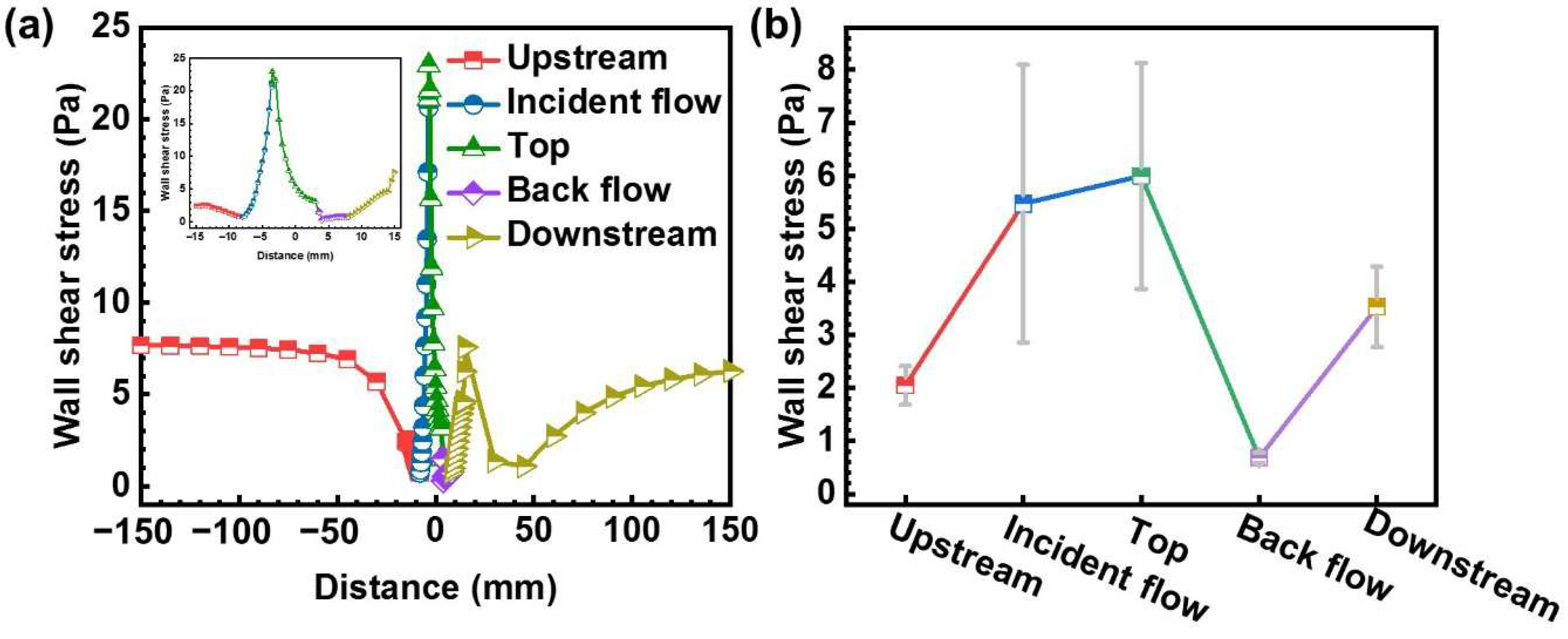
4.2. Shear Stress Effect

In addition to the mass transfer, the WSS also has a great effect on the corrosion process [12]. It can destroy the integrity of the corrosion products film mechanically.
WSS ( τ ) at the interface of WE/electrolyte solution can be expressed as [12]:
τ = μ d u d y
where, d u d y is the velocity gradient at the vertical distance y from the wall. It can be observed that the WSS is highly dependent on the flow velocity distribution.
The WSS of single-phase in the square channel can also be expressed as [30]:
τ = 1 2 ρ C f u 2
where C f is the fanning factor ( C f = 0.0376 Re 1 / 6 for channel flow).
The contour of WSS near the WRH wall is shown in Figure 14. WSS increases first until it reaches the maximum near the top surface and then decreases downstream. This trend is similar to the general variation of flow velocity along flow direction in Figure 13a. The WSS variations along the monitoring line and on the sample surfaces are plotted in Figure 15a and Figure 15b, respectively. It can be seen that the WSS of the top surface is the maximum, while that of the backflow surface is the minimum (Figure 15b). In general, the WSS on incident flow and top surfaces is larger than that of the other three surfaces.
The WSS increases in the sequence of the upstream surface, incident flow surface, and top surface. This trend is opposite to that of the pit number (Figure 11). Therefore, it can be deduced that the WSS can inhibit the formation of the pit. The pit often develops under corrosion products [45,55]. While high WSS does not facilitate the adherence of corrosion products [12,13,56]. Therefore, it can explain why the corrosion is retarded by increasing the WSS. Moreover, no great difference can be observed between the pit profile and the maximum depth of the samples (Figure 12). It suggests a weak relation between the WSS and the pitting appearance. All surfaces around WRH are dominated by pitting with similar profiles (Figure 8, Figure 10 and Figure 12). As a result, it is reasonable to conclude that the WSS does not affect the pit corrosion once the pit forms.
For the backflow and downstream surfaces, the pit number increases (Figure 10) with the increasing WSS (Figure 15). It seems the inhibition effect of the WSS on the pitting disappears because the WSS stays in a low-value region on the backflow surface and the downstream surface (Figure 15). However, the WSS on the latter surface is slightly higher than that on the former surface. Corrosion products are more prone to adhere to the surface on the condition of low WSS [12,56]. Therefore, as aforementioned, the charge transfer and mass transfer dominate the corrosion process instead of WSS in the presence of corrosion products.

4.3. Formation and Development of Pitting under Different Flow Conditions

Pitting corrosion occurred firstly on the surface of low alloy steel resulting in the local acid environment in the pits. Acidic corrosion products formed at the interface between the sample and electrolyte solution and accumulated at the initial anodic site, which accelerated the local anodic dissolution [45]. It is the main cause of pitting initiation in the flow environment [45]. As the pits grow, the opening of the pits is covered with corrosion products (Figure 9 and Figure 10), which leads to further acidification in the pit. When stable pits are formed, areas below the corrosion product will be the main cathode location. The pits will continue to expand longitudinally.
In a flowing solution environment, local corrosion also spreads along the flow direction (Figure 9). Micro-turbulence will form due to the piles up of the corrosion products. It can accelerate the mass transfer and corrosion downstream of the crown of the corrosion products of pitting. Therefore, “comet tails” forms along the flow direction. The turbulence gradually moves away from the pit and loses energy, creating a narrow tail at the end of the trail [44]. Compact corrosion products (Figure 9a–c) on the high flow velocity surfaces inhibit the migration of electrolytes resulting in a shorter comet tail (Figure 8a–c). The loose corrosion products (Figure 9d,e) on the low flow velocity surfaces could not significantly inhibit electrolyte migration along the flow direction in the pits. Therefore, the comet tails on backflow and downstream surfaces are longer (Figure 8d,e).
The development of pits is determined by the complex actions of mass transfer, WSS, and corrosion products. Two regions can be divided according to the values of hydrodynamics: high-value and low-value regions. The former includes the incident flow and the top surfaces with high flow velocity and WSS, and the latter contains the upstream surface, backflow surface, and downstream surface with low flow velocity and WSS (Figure 13 and Figure 15). The number of pits varies with different flow field conditions.
In the high-value region, the incident flow surface and top surface with high flow velocity are more affected by high WSS. The flow velocity and WSS on the top surface are greater than on the incident flow surface (Figure 13, Figure 14 and Figure 15). Ion exchange is easier, and it is difficult to form major local acidification zones on the top surface with high flow velocity [12,57,58]. High WSS also destroys corrosion products, making it difficult for the primary pit to grow steadily. As a result, the top surface has higher corrosion resistance (Figure 6) and fewer pits (Figure 10b,c) than the upstream surface.
In contrast, in the low-value region, the upstream surface, backflow surface, and downstream surface with low flow velocity are almost unaffected by WSS (Figure 14 and Figure 15). The charge transfer may play more roles than the mass transfer in the pitting corrosion process in the presence of the corrosion products at low flow velocity (Figure 6 and Figure 7). The combined effect of the two processes contributes to the pit number increase (Figure 10a,d,e) and the corrosion development (Figure 7).

5. Conclusions

The corrosion behavior of WRH in the flowing solution was studied by the RDE apparatus. In-situ electrochemical tests, surface characterization, and CFD simulation were combined to explain the correlation between the geometry of the WRH and the flow corrosion. The conclusions are as follows:
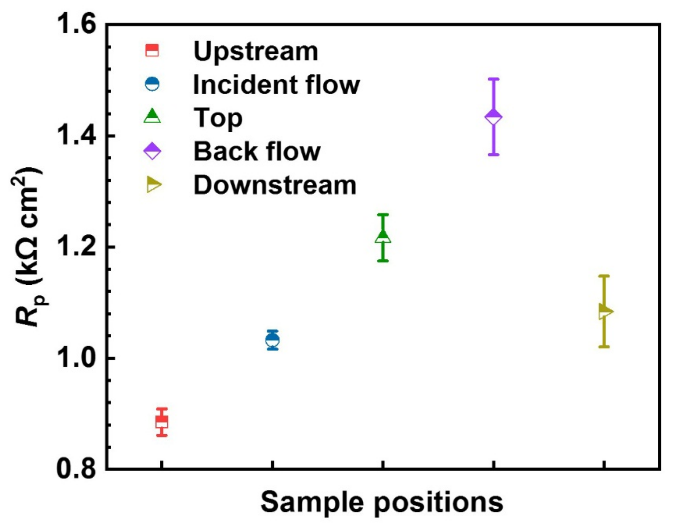
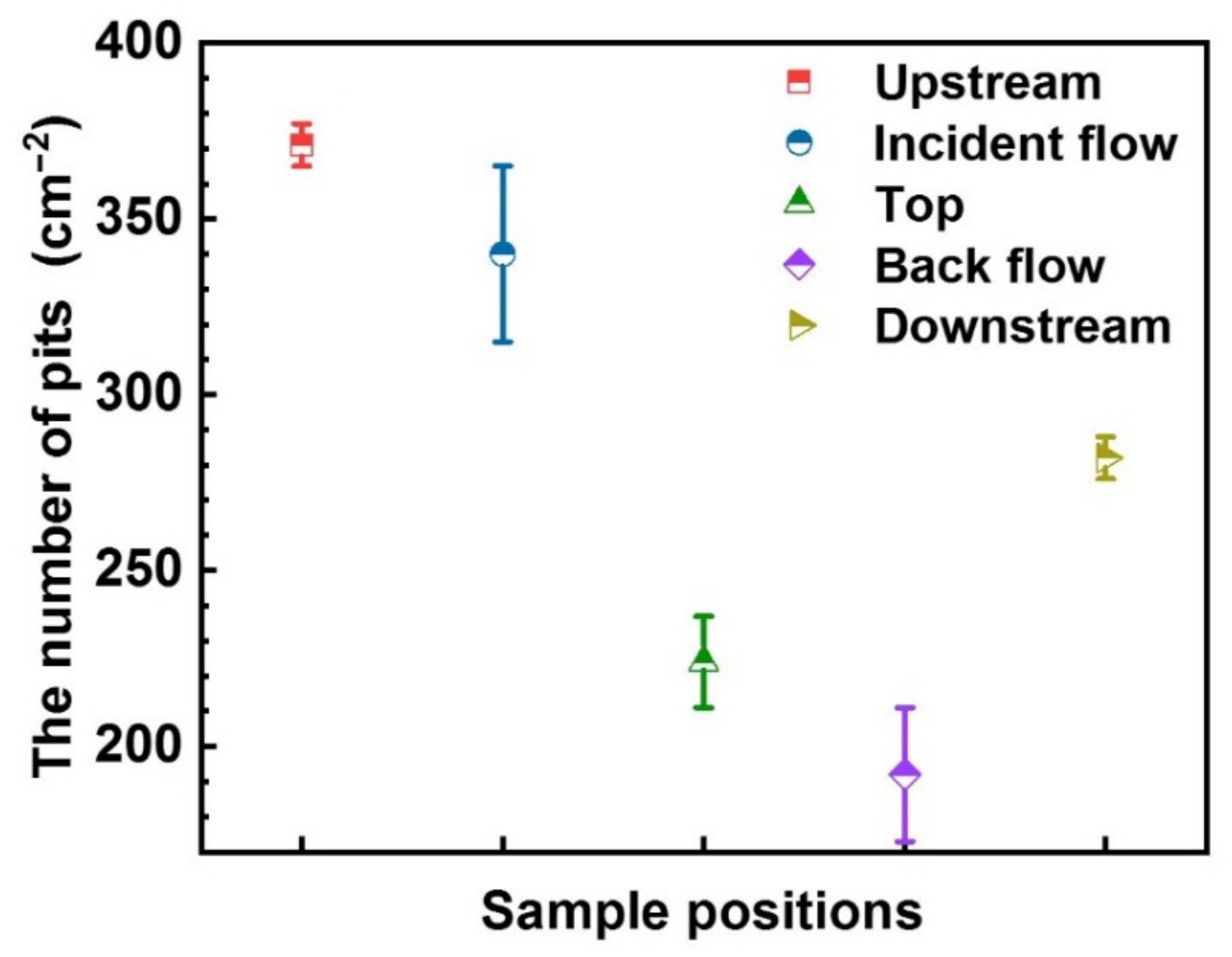
  • Pitting corrosion prevails on all the surfaces around the WRH. The number of pits is consistent with the 1/Rp in the decline sequence of the upstream surface, incident flow surface, downstream surface, top surface, and backflow surface.
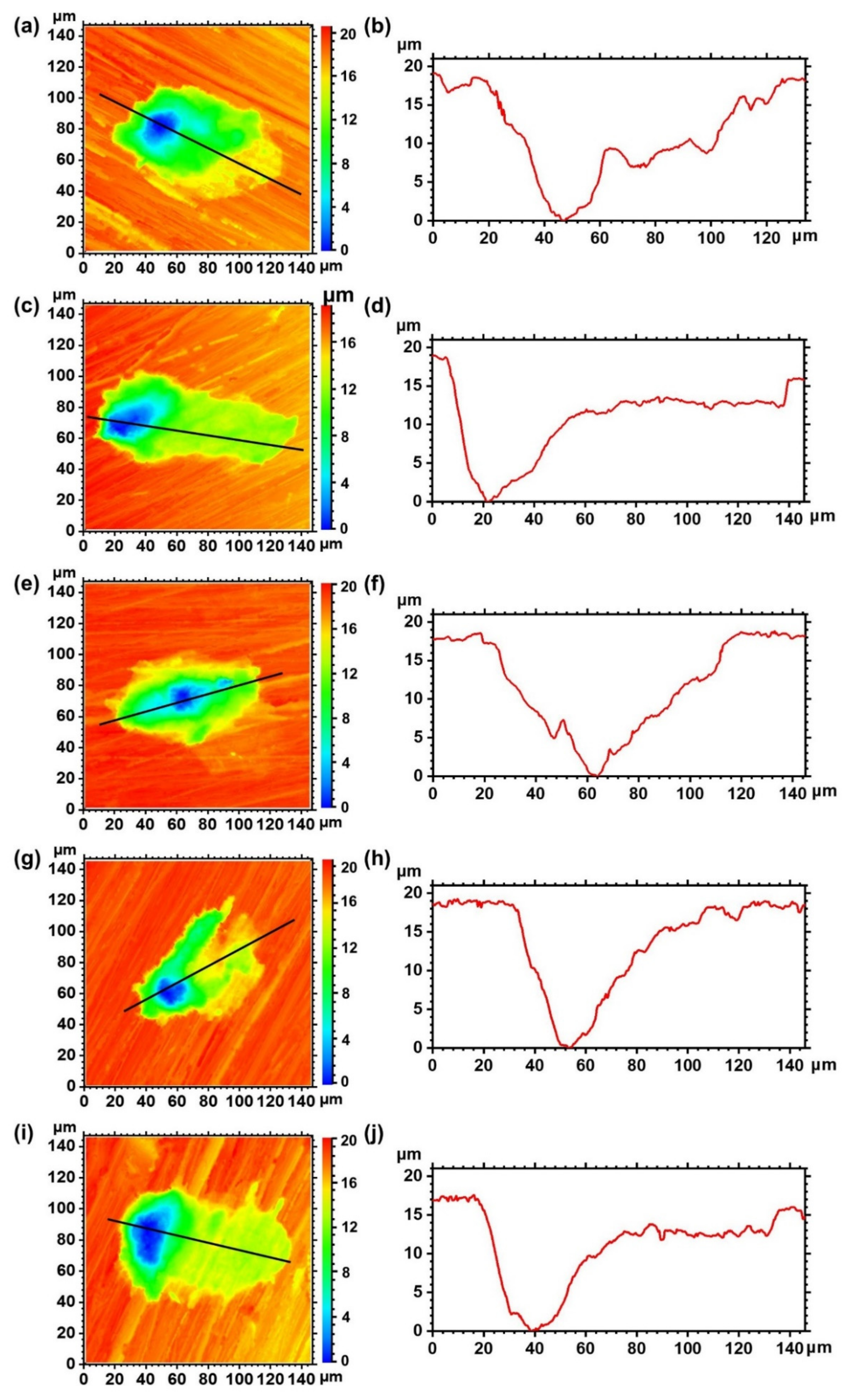
  • Local hydrodynamics affect the number of pits on the surfaces instead of the maximum pit depth and the profile.
  • On the incident flow surface and the top surface of WRH, high WSS inhibits the pitting, while for the other surfaces, the corrosion is almost unaffected by WSS.
  • Flow velocity and mass transfer are found to be not the only parameters determining the corrosion rate of local places of WRH. They should be cautiously considered when predicting corrosion in the presence of corrosion products.

Author Contributions

Conceptualization, K.Z., H.H. and Y.Z.; methodology, K.Z. and H.H.; validation, K.Z., H.H., Z.W., Y.Z., L.Z. and X.S.; formal analysis, K.Z. and H.H.; investigation, K.Z., Z.W. and L.Z.; re-sources, Y.Z.; data curation, K.Z.; writing—original draft preparation, K.Z.; writing—review and editing, H.H. and Z.W.; supervision, H.H., Y.Z., L.Z. and X.S.; project administration, H.H.; funding acquisition, L.Z. and X.S. All authors have read and agreed to the published version of the manuscript.

Funding

This research was funded by the National Natural Science Foundation of China (51971229) and the opening project of CAS Key Laboratory of Nuclear Materials and Safety Assessment (2021NMSAKF03).

Data Availability Statement

The raw/processed data required to reproduce these findings cannot be shared at this time as the data also forms part of an ongoing study. The data would be made available by the corresponding authors upon request.

Acknowledgments

The authors would like to acknowledge the financial support of the National Natural Science Foundation of China (51971229) and the opening project of CAS Key Laboratory of Nuclear Materials and Safety Assessment (2021NMSAKF03).

Conflicts of Interest

The authors declare no conflict of interest.

References

  1. Jiang, X.; Zheng, Y.; Ke, W. Effect of flow velocity and entrained sand on inhibition performances of two inhibitors for CO2 corrosion of N80 steel in 3% NaCl solution. Corros. Sci. 2005, 47, 2636–2658. [Google Scholar] [CrossRef]
  2. Ortega-Toledo, D.; Gonzalez-Rodriguez, J.; Casales, M.; Martinez, L.; Martinez-Villafañe, A. CO2 corrosion inhibition of X-120 pipeline steel by a modified imidazoline under flow conditions. Corros. Sci. 2011, 53, 3780–3787. [Google Scholar] [CrossRef]
  3. Zhang, G.; Zeng, L.; Huang, H.; Guo, X. A study of flow accelerated corrosion at elbow of carbon steel pipeline by array electrode and computational fluid dynamics simulation. Corros. Sci. 2013, 77, 334–341. [Google Scholar] [CrossRef]
  4. Wang, Z.; Zheng, Y. Critical flow velocity phenomenon in erosion-corrosion of pipelines: Determination methods, mechanisms and applications. J. Pipeline Sci. Eng. 2021, 1, 63–73. [Google Scholar] [CrossRef]
  5. Kim, S.-T.; Lee, I.-S.; Kim, J.-S.; Jang, S.-H.; Park, Y.-S.; Kim, K.-T.; Kim, Y.-S. Investigation of the localized corrosion associated with phase transformation of tube-to-tube sheet welds of hyper duplex stainless steel in acidified chloride environments. Corros. Sci. 2012, 64, 164–173. [Google Scholar] [CrossRef]
  6. Wu, W.; Hu, S.; Shen, J. Microstructure, mechanical properties and corrosion behavior of laser welded dissimilar joints between ferritic stainless steel and carbon steel. Mater. Des. 2015, 65, 855–861. [Google Scholar] [CrossRef]
  7. Okonkwo, B.O.; Ming, H.; Zhang, Z.; Wang, J.; Rahimi, E.; Hosseinpour, S.; Davoodi, A. Microscale investigation of the correlation between microstructure and galvanic corrosion of low alloy steel A508 and its welded 309/308L stainless steel overlayer. Corros. Sci. 2019, 154, 49–60. [Google Scholar] [CrossRef]
  8. Xu, L.; Zhang, J.; Han, Y.; Zhao, L.; Jing, H. Insights into the intergranular corrosion of overlay welded joints of X65-Inconel 625 clad pipe and its relationship to damage penetration. Corros. Sci. 2019, 160, 108169. [Google Scholar] [CrossRef]
  9. Rizk, T.; Thompson, G.; Dawson, J. Mass transfer enhancement associated with sudden flow expansion. Corros. Sci. 1996, 38, 1801–1814. [Google Scholar] [CrossRef]
  10. Owen, J.; Godfrey, J.; Ma, W.; de Boer, G.; Al-Khateeb, M.; Thompson, H.; Neville, A.; Ramsey, C.; Barker, R. An experimental and numerical investigation of CO2 corrosion in a rapid expansion pipe geometry. Corros. Sci. 2020, 165, 108362. [Google Scholar] [CrossRef]
  11. Zhong, X.; Shang, T.; Zhang, C.; Hu, J.; Zhang, Z.; Zhang, Q.; Yuan, X.; Hou, D.; Zeng, D.; Shi, T. In situ study of flow accelerated corrosion and its mitigation at different locations of a gradual contraction of N80 steel. J. Alloys Compd. 2020, 824, 153947. [Google Scholar] [CrossRef]
  12. Tan, Z.; Zhang, D.; Yang, L.; Wang, Z.; Cheng, F.; Zhang, M.; Jin, Y.; Zhu, S. Development mechanism of local corrosion pit in X80 pipeline steel under flow conditions. Tribol. Int. 2020, 146, 106145. [Google Scholar] [CrossRef]
  13. Zhang, D.; Yang, L.; Tan, Z.; Xing, S.; Bai, S.; Wei, E.; Tang, X.; Jin, Y. Corrosion behavior of X65 steel at different depths of pitting defects under local flow conditions. Exp. Therm. Fluid Sci. 2021, 124, 110333. [Google Scholar] [CrossRef]
  14. Ahmed, W.H.; Bello, M.M.; El Nakla, M.; Al Sarkhi, A. Flow and mass transfer downstream of an orifice under flow accelerated corrosion conditions. Nucl. Eng. Des. 2012, 252, 52–67. [Google Scholar] [CrossRef]
  15. Yamagata, T.; Ito, A.; Sato, Y.; Fujisawa, N. Experimental and numerical studies on mass transfer characteristics behind an orifice in a circular pipe for application to pipe-wall thinning. Exp. Therm. Fluid Sci. 2014, 52, 239–247. [Google Scholar] [CrossRef]
  16. Zheng, Y.; Kim, J.; Kim, I. A Study on Flow-accelerated corrosion of SA106 Gr.C weldment. J. Korean Weld. Soc. 2001, 19, 334–341. [Google Scholar]
  17. Barker, R.; Hu, X.; Neville, A. The influence of high shear and sand impingement on preferential weld corrosion of carbon steel pipework in CO2-saturated environments. Tribol. Int. 2013, 68, 17–25. [Google Scholar] [CrossRef]
  18. Shirinzadeh-Dastgiri, M.; Mohammadi, J.; Behnamian, Y.; Eghlimi, A.; Mostafaei, A. Metallurgical investigations and corrosion behavior of failed weld joint in AISI 1518 low carbon steel pipeline. Eng. Failure Anal. 2015, 53, 78–96. [Google Scholar] [CrossRef]
  19. Zeng, L.; Shuang, S.; Guo, X.; Zhang, G. Erosion-corrosion of stainless steel at different locations of a 90° elbow. Corros. Sci. 2016, 111, 72–83. [Google Scholar] [CrossRef]
  20. Owen, J.; Ducker, E.; Huggan, M.; Ramsey, C.; Neville, A.; Barker, R. Design of an elbow for integrated gravimetric, electrochemical and acoustic emission measurements in erosion-corrosion pipe flow environments. Wear 2019, 428–429, 76–84. [Google Scholar] [CrossRef]
  21. Xu, Y.; Tan, M. Visualising the dynamic processes of flow accelerated corrosion and erosion corrosion using an electrochemically integrated electrode array. Corros. Sci. 2018, 139, 438–443. [Google Scholar] [CrossRef]
  22. Xu, Y.; Tan, M. Probing the initiation and propagation processes of flow accelerated corrosion and erosion corrosion under simulated turbulent flow conditions. Corros. Sci. 2019, 151, 163–174. [Google Scholar] [CrossRef]
  23. Tomarov, G.V.; Lovchev, V.N.; Gutsev, D.F.; Shipkov, A.A.; Golubeva, T.N.; Greblov, P.N. Problems concerned with local erosion-corrosion of welded connections in the pipelines of a power unit at a nuclear power station. Therm. Eng. 2012, 59, 628–636. [Google Scholar] [CrossRef]
  24. Hosseini, F.; Isfahani, A.M.; Emami, M.D.; Mohseni, E. The effect of excessive penetration of welding on sand erosion pattern due to high speed gas-solid flows in elbows and reducers. Eng. Fail. Anal. 2022, 131, 105902. [Google Scholar] [CrossRef]
  25. Satoh, T.; Shao, Y.; Cook, W.G.; Lister, D.H.; Uchida, S. Flow-assisted corrosion of carbon steel under neutral water conditions. Corrosion 2007, 63, 770–780. [Google Scholar] [CrossRef]
  26. Fujiwara, K.; Domae, M.; Yoneda, K.; Inada, F. Model of physico-chemical effect on flow accelerated corrosion in power plant. Corros. Sci. 2011, 53, 3526–3533. [Google Scholar] [CrossRef]
  27. Wang, J.R.; Shirazi, S.A. A CFD based correlation for mass transfer coefficient in elbows. Int. J. Heat Mass Transf. 2001, 44, 1817–1822. [Google Scholar] [CrossRef]
  28. Zhang, G.; Cheng, Y. Electrochemical characterization and computational fluid dynamics simulation of flow-accelerated corrosion of X65 steel in a CO2-saturated oilfield formation water. Corros. Sci. 2010, 52, 2716–2724. [Google Scholar] [CrossRef]
  29. Ige, O.; Umoru, L. Effects of shear stress on the erosion-corrosion behaviour of X-65 carbon steel: A combined mass-loss and profilometry study. Tribol. Int. 2016, 94, 155–164. [Google Scholar] [CrossRef]
  30. Li, W.; Pots, B.; Brown, B.; Kee, K.E.; Nesic, S. A direct measurement of wall shear stress in multiphase flow-Is it an important parameter in CO2 corrosion of carbon steel pipelines? Corros. Sci. 2016, 110, 35–45. [Google Scholar] [CrossRef]
  31. Zheng, Y.; Yang, S.; Ling, X. Creep life prediction of small punch creep testing specimens for service-exposed Cr5Mo using the theta-projection method. Eng. Failure Anal. 2017, 72, 58–66. [Google Scholar] [CrossRef]
  32. Chen, Z.; Hu, H.; Zheng, Y.; Guo, X. Effect of groove microstructure on slurry erosion in the liquid-solid two-phase flow. Wear 2021, 466-467, 203561. [Google Scholar] [CrossRef]
  33. Chen, Z.; Hu, H.; Guo, X.; Zheng, Y. Effect of groove depth on the slurry erosion of V-shaped grooved surfaces. Wear 2022, 488-489, 204133. [Google Scholar] [CrossRef]
  34. EN ISO 5817:2014; Welding-Fusion-Weld Joints in Steel, Nickel, Titanium and Their Alloys (Beam Welding Excluded)-Quality Levels for Imperfectins. ISO: Brussels, Belgium, 2014.
  35. Zeng, L.; Zhang, G.; Guo, X. Erosion-corrosion at different locations of X65 carbon steel elbow. Corros. Sci. 2014, 85, 318–330. [Google Scholar] [CrossRef]
  36. Zeng, L.; Zhang, G.; Guo, X.; Chai, C. Inhibition effect of thioureidoimidazoline inhibitor for the flow accelerated corrosion of an elbow. Corros. Sci. 2015, 90, 202–215. [Google Scholar] [CrossRef]
  37. Yang, J.; Wang, Z.; Qiao, Y.; Zheng, Y. Synergistic effects of deposits and sulfate reducing bacteria on the corrosion of carbon steel. Corros. Sci. 2022, 199, 110210. [Google Scholar] [CrossRef]
  38. Zheng, K.; Hu, H.; Chen, F.; Zheng, Y. Failure analysis of the blackwater regulating valve in the coal chemical industry. Eng. Failure Anal. 2021, 125, 105442. [Google Scholar] [CrossRef]
  39. Zhang, G.; Cheng, Y. On the fundamentals of electrochemical corrosion of X65 steel in CO2-containing formation water in the presence of acetic acid in petroleum production. Corros. Sci. 2009, 51, 87–94. [Google Scholar] [CrossRef]
  40. Tang, Y.B.; Shen, X.W.; Liu, Z.H.; Qiao, Y.X.; Yang, L.L.; Lu, D.H.; Zou, J.S.; Xu, J. Corrosion Behaviors of Selective Laser Melted Inconel 718 Alloy in NaOH Solution. Acta Metall. Sin. 2022, 58, 324–333. [Google Scholar]
  41. Zhang, G.; Cheng, Y. Micro-electrochemical characterization of corrosion of welded X70 pipeline steel in near-neutral pH solution. Corros. Sci. 2009, 51, 1714–1724. [Google Scholar] [CrossRef]
  42. Wang, Z.; Hu, H.; Zheng, Y.; Ke, W.; Qiao, Y. Comparison of the corrosion behavior of pure titanium and its alloys in fluoride-containing sulfuric acid. Corros. Sci. 2016, 103, 50–65. [Google Scholar] [CrossRef]
  43. Pang, L.; Wang, Z.; Zheng, Y.; Lai, X.; Han, X. On the localised corrosion of carbon steel induced by the in-situ local damage of porous corrosion products. J. Mater. Sci. Technol. 2020, 54, 95–104. [Google Scholar] [CrossRef]
  44. Wharton, J.; Wood, R. Influence of flow conditions on the corrosion of AISI 304L stainless steel. Wear 2004, 256, 525–536. [Google Scholar] [CrossRef]
  45. Xu, Y.; Zhang, Q.; Zhou, Q.; Gao, S.; Bin Wang, B.; Wang, X.; Huang, Y. Flow accelerated corrosion and erosion-corrosion behavior of marine carbon steel in natural seawater. NPJ Mater. Degrad. 2021, 5, 1–3. [Google Scholar] [CrossRef]
  46. Zheng, R.; Zhao, X.; Dong, L.; Liu, G.; Huang, Y.; Xu, Y. On the cavitation erosion-corrosion of pipeline steel at different locations of Venturi pipe. Eng. Fail. Anal. 2022, 138, 106333. [Google Scholar] [CrossRef]
  47. Efird, K.D. Jet Impingement Testing for Flow Accelerated Corrosion; NACE International: Orlando, FL, USA, 2000. [Google Scholar]
  48. Gulbrandsen, E.; Grana, A. Testing of carbon dioxide corrosion inhibitor performance at high flow velocities in jet impingement geometry. Effects of Mass Transfer and Flow Forces. Corrosion 2007, 63, 1009–1020. [Google Scholar] [CrossRef]
  49. Halvorsen, A.; Sontvedt, T. CO2 Corrosion Model for Carbon Steel Including Wall Shear Stress Model for Multiphase Flow and Limits for Production Rate to Avoid Mesa Attack; NACE International: San Antonio, TX, USA, 1999. [Google Scholar]
  50. Nesic, S.; Solvi, G.T.; Enerhaug, J. Comparison of the rotating cylinder and pipe flow tests for flow-sensitive carbon dioxide corrosion. Corrosion 2012, 51, 773–786. [Google Scholar] [CrossRef]
  51. Poulson, B. Advances in understanding hydrodynamic effects on corrosion. Corros. Sci. 1993, 35, 655–665. [Google Scholar] [CrossRef]
  52. Nesic, S.; Postlethwaite, J.; Olsen, S. An electrochemical model for prediction of corrosion of mild steel in aqueous carbon dioxide solutions. Corrosion 1996, 52, 280–294. [Google Scholar] [CrossRef]
  53. Silverman, D.C. The rotating cylinder electrode for examining velocity-sensitive corrosion-A review. Corrosion 2004, 60, 1003–1023. [Google Scholar] [CrossRef]
  54. Silverman, C. Rotating cylinder electrode-geometry relationships for prediction of velocity-sensitive corrosion. Corrosion 1988, 44, 42–49. [Google Scholar] [CrossRef]
  55. Wang, Z.B.; Pang, L.; Zheng, Y.G. A review on under-deposit corrosion of pipelines in oil and gas fields: Testing methods, corrosion mechanisms and mitigation strategies. Corros. Commu. 2022, 7, 70–81. [Google Scholar] [CrossRef]
  56. Tan, Z.W.; Yang, L.Y.; Zhang, D.L.; Wang, Z.B.; Cheng, F.; Zhang, M.; Jin, Y.H. Development mechanism of internal local corrosion of X80 pipeline steel. J. Mater. Sci. Technol. 2020, 49, 186–201. [Google Scholar] [CrossRef]
  57. Li, L.; Wang, Z.; Zheng, Y. Interaction between pitting corrosion and critical flow velocity for erosion-corrosion of 304 stainless steel under jet slurry impingement. Corros. Sci. 2019, 158, 108084. [Google Scholar] [CrossRef]
  58. Zheng, Z.-B.; Long, J.; Guo, Y.; Li, H.; Zheng, K.-H.; Qiao, Y.-X. Corrosion and impact-abrasion-corrosion behaviors of quenching-tempering martensitic Fe-Cr alloy steels. J. Iron Steel Res. Int. 2022, 29, 1853–1863. [Google Scholar] [CrossRef]
Figure 1. Metallographic structure of 1Cr5Mo steel after etching.
Metals 13 00103 g001
Figure 2. Schematic diagram of RDE test system: (1) motor, (2) carbon brush, (3) copper ring, (4) graphite rod, (5) reference electrode, (6) salt bridge, (7) solution tank, (8) baffle, (9) specimen, (10) copper wire, (11) rotating disk, (12) solution tank holder, and (13) solution.
Metals 13 00103 g002
Figure 3. The sketch map of (a) the rotating disk with the samples on the (u1) upstream surface, (i2) incident flow surface, (t3) top surface, (b4) backflow surface, and (d5) downstream surface of the WRH, the size of (b) the trapezoidal protrusions with the skeleton map of the sample locations and (c) the electrochemical sample consisting of (1) specimen, (2) epoxy and (3) copper wire.
Metals 13 00103 g003
Figure 4. (a) CFD geometry model for simulating fluid flow near WRH in the square channel and sectional dimensions of (b) square channel and (c) trapezoidal bulge.
Metals 13 00103 g004
Figure 5. (a) Mesh sensitivity study of the flow velocity distribution on the monitoring line with hexahedral cells number 92,780, 287,160, 656,640, and 1,002,855, respectively. (b) Meshes selected in the final simulation of the flow domain.
Metals 13 00103 g005
Figure 6. EIS and the fitted curves of samples in different surfaces of WRH during the corrosion in RDE with a sinusoidal alternating amplitude of 10 mV and the frequency range from 10,000 Hz to 0.1 Hz: (a) Nyquist plots and (b) Bode plots.
Metals 13 00103 g006
Figure 7. The polarization resistance (Rp) of each sample on different WRH planes in the solution with a flow velocity of 2.3 m/s.
Metals 13 00103 g007
Figure 8. SEM corrosion morphologies of the samples located on (a) upstream surface, (b) incident flow surface, (c) top surface, (d) backflow surface, and (e) downstream surface of the WRH with corrosion products after 6 h flow corrosion.
Metals 13 00103 g008
Figure 9. SEM morphologies and elemental X-ray mapping of (a) the upstream surface, (b) incident flow surface, (c) top surface, (d) backflow surface, and (e) downstream surface of the WRH with corrosion products after 6 h flow corrosion.
Metals 13 00103 g009
Figure 10. OM corrosion morphologies of the samples on (a) upstream surface, (b) incident flow surface, (c) top surface, (d) backflow surface, and (e) downstream surface of the WRH without corrosion products after 6 h flow corrosion.
Metals 13 00103 g010
Figure 11. The number of pits on each surface of the WRH after removing the corrosion product.
Metals 13 00103 g011
Figure 12. 2D projection images of the deepest corrosion pits on the samples in (a) upstream surface, (c) incident flow surface, (e) top surface, (g) backflow surface, and (i) downstream surface of the WRH after removing corrosion products. Images of (b), (d), (f), (h), and (j) are the profiles of the pits along the line crossing the pits in images (a), (c), (e), (g), and (i) respectively.
Metals 13 00103 g012
Figure 13. (a) Flow velocity contour around the WRH, (b) the location of the red line for monitoring the flow velocity distribution near the material surface, and (c) flow velocity variation at the red line in (b) near the WRH wall along the flow direction and (d) average flow velocity of samples in different surfaces of the WRH at the condition of the main flow velocity of 2.3 m/s.
Metals 13 00103 g013
Figure 14. The contour of WSS at the WRH wall at the main flow velocity of 2.3 m/s.
Metals 13 00103 g014
Figure 15. (a) Variations of the WSS on the samples at different positions in the flow direction and (b) average WSS of samples in different surfaces of the WRH at the condition of the main flow velocity of 2.3 m/s.
Metals 13 00103 g015
Table 1. Equivalent circuit fitting of EIS data of each surface of the WRH.
PositionsRs
(Ω cm2)
Rct
(Ω cm2)
Qdl
(μF cm−2)
n   χ 2 10 4  
Upstream surface3.64 ± 0.21834.55 ± 26.80364.65 ± 8.410.844.77
Incident flow surface3.63 ± 0.04951.25 ± 22.56322.85 ± 8.980.853.03
Top surface3.63 ± 0.121356.00 ± 53.74337.65 ± 39.240.836.95
Backflow surface3.74 ± 0.161648.00 ± 152.74294.55 ± 20.860.863.98
Downstream surface3.63 ± 0.06996.90 ± 55.30365.55 ± 17.610.843.74
Table 2. The EDS analysis of the areas shown in Figure 9.
PositionsFe (wt.%)Cr (wt.%)O (wt.%)
Upstream surface81.354.0211.31
Incident flow surface83.204.109.64
Top surface80.044.3511.65
Backflow surface86.414.576.39
Downstream surface81.114.489.92
Table 3. Depth of the maximum pits on each surface of the WRH after removing the corrosion product.
PositionsDepth (μm)
Upstream surface18.56 ± 1.03
Incident flow surface18.68 ± 1.91
Top surface17.85 ± 1.21
Backflow surface18.90 ± 0.40
Downstream surface18.67 ± 1.00
Disclaimer/Publisher’s Note: The statements, opinions and data contained in all publications are solely those of the individual author(s) and contributor(s) and not of MDPI and/or the editor(s). MDPI and/or the editor(s) disclaim responsibility for any injury to people or property resulting from any ideas, methods, instructions or products referred to in the content.

