Data-Driven Dynamic Simulations of Gold Extraction Which Incorporate Head Grade Distribution Statistics

Abstract

The Alhué mining district, Chile, is an example of a high-grade Au-Ag-Zn(-Pb) deposit with mineralized veins that contain variable amounts of copper sulfides, which are detrimental to the cyanidation process. Similar deposits can be found in the central zone of Chile, with polymetallic veins (Au, Ag, Cu, Pb, and Zn) that are related to subvolcanic intrusive events, the development of collapse calderas, and extensive hydrothermal alteration, such as Bronces de Petorca, the Chancón mining district and Cerro Cantillana; areas of the world with similar formations include the western United States and the Henan Province in central China, for example. Mineralogical variation can be managed within the metallurgical process by alternating its operational modes. The decision to switch between modes is governed by current and forecasted stockpile levels feeding into the process, according to a discrete rate simulation (DRS) framework that has now been developed to incorporate head grade data for gold. Customized simulations that incorporate probability distribution models using head grade have now been developed, following a statistical analysis based on data from the Alhué district. This study applies data-driven simulation modeling to represent standardized operational modes and their impact on the operational performance of gold extraction.

1. Introduction

1.1. Process Simulation within Mine Improvement Projects

Simulation frameworks are critical for decreasing the risk of mining improvement projects [1,2,3], including changes in processing strategy. For aging gold mines in particular, the process often continues to run according to longstanding guidelines and settings, even when the nature of the incoming feed has changed; in the case of Minera Florida, this has resulted in increases in cyanide consumption as increasing amounts of certain copper sulfides are entering the feed [2], as described below (Figure 1). The status quo tends to be maintained within aging mines because any substantial modification to the processing strategy is perceived as risky unless it is supported by metallurgical studies and potential pilot tests to obtain the necessary data to parametrize operational changes and possibly to justify equipment upgrades. Furthermore, these metallurgical studies require a budget (often tens of thousands of dollars) and a time-commitment of personnel, e.g., a special projects team and/or outside consultants. Gaining support from management for experimentation and piloting can be difficult, unless it is demonstrated that a team would know what to do with the data once obtaining it; this is a “chicken and the egg” problem.

Herein lies the value of extensible simulation frameworks. They can be developed initially to support broad ranges of realistic data [3,4], successively detailing those operational aspects that are the most critical for attaining support for metallurgical studies. In gold extraction [2,5,6], as with other metals [7,8,9,10], the framework usually encapsulates a mass balance, describing the incoming feed streams and outgoing product streams, as well as reagent consumption (such as cyanide in the case of gold, [2]) and other key performance indicators (KPI). From our experience, a static mass balance is usually insufficient to attain management support for metallurgical studies since operational risks are characterized by dynamic surging that would approach or exceed the system tolerances. Indeed, static mass balances do not allow for representations of dynamic surging. At Minera Florida, for example, the surging of problematic copper sulfides (especially bornite and chalcocite) causes dynamic spikes in cyanide consumption that cannot be adequately represented within a static mass balance [2].

Discrete rate simulation (DRS) is perhaps the simplest approach to encapsulate dynamic mass balances [1,2,5,6,7,8], from which the context-specific feed variations can be developed in phases so that the corresponding risks can be quantified, as well as opportunities for improvement. As will be described in Section 2.3, DRS is a particular type of discrete event simulation (DES) in which incoming and outgoing material flows undergo discrete jumps over the simulated timeline. Moreover, DES/DRS frameworks are extensible, i.e., they can be successively extended in response to concerns from management (Figure 2) through the incorporation of models, submodels, “subsubmodels”, etc. For example, if an existing gold mine experiences feeds that have an increasing portion of copper sulfides, there may be a case to build a flotation circuit that would produce a copper concentrate in parallel to the cyanidation process, but management would be uncertain about the partitioning criteria that would divide marginal ore into the flotation feed versus the cyanidation feed [11]; in this case, the DES/DRS framework can be extended with models using published data (see [11] and/or [12], for example), demonstrating the potential benefits of the processing upgrade, ideally so that management can approve a detailed metallurgical study to refine the model parameters with site-specific data. Supposing that the proposed metallurgical study is not approved due to a series of criticisms from management. These criticisms are taken as guidance for the next iteration of model development (Figure 2a), which is then integrated into the next version of the simulation.

1.2. Minera Florida

In the case of Minera Florida, located within Chile’s Alhué District, it has been observed that certain copper sulfides within the feeds, especially bornite Cu₅FeS₄, chalcocite Cu₂S, and tetrahedrite 4Cu₂S₄⋅Sb₂S₃, cause spikes in cyanide consumption [2]; these minerals are 100, 100, and 44% soluble in a 0.1% NaCN solution at 45 °C and are occasionally called cyanicidal, as opposed to chalcopyrite CuFeS₂, which is only 8% soluble [11]. As described in the previous work [2], the Alhué deposit is a high-grade Au-Ag-Zn(-Pb) system in which the veins exhibit mineralized gradients of base metal sulfides and are subject to faults that intersect the underground workings of the mine. Similar deposits can be found in the central zone of Chile, which hosts polymetallic veins (Au, Ag, Cu, Pb, and Zn) that are related to subvolcanic intrusive events, the development of collapsed calderas, and extensive hydrothermal alteration, and pre- and syn-tectonic structural controlled veins, such as those at Bronces de Petorca, the Chancón mining district, and Cerro Cantillana [13,14]. These deposits are comparable to occurrences in the Tintic district, Salt Lake City, Utah, in which the ore mineralogy contains galena, sphalerite, acanthite, argentite, tetrahedrite-tennantite, enargite, proustite, hessite, calaverite, native gold, native silver, and a wide variety of relatively uncommon copper-, lead-, silver-, and bismuth-bearing sulfosalt minerals [15]. As another example, the Xiaoshan gold–polymetallic veins located in the Henan Province, central China, contain varying amounts of pyrite, galena, sphalerite, arsenopyrite, electrum, native gold, and silver-bearing sulfides [16].

The faulting at Minera Florida (and presumably in similar mines) is such that, within a single drift, there can be tens of meters of low-cyanide-consuming (LCC) ore, interrupted by a few meters of high-cyanide-consuming (HCC) ore, followed by a long extent of LCC ore. The LCC and HCC ores can have dramatically different visible appearances along the drift walls and were therefore easily linked to the downstream requirement of increased cyanide. Figure 1 is a plot of operational data obtained from June 2020 to February 2021, showing the effect of the aforementioned cyanide-soluble copper (also known as “cyanicidal copper”). A linear or quadratic regression is not forthcoming due to the corrective actions of expert operators and metallurgists, with R² values of 42.51% and 43.65% respectively. However, a comparative Student t test (see [17] or similar) of the 929 points below 600 ppm cyanide-soluble copper, and the 41 points above 1200 ppm, gives over 99.99% statistical confidence that cyanide-soluble copper minerals are associated with spikes in cyanide requirements; in fact, the cyanide consumption can be roughly tripled on a per-tonne-of feed basis. Essentially, beyond ~600 ppm of cyanide-soluble copper, the system gets overwhelmed, causing surges in cyanide requirements, despite the metallurgical operators’ best efforts.

The analysis illustrated by Figure 1 merely confirms what was being observed by geologists and operators, but it is somewhat crude since it does not detail the dynamic responses of the operators and therefore does not adequately support the integration/standardization of these responses. However, it motivated the quantitative approach of Órdenes et al. [2], which could indeed represent dynamic operational responses, which itself was an adaptation of the more general DES/DRS framework of Navarra et al. [1]. Yet, although the framework successfully illustrated the spiking of cyanide consumption and was thus generally well-received, management questioned the “parametrizibility” of the model. From their perspective, the framework had only qualitatively captured the dynamical aspects of their operational challenge, whereas they had hoped for a statistical treatment that would be “in the same spirit” as the analysis of Figure 1, including hypothesis testing. The DES/DRS framework is ultimately a composition of probabilistic distributions, as described in Section 2.3; management would question how well these distributions could be (optimally) parametrized to best represent the actual real data from their process.

These interactions have been a confluence of interdisciplinary expertise, which established the following consensus:

• There are numerous process variables that ideally should be represented within the framework as probability distributions, rather than as fixed deterministic values;
• Process data must be used to determine which standard distributions are most representative and what their parameter values should be;
• In the context of Minera Florida, the process variable that is currently perceived to be the most important is the head grade of the incoming ore, measured in gold-equivalent ounces per ton.

The methods presented in Section 2 are of general interest for system simulation [18] and are applicable to the entire set of process variables identified by Minera Florida. The specific list is not explicitly given here in the interest of confidentiality but contains typical measures, such as base metal grades and acid potentials, which are a common concern throughout the gold industry [19,20]. To balance the interests of generality and confidentiality, the sample computations of Section 3 consider the parametrization of only the head grade distributions, and similar approaches can be used for other variables.

2. Methods

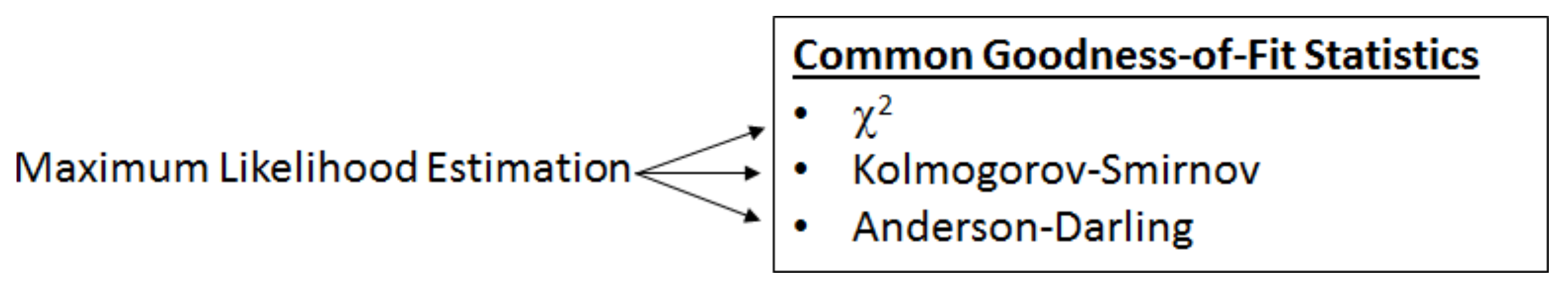
2.1. Maximum Likelihood Estimation of Distribution Parameters

Maximum likelihood estimation (MLE) is foundational to the data-driven parameterization of probability distributions [18,21] and precedes each of the goodness-of-fit (GOF) methods described in the following section (Figure 3). Supposing that a given set of numerical measurements, x₁, x₂, … x_n, follow a probability distribution, having density distribution f, MLE determines the parametrization of f that would have been the most likely to have produced said measurements.

Using standard notation, the probability density function (pdf) can be expressed as a function f(x) in which x is a possible value; by definition, ${{\displaystyle \int }}_{-\infty }^{\infty }f\left(x\right)$dx = 1. To explicitly cite the distribution parameters, we may write f(x|θ), in which θ is a tuple containing the list of parameters of the distribution. For example, a Gaussian distribution (also known as Normal distribution) can be expressed as f(x|μ,σ²), in which the parameters θ = (μ,σ²) are the mean and variance. MLE applies the principles of mathematical optimization and calculus to determine appropriate formulas (also known as “estimators”) for estimating parameter values, as a function of the observed values. In the case of a Gaussian distribution, the parameter values are commonly taken to be μ ≈ (Σ x_i/n) = $\overline{X}$ and σ² ≈ (Σ (x_i − $\overline{X}$)²/(n − 1)); however, industrial measurements of head grade and other process variables do not follow a Gaussian distribution, hence requiring the broader concepts of MLE and goodness-of-fit testing [18,22,23,24]. Especially for gold head grades, it is advised that the distribution of the grade be represented, rather than using averages to define a deterministically constant grade since the variation effects process decisions and outcomes. Moreover, it is important to implement a truly representative distribution since the erroneous usage of a Gaussian process can again effect process decisions and outcomes.

Anecdotally, professionals within the mining and metallurgical industries are reluctant to consider distributions other than the familiar Gaussian; they are often unfamiliar with the concepts of MLE and goodness-of-fit testing, unless they have had particular training in continuous improvement methodologies, such as Six-Sigma or related statistics or industrial engineering. The current treatment is intended to be adequately brief but self-contained. Alternatively, many practitioners are prone to using group averages to represent the plant behavior, which does not represent lost productivity from a sudden departure away from the operating tolerances or, in the case of gold processing, spikes in cyanide consumption.

Consider a series of random measurements: X₁, X₂, …, X_n, which are made and are found to have values of x₁, x₂, … x_n, and have some degree of precision: δ > 0. More explicitly, it has been found that X₁ ∈ [x₁ − ½δ, x₁ + ½δ] and X₂ ∈ [x₂ − ½δ, x₂ + ½δ], etc., and finally, that X_n ∈ [x_n − ½δ, x_n + ½δ] for a small value δ > 0. Supposing that these measurements follow a hypothetical distribution described by f, the probability that X₁ would have landed within the interval [x₁ − ½δ, x₁ + ½δ] is estimated by the area of a rectangle of width δ and height f(x₁), and similarly for the other measurements; hence, P(X₁ ∈ [x₁ − ½δ, x₁ + ½δ]) ≈ δ⋅f(x₁), P(X₂ ∈ [x₂ − ½δ, x₂ + ½δ]) ≈ δ⋅f(x₂), …, P(X_n ∈ [x_n − ½δ, x_n + ½δ]) ≈ δ⋅f(x_n). Assuming that the n samples are independent, the joint probability is given by the product:

$$P\left(X_1\in \left[x_1-½\mathsf{\delta },x_1+½\mathsf{\delta }\right], \dots ,X_n\in \left[x_n-½\mathsf{\delta },x_n+½\mathsf{\delta }\right]\right)\approx {\delta }^n{\displaystyle \prod }_{i=1}^{n}f\left(x_i\right)$$

(1)

MLE maximizes this joint probability by adjusting the parameters of f, asking the question: which parameter values would have maximized the probability of having measured X₁ ≈ x₁ and X₂ ≈ x₂ and … and X_n ≈ x_n?

Assuming that the degree of precision, δ, is sufficiently small, then it does not affect the maximization and can be ignored. Thus, as a proxy for the joint probability (Equation (1)), we define the likelihood L(x), in which x = (x₁,x₂,…x_n) is the tuple of measured values:

$$L\left(\mathit{x}\right)={\displaystyle \prod }_{i=1}^{n}f\left(x_i\right)$$

(2)

To explicitly cite the distribution parameters θ = (θ₁, θ₂, … θ_p), we write:

$$L\left(\mathit{x}|\mathit{\theta }\right)={\displaystyle \prod }_{i=1}^{n}f(x_i|\mathit{\theta })$$

(3)

It is common to maximize the natural logarithm of L, rather than L itself, which converts the product of Equation (3) into a summation. The log-likeliness function is thus given by:

$$l\left(\mathit{x}|\mathit{\theta }\right)={\displaystyle \sum }_{i=1}^n\ln \left(f(x_i|\mathit{\theta })\right)$$

(4)

and indeed, the maximization of l = ln (L), rather than L, does not change the result, considering that ln is a strictly increasing function. This transformation slightly simplifies the calculus to parameterize common distributions, such as the Gaussian and exponential [21].

Moreover, it is standard to use a “hat” to denote the MLE estimates, i.e., the $\widehat{\mathit{\theta }}=\left({\widehat{\theta }}_1,{\widehat{\theta }}_2,\dots ,{\widehat{\theta }}_p\right)$ are the particular values of θ = (θ₁, θ₂, … θ_p) that maximize the joint probability (or equivalently the likelihood or log-likelihood) of having measured X₁ ≈ x₁ and X₂ ≈ x₂ and … and X_n ≈ x_n. The MLE-parametrized density function is also denoted with a ”hat”, as in $\widehat{f}\left(x\right)=f\left(x|\widehat{\mathit{\theta }}\right)$, and similarly for the cumulative distribution function $F\left(x\right)={{\displaystyle \int }}_{-\infty }^{x}f\left(u\right)du$; the MLE-parameterization is expressed as $\widehat{F}\left(x\right)=F\left(x|\widehat{\mathit{\theta }}\right)={{\displaystyle \int }}_{-\infty }^{x}f\left(u|\widehat{\mathit{\theta }}\right)du$.

Depending on the distribution, there may be constraints on certain parameter values, e.g., only positive σ² values are allowed in the case of a Gaussian distribution. Therefore, the exercise of MLE is in general a constrained optimization:

$$\widehat{\mathit{\theta }}\left(\mathit{x}\right)=\underset{\mathit{\theta }\in \mathsf{\Theta }}{\mathrm{argmax}}L\left(\mathit{x}|\mathit{\theta }\right)=\underset{\mathbf{\theta }\in \mathsf{\Theta }}{\mathrm{argmax}}l\left(\mathit{x}|\mathit{\theta }\right)$$

(5)

in which Θ is the feasible parameter space, Θ ⊂ ℝ^p, yet there are many practical cases in which the constraints do not affect the optimization. In practice, Θ can be taken as ℝ^p to apply unconstrained optimization techniques (calculus), and only if the resulting parametrization is infeasible is it necessary to consider a specialized constrained approach.

If L(x|θ) varies continuously with θ, then elementary differential calculus can be applied. For distributions with only one parameter, $\widehat{\theta }$ is determined by setting ∂L/∂θ to zero and solving for θ. Nearly all of the distributions under consideration, regarding the Minera Florida data, consist of two parameters, in which case $\widehat{\mathit{\theta }}=\left({\widehat{\theta }}_1,{\widehat{\theta }}_2\right)$ is determined by setting ∂L/∂θ₁ = 0 and ∂L/∂θ₂ = 0 and solving for two unknowns: θ₁ and θ₂. More generally, for p-parameter distributions, the calculus consists of solving p equations to obtain p unknowns [21]. As will be described in Section 3.1, the gold head grades are best represented by a log-normal distribution, for which the MLE estimation formulas (also known as “estimators”) have been found to be:

$$\widehat{\mu }\left(\mathit{x}\right)=\frac{1}{n}{\displaystyle \sum }_{i=1}^n\ln x_i$$

(6)

$$\widehat{{\sigma }^2}\left(\mathit{x}\right)=\frac{1}{n}{\displaystyle \sum }_{i=1}^n{\left(\ln x_i-\left[\widehat{\mu }\left(\mathit{x}\right)\right]\right)}^2$$

(7)

Both expressed as a function of the observed measurement values, x, to emphasize that the parametrization is data-driven. Furthermore, it is data-driven in a dependable (rigorous) sense, i.e., the sense of maximum likeliness. Alternatively, for example, log-normal could be erroneously fitted with the logarithm of the mean, rather than the mean of the logarithm; the MLE formulation resolves these potential pitfalls.

However, prior to selecting a particular standard distribution to represent a particular variable (e.g., log-normal to represent the head grade), a litany of other potential distributions are also considered, which are each parameterized according to Equation (5), leading to distribution-specific estimation formulas (e.g., Equations (6) and (7) for the case of log-normal). 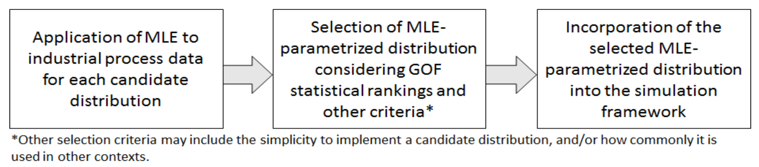The idea is to compare the best log-normal distribution to the best Gaussian distribution, and to the best Gamma distribution, and so on. In this case, “best” means optimally parametrized in the sense of MLE. The distribution-specific estimators are usually programmed within software such as the input analyzer that is available with Rockwell Arena or the commonly used easy fit by Math Wave Technologies. In typical applications, it may not be necessary to derive or to work directly with the distribution-specific estimation formulas, relying instead on the software; however, the detailing of the DES/DRS framework has required that we directly program these estimators as an essential part of the data processing (Figure 4). It is prudent (and strongly recommended) to derive the formulas for any of the MLE estimators that are programmed into such a framework to be precisely sure of what the parameters represent. These calculus exercises are fairly basic and avoid errors that would later be very difficult to detect. As an example, once again, Equation (5) demands the mean of the logarithm rather than the logarithm of the mean. Consider further that an unapologetically deterministic simulation may be preferred over such an ill-conceived probabilistic model that gives false confidence.

In summary, MLE is the rigorous mathematical basis for data-driven parameterization. It provides the formulas to channel industrial measurements into the DES/DRS framework of Órdenes et al. [2]. The approach and experience that we have gained in the context of Minera Florida can be adapted to other mining contexts.

2.2. Chi-Squared, Kolmogorov–Smirnov, and Anderson–Darling Statistics

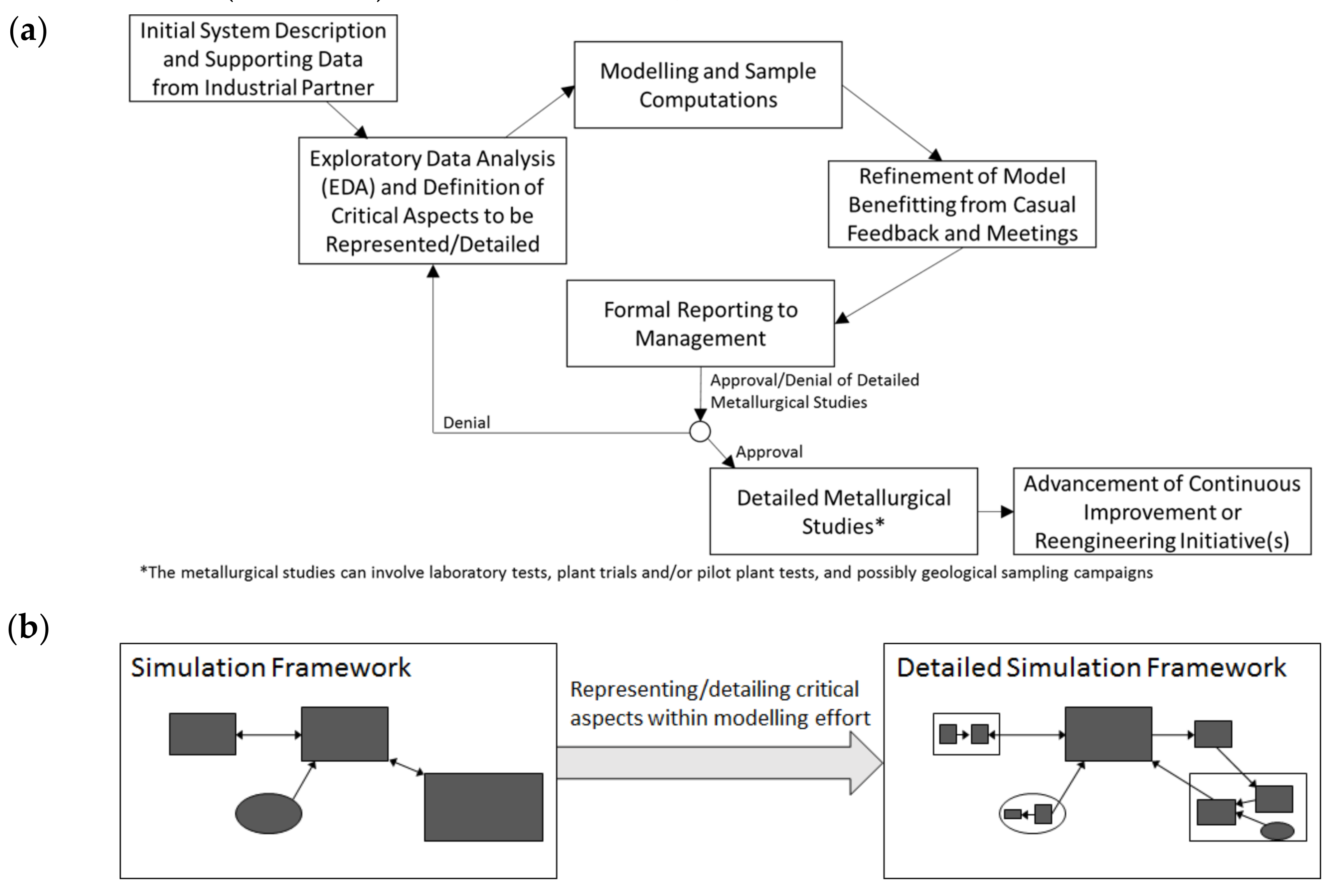
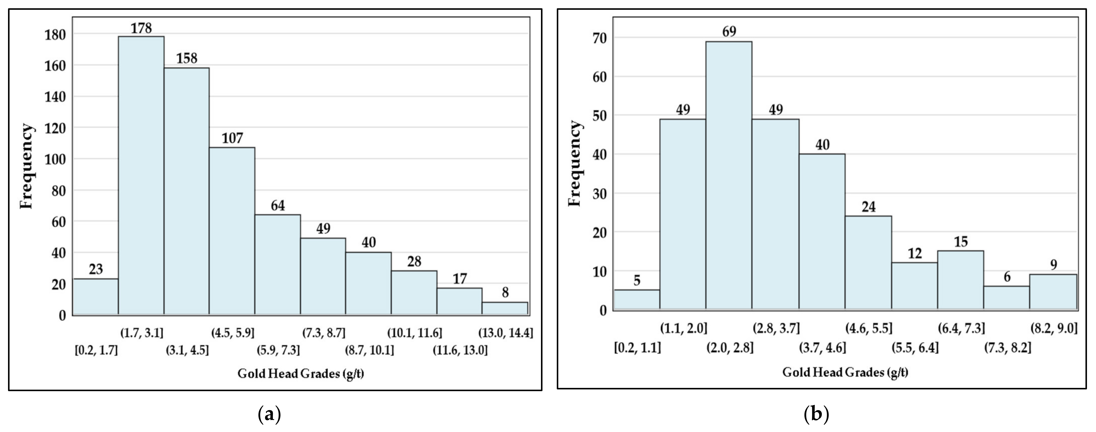
Critical process variables, such as gold head grade, can be observed with histograms and clearly do not follow Gaussian distributions. Yet, statistical concepts that are erroneously adapted to the Gaussian distributions are still commonly used. Even when metallurgical operators and engineers recognize this “non-Gaussianity”, they are left with the task of selecting other standard distributions which might be more appropriate, but without knowledge of a rigorous approach, the Gaussian distribution is nonetheless retained. This erroneous application of the Gaussian process makes it difficult to justify a budget for detailed metallurgical studies (Figure 2) and has hindered the progress at Mineral Florida. Particularly, in responding to critical variation, such as with gold head grade, any deterministic approach is inadequate, but an ill-adjusted probabilistic approach may be even less desirable since it provides false confidence.

In other industrial contexts, the typical approach is to rank the MLE parametrization for a list of candidate distributions according to goodness-of-fit (GOF) statistics (Figure 3). Given several hundred gold head grade measurements, for example, the preference to model these data as log-normal rather than as Gaussian involves a comparison of GOF metrics from the MLE-parameterized log-normal together with the GOF metrics of the MLE-parameterized Gaussian, with both parameterized with respect to the same given data. More broadly, software such as the Rockwell input analyzer and easy fit (of Math Wave Technologies) tabulate the GOF metrics for an extensive list of candidate distributions. The user of the software may then select the best-ranked distribution but, alternatively, may select another highly ranked distribution if it has fewer parameters and/or can be more effectively implemented or studied in computational experiments. This shall be further discussed below.

The chi-squared (χ²) is the most widely known statistic that is used for GOF. Indeed, the χ² is described in elementary statistics textbooks such as [20]. Anecdotally, practitioners of extractive metallurgy may have a vague familiarity with χ², possibly for the construction of variance intervals of Gaussian-distributed variables or embedded within ANOVA tables in the evaluation of the F statistics (that compares variances of Gaussian-distributed variables [25]). In its classic use as a GOF statistic (dating to 1900, [26]), it is evaluated as a weighted sum of squares over k categories:

$${\chi }^2={\displaystyle \sum }_{j=1}^k\left(\frac{1}{n_j^{\mathrm{Dist}}}\right){\left(n_j^{\mathrm{Obs}}-n_j^{\mathrm{Dist}}\right)}^2$$

(8)

in which $n_j^{\mathrm{Obs}}$ is the number of observed measurements that fall within category j, and $n_j^{\mathrm{Dist}}$ is the number of measurements predicted by the MLE-parametrized hypothetical distribution, noting that the $\frac{1}{n_j^{\mathrm{Dist}}}$ factors act as weighting; alterations of the classic χ² may consider different weightings. In general, according to Equation (8), distributions whose MLE-parametrization have smaller differences ($n_j^{\mathrm{Obs}}-n_j^{\mathrm{Dist}}$) over the k categories will give smaller ${\chi }^2$ values and are hence, a better fit.

One drawback of this use of chi-squared is the ambiguity in the definition of the k categories. Ad hoc approaches for evaluating discrete distributions are described in [22], including mergers of smaller categories resulting in larger categories that are adequately sampled and (ideally) are equiprobable. For continuous distributions such as Gaussian, log-normal, etc., the k categories correspond to a set of intervals, {(a_j−1,a_j]|j = 1… k}, and the equiprobable condition ($n_j^{\mathrm{Dist}}=\frac{n}{k}$) is strictly enforced by setting:

$$a_j={\widehat{F}}^{-1}\left(j/k\right)$$

(9)

in which ${\widehat{F}}^{-1}$ is the inverse of the MLE-parameterized cumulative distribution function. Thus, for continuous distributions, ${\chi }^2$ is expressed in terms of the number of samples n:

$${\chi }^2=\left(\frac{k}{n}\right){\displaystyle \sum }_{j=1}^k{\left(n_j^{\mathrm{Obs}}-\frac{n}{k}\right)}^2$$

(10)

Yet, even for continuous distributions, there is generally no optimal approach for fixing k since the optimal number of categories depends on the (unknown) distribution that underlies the data. A commonly used formula is

$$k=\lfloor 1+{\log }_{2}n\rfloor$$

(11)

which is applied in Section 3.1 for gold head grades.

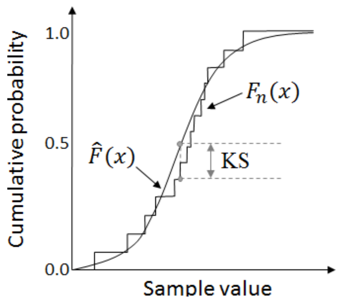
Alternatives to the χ² include Kolmogorov–Smirnov (KS) and Anderson–Darling (AD) statistics, both of which avoid the artificial construction of categories. KS and AD both make use of the empirical cumulative distribution,

$$F_n\left(x\right)=\frac{\left|\left\{x_1,x_2,\dots x_n\right\}\cap \left(-\infty ,x\right]\right|}{n}$$

(12)

F_n(x) is thus the portion of observed measurements whose value is smaller or equal to x, which forms a step function graph as illustrated in Figure 5. Herein the KS statistic is the largest absolute distance between $F_n$ and $\widehat{F}$. Formally:

$$\mathrm{KS}=\underset{x\in ℝ}{\sup }\left|F_n\left(x\right)-\widehat{F}\left(x\right)\right|$$

(13)

KS is an unweighted metric, i.e., there is no weighting w(x) that multiplies the absolute difference. A supremum operation (sup) is more appropriate than a maximum (max) to ensure the largest interpretation of $\left|F_n\left(x_i\right)-\widehat{F}\left(x_i\right)\right|$ when evaluating the distance at the sample points x_i, i.e., $\left|F_n\left(x_i\right)-\widehat{F}\left(x_i\right)\right|$ is taken to be the larger of either the left limit $\underset{x\to x_i{}^{-} }{\lim }\left|F_n\left(x\right)-\widehat{F}\left(x\right)\right|$ or the right limit $\underset{x\to x_i{}^{+}}{\lim }\left|F_n\left(x\right)-\widehat{F}\left(x\right)\right|$ [23].

The Anderson–Darling statistic is conceived as a weighted integral of the squared difference of $F_n$ and $\widehat{F}\left(x\right)$,

$$\mathrm{AD}=n{{\displaystyle \int }}_{-\infty }^{\infty }\frac{{\left(F_n\left(x\right)-\widehat{F}\left(x\right)\right)}^2}{\widehat{F}\left(x\right)\left(1-\widehat{F}\left(x\right)\right)}d\widehat{F}\left(x\right)$$

(14)

in which the weighting $\frac{1}{\widehat{F}\left(x\right)\left(1-\widehat{F}\left(x\right)\right)}$ preferentially penalizes the deviations in the tails; in practice, AD is indeed more sensitive to tail deviations than either the χ² or the KS. Through a partial fraction decomposition of the integrand and the articulation of $F_n$ as piecewise constant intervals, and a change of the integrating domain such that $d\widehat{F}\left(x\right)=\widehat{f}\left(x\right)dx$, Equation (14) is resolved as:

$$\mathrm{AD}=-n-\left(\frac{1}{n}\right){\displaystyle \sum }_{i=1}^n\left(2i-1\right)\left[\ln \widehat{F}\left(x_{\left(i\right)}\right)+\ln \left[1-\widehat{F}\left(x_{\left(n+1-i\right)}\right)\right]\right]$$

(15)

in which {x₍₁₎, x₍₂₎, … x_(n)} is the sorting of the sample data {x₁, x₂, … x_n} in ascending order, i.e., x₍₁₎ ≤ x₍₂₎ ≤ … ≤ x_(n).

In developing data-driven industrial simulations, the χ², KS, and AD statistics are used to rank the MLE-parametrized distributions, indicating which distributions are representative of the various process variables. However, they often provide conflicting results, including the χ² rankings, which can change depending on how the categories are constructed. Moreover, common software such as easy fit and the Rockwell input analyzer consider an extensive list of distributions, many of which are obscure. For example, the top-ranked distribution according to KS may be a Johnson S_U, which is a four-parameter transformation of the standard Gaussian; if a more commonly used distribution is nearly as good in KS ranking, and is also favorable in the χ² and AD rankings, then the more common distribution is a better choice. Firstly, the more common distributions are prolific in published studies across many disciplines, allowing for cross-disciplinary comparisons. More importantly, the common distributions are better received in preparation for detailed studies (Figure 2a) that would ultimately allow more detailed modelling; the fitted distributions that are most impactful to the simulation may (or should) ultimately be replaced by mechanistic models (Figure 2b). The application of an obscure multiparameter distribution may be counter-productive since either (1) the process variable is critical and should genuinely be represented through a submodel rather than an obscure distribution, or (2) the variable is not so critical and should rather be represented by a common distribution instead of being a point of unnecessary scrutiny for management.

An existing nuance is that the χ², KS, and AD rankings of MLE-parameterized distributions are descriptive in the sense of descriptive statistics; this is in contrast to inferential statistics, which relies on hypothesis testing to infer the properties of an underlying process, given a set of sample data. In the current context, it is understood that the process variables do not actually follow any of the idealized distributions listed by the fitting software; the task is to decide which of these distributions are best suited to argue for the next phase of simulation modelling, with the objective of efficiently directing the resources for further study (Figure 2) and ultimately for process improvement.

In a different context, whereby a systematic sweep of numerous candidate distributions is not involved, a GOF hypothesis test is applied when there is a hypothetical distribution that is specifically observed to be a possible description of the underlying process. For χ², KS, and AD tests, a null hypothesis is formulated as:

H₀. 

The measured sample data {x₁, x₂… x_n} follows a distribution whose cumulative probability function is described by F₀(x|θ) having parameters θ.

The observed χ², KS, and AD can then be computed by applying Equations (8), (13), or (15), respectively, to the MLE-parametrized hypothetical cumulative probability function ${\widehat{F}}_0$. For a significance level α ∈ (0, 1], the null hypothesis is rejected if the observed statistics exceed a critical value; such a rejection indicates a minimal confidence (1−α) level in which the underlying process does not follow the hypothetical distribution. For the χ² test, the test is formulated as:

$$\left({\chi }^2>{\chi }_{1-\alpha ,k-m}^2\right)\Rightarrow \left(\mathrm{Reject} H_0\right)$$

(16)

in which the critical value is ${\chi }_{1-\alpha ,k-m}^2$ can be obtained from textbooks or from software (Excel, Minitab, etc.) considering (k−p) degrees of freedom; p is the number of parameters within the hypothetical distribution, e.g., p = 2 for Gaussian and log-normal. The critical KS_1−α and AD_1−α are both distribution-specific [23,24] and consider multiplicative adjustment factors that depend on the number of samples n.

$$\left(\mathrm{KS}>{\varphi }_n^{\mathrm{KS}}{\mathrm{KS}}_{1-\alpha }\right)\Rightarrow \left(\mathrm{Reject} H_0\right)$$

(17)

$$\left(\mathrm{AD}>{\varphi }_n^{\mathrm{AD}}{\mathrm{AD}}_{1-\alpha }\right)\Rightarrow \left(\mathrm{Reject} H_0\right)$$

(18)

For a hypothetical Gaussian distribution, the adjustment factors are ${\varphi }_n^{\mathrm{KS}}=\left(\sqrt{n}-0.01+\frac{0.85}{\sqrt{n}}\right)$ and ${\varphi }_n^{\mathrm{AD}}=\left(1+\frac{4}{n}-\frac{25}{n^2}\right)$. For certain distributions, such as the exponential, the n-dependent adjustment includes an additive shift as well as a multiplicative factor [23]. Importantly for the gold head grades, the normality tests can be adapted to the log-normal simply by taking the logarithm of the sample data, y_i = ln (x_i), and then applying Equations (17) and (18) to {y₁, y₂, … y_n}. Section 3.1 applies the tests of Equations (16)–(18), with α = 0.05 to test log-normality.

It is indeed customary to apply the tests of Equations (16)–(18) for the selected distribution, which incidentally may not be the top-ranked of all GOF metrics. But particular caution is required when interpreting the rejection of these hypotheses, especially when communicating to management (Figure 2). In the descriptive statistical context of GOF ranking to support simulation modelling, the null hypothesis, H_0, is moot a priori unless there is a genuine expectation that the underlying process could follow the proposed distribution. The ultimate decision to accept a distribution-based representation of a process variable, or to replace it with a more detailed submodel (i.e., to truly reject the distribution), must depend on how significant the process variable is to the engineering decision-making. Otherwise, the tendency is to focus erroneously on irrelevant aspects of the model that justifiably have a large statistical deviation from the observed data; in practice, it is typical that the unimpactful aspects (as determined by the approach in Figure 2) of the model remain less developed in favor of the more impactful aspects that should indeed be more developed. Therefore, simulation modelers must understand the notion of inferential statistical significance, especially to distinguish it from engineering decision-making significance. It is likely that all distribution-based representations should ideally be replaced by submodels, “subsubmodels”, etc. (Figure 2b) from a statistical point-of-view with α ≈ 0. Yet, in practice, the budgetary and human resource limitations cause the modelling effort to prioritize those aspects which are truly critical to the advancement of the project (Figure 2a). This engineering-oriented prioritization is not reflected within the weightings of Equations (8), (13), and (14).

2.3. Supporting of Monte Carlo and DES/DRS Frameworks with Exploratory Data Analysis

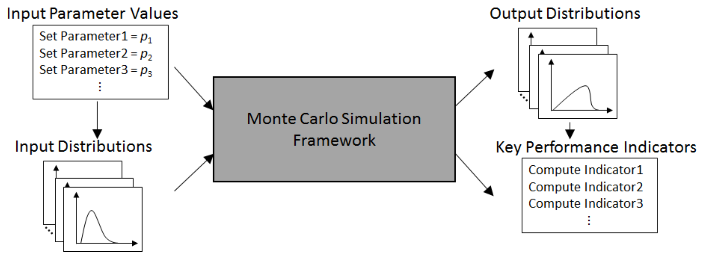
In broad terms, a Monte Carlo simulation framework considers:

• A set of input parameters that configure the system that is to be simulated;
• That one or more of the inputs are to be represented by probability distributions rather than deterministic values;
• That the execution of the simulation consists of numerous replicas, each based on an independent generation of random numbers following the input probability distributions;
• That the collection of outputs from the replicas approximate the distribution of possible system behaviors;
• Typically, the overall system performance can be assessed through the output distributions and quantified by so-called key performance indicators (KPIs).

Essentially, a Monte Carlo simulation uses random number generation (RNG) to convert input parameters and distributions into output distributions and KPIs. As illustrated in Figure 6, some of the input parameters can be used to parametrize the input distributions as well as for configuring the internal aspects of the framework. Similarly, certain KPIs can be drawn as summative evaluations of the output distributions, while others may be directly computed by the framework.

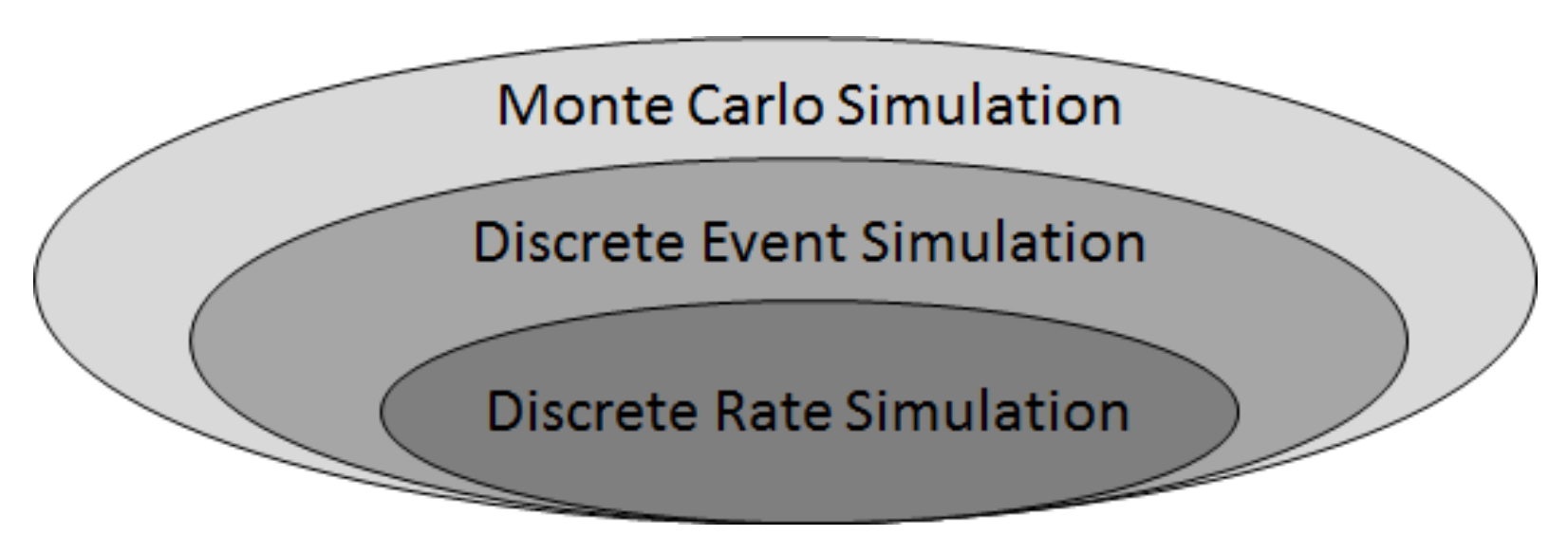
Moreover, a discrete event simulation (DES) framework represents a dynamic system via input parameters and distributions as well as a collection of state variables that are updated at discrete points along a simulated timeline, hence, discrete events. Indeed, it is the simulated clock jumps from one discrete event to the next without explicitly representing the behavior between the events. An activity or condition that extends over a duration is represented by a discrete event that signals its beginning and a later discrete event that signals its end; within this duration, there may be a series of discrete events, and possibly sub-activities, “sub-sub-activities”, etc. depending on the level of detail. DES models can therefore be developed in iterative phases that incorporate hierarchical complexity, as per Figure 2, which define additional state variables and incrementally detail the system’s activities, conditions, processes, etc. There are cases in which a purely deterministic DES may be of interest (e.g., for initial conception or later verification), but in practice, DES is seen as a type of Monte Carlo simulation (Figure 7), considering that the time between events can be the result of RNG and that the updating of state variables that occur at the events are generally the result of RNG.

Furthermore, a discrete rate simulation (DRS) is a particular kind of DES in which the state variables consist of pairs of levels and rates (l_j,r_j), and the discrete events consist of threshold crossings. Each level-rate pair represents a continuous variable that follows piecewise linear dynamics. The occurrence that such a continuous variable crosses a threshold is, itself, a discrete event (e.g., an ore stockpile level crossing below a critical value). When the ith threshold crossing event occurs at time t_i, the levels l_j are updated as per

$$l_j:=l_j+\left(t_i-t_{i-1}\right)r_j$$

(19)

and, subsequently, the corresponding rates, r_j, are updated by model-specific formulas for j ∈ {1,2…,n_CSV}, in which n_CSV is the number of continuous state variables. The model-specific updating of r_j can incorporate RNG, particularly in a mineral processing and extractive metallurgical context, when representing geological variation [1,2,6,7,8]. These rate updates can also be the result of an operational policy that depends on the current configuration of the plant, as well as current and forecasted stockpile levels. Also, depending on the particular event, there can also be discrete jumps in l_j as well as in r_j, for example, a corrective action can include an immediate injection of a certain reagent, as well as a change in the continuous feeding rate.

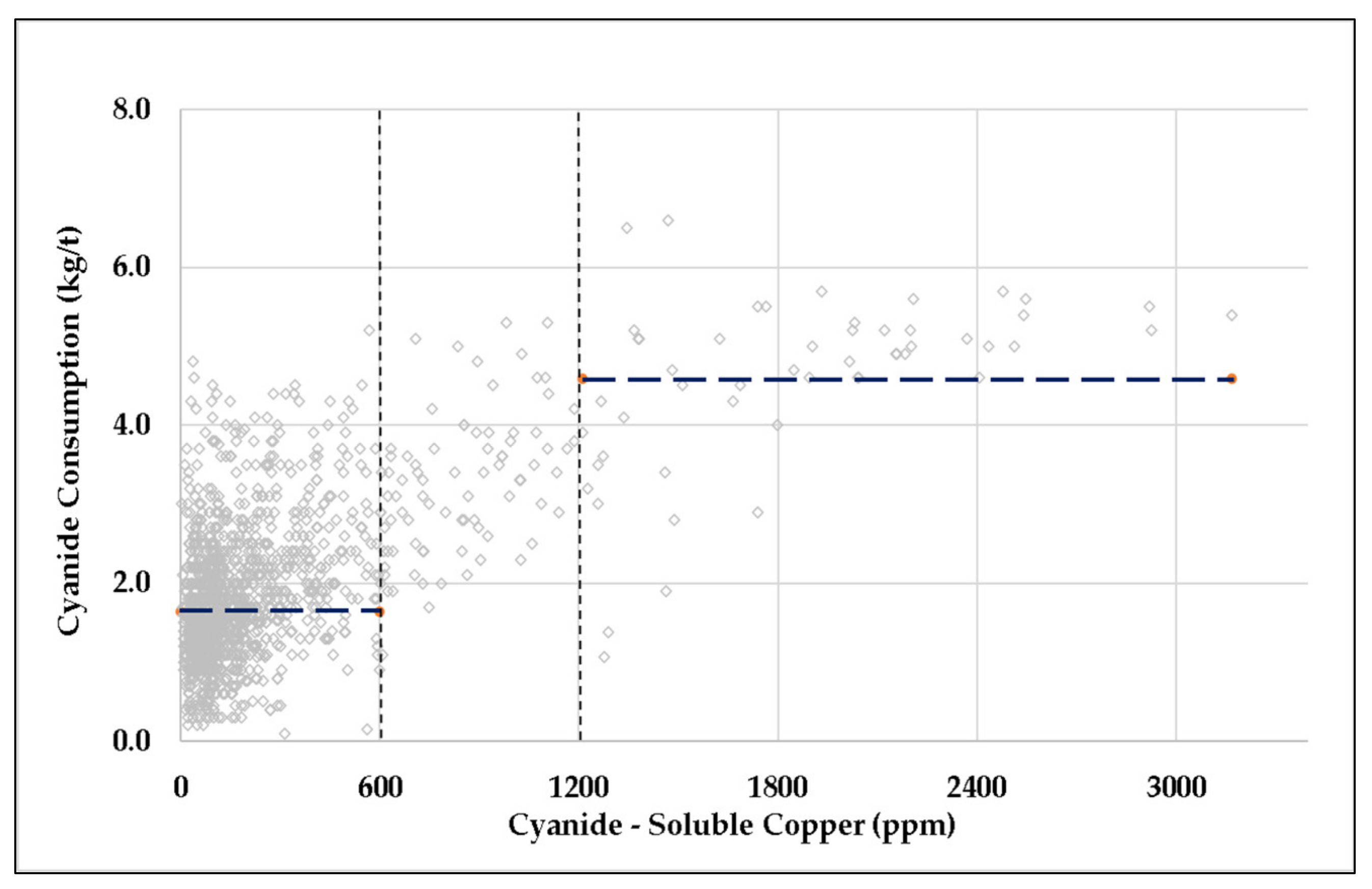
The DES/DRS framework of Navarra et al. [1] was successfully adapted to represent spikes in cyanide consumption at Minera Florida [2], considering the following threshold-crossing events:

• Stockout of HCC ore;
• Stockout of LCC ore;
• Reestablishment of target level for total stockpile (LCC + HCC);
• Transition to the next geological parcel.

As will be described in Section 3.2, stockouts trigger contingency processing modes. The notion of a “geological parcel” is described in [6] and provides a basic representation of geostatistical variation; each parcel contains a balance of HCC and LCC ore, which is the result of RNG. When detailed geospatial data (i.e., drill core samples) are available, the balance of HCC/LCC can be the result of a sequential Gaussian simulation [27], which is the subject of ongoing work [28]. For the current study, it is sufficient to consider:

• In the event that the parcel, k − 1, is completely excavated, a following parcel, k, is generated that will contain the next m_k tonnes of ore to be excavated;
• There is a 70% chance that parcel k is within the same facies as k − 1; if so, then the weight fraction of LCC in parcel k, denoted as $w_k^{\mathrm{LCC}}$, is generated according to a Gaussian distribution centered at $w_{k-1}^{\mathrm{LCC}}$, with the small standard deviation, σ_interfacies;
• Otherwise, if parcel k is in a new facies, then $w_k^{\mathrm{LCC}}$ is generated independently of the previous parcel, according to a Gaussian distribution centered on the orebody average and with a comparatively large standard deviation σ_orebody > σ_interfacies.

This basic representation considers only two ore classes (also known as geometallurgical units), such that the weight fraction of HCC is given by $w_k^{\mathrm{HCC}}=1-w_k^{\mathrm{LCC}}$. The DES/DRS framework can consider a higher number of ore classes, depending on the context, but these two classes have been sufficient to represent the Minera Florida context. Moreover, the mass m_k of parcel k is generated according to a uniform distribution; other distributions have been tested for this purpose, but they have no significant effect.

Arguably, a logical continuation of the work by Órdenes et al. [2] could include a detailed drill core sampling campaign to replace the parcel-based geological representation [6] and thus link the DRS system dynamics to ongoing efforts in geospatial orebody modelling [27,28]. However, prior to such a costly effort, numerous process variables should be explored and represented within the framework, including gold head grade. From a managerial point-of-view (Figure 2a), this detailing shows how the data which would result from such a campaign would contribute to continuous improvement efforts and upcoming plant upgrades. Indeed, the previous effort successfully captures the phenomenon of cyanide consumption within the simulation framework [2], yet the management at Minera Florida were surprised that only a small amount of the extensive data that they had provided had been utilized.

Following the approaches for the DES of manufacturing systems [18], the parameterization of process-variable distributions is an extension of standard exploratory data analysis (EDA). Depending on the context, standard EDA usually includes a listing of descriptive statistics such as mean, standard deviation, extreme observations (maxima and minima), and quartile data, as well as histograms and possibly other graphical constructions [29]. The quartile data are often used to establish criteria for outlier filtering. Figure 4 illustrates the use of maximum likelihood estimation (MLE) and goodness-of-fit statistics (GOF) in order to enhance a DES/DRS model; this type of detailing can be situated within the improvement cycle of Figure 2 if we consider that a data-driven probability distribution of a process variable is itself a submodel that replaces the deterministic representation.

The conversations that followed the first collaboration with Minera Florida [2] have emphasized the practical relevance of the data-driven parametrization of probabilistic distributions within gold extractive metallurgy (and ostensibly in other areas of mining and metallurgy). Without developing a convincing connection to the available plant data, the simulations may be rightly criticized for lacking a connection to production metrics, even if the most critical phenomena are well represented. Yet there seems to be an underrepresentation of journal articles detailing the contextualized application of MLE and GOF techniques within extractive metallurgical simulations. With the exception of the current work, we have failed to find such a paper.

3. Data-Driven Simulation of the Minera Florida Cyanidation Process

3.1. Exploratory Data Analysis and Fitting of Gold Head Grade Distributions

Based on its current mineral processes flow sheet, Minera Florida had previously run a detailed geometallurgical characterization program to link vein mineralogy to the metallurgical behavior of the ore fed into the cyanidation process. This sampling campaign included 1214 ore samples from different workfaces, classified in situ and tested at the on-site metallurgical laboratory. The samples were analyzed by a shaker test to determine a range of process parameters and related cyanide consumption (

Table 1. Summary of shaker test analytical conditions.

Parameters	Quantity
Ore Mass (g)	30
Granulometry (µm)	100%–200#
Solution Volume (mL)	60.00
Solid Percentage (%)	33.00
NaCN Concentration (g/L)	10.00
Pulp pH	11.00
Head Grade Assay	Au, Ag, Cu, *Fe
Leached Solution Assay	Cu, Fe, Free CN, *Au, *Ag
Tail Grade Assay	*Au, *Ag

).

From the information collected during the sampling campaign and the analytical results from the tested samples, a new geometallurgical ore classification was defined. This new ore classification is (1) in alignment with the four geological domains presented by Órdenes et al. [2], namely the oxide, mixed, low-Cu sulfide, and high-Cu sulfide domains, and (2) are further grouped by a combination of metallurgical behavior, field observed copper, and iron mineralogy, coupled with interpreted redox states and process impurities, including CuS and FeS, all of which relate to sodium cyanide consumption [2,11]. The presence of processed impurities (such as copper, iron, and sulfur) within the different orebodies exploited by Minera Florida, has a high potential of generating undesired reactions including the formation of thiocyanate and the dissolution of the transition metals, Cu, Fe, and Zn. Consequently, this new mineralogical scenario can inflict extra operational costs and diminished profits resulting from high levels of cyanide consumption [11,30].

Following on from the understanding gained at Minera Florida and from previously published work [2], the head grades from the tested samples have been separated into two geometallurgical units; these are high-cyanide-consuming (HCC) sulfides and low-cyanide-consuming (LCC) sulfides. This is an enhancement over the previously published work, which, although did consider the two units, did not consider the head grade distribution data. The basic descriptive statistics for the HCC and LCC geometallurgical units are given in

Table 2. Cyanide consumption per geometallurgical unit.

Variable	Statistics	High CN Consuming Sulfides	Low CN Consuming Sulfides
Cyanide soluble copper (ppm)	N° Samples	739	308
	Mean	310.26	176.22
	Standard Deviation	456.80	218.73
	Minimum	6.50	8.20
	Q1	80.60	65.05
	Q2	160.50	105.25
	Q3	319.65	204.53
	Maximum	3169.50	2480.20
Cyanide consumption (kg/t)	N° Samples	739	308
	Mean	2.24	1.75
	Standard Deviation	1.21	0.90
	Minimum	0.31	0.20
	Q1	1.40	1.10
	Q2	1.90	1.60
	Q3	2.80	2.20
	Maximum	7.40	5.70

as part of the initial exploratory data analysis (EDA). The samples describe the ore that is forecast over the medium term, originating from sampling campaigns that were extended from production tunnels.

The EDA was then extended to incorporate the gold head grade. A critical aspect of data analytics is handling anomalous data adequately [29]; this takes particular relevance when commodities grades are assessed, especially in gold [31]. Geostatisticians have proposed and used different techniques to mitigate the impact of high-grade data on mineral resource estimation; hence, the same procedures can be utilized in simulations to manage head grades. Various methods generally involve some form of capping and/or high-grade influence restrictions to mitigate the disproportionate influence of true outlier values on the contained metal within a resource. High values may arise because of sampling errors or reflect distinct geological sub-environments or domains within a mineral deposit [32]. Efforts must be directed to examining these high values and their geological context to distinguish errors from “real” high grades, investigating their characteristics and how they relate to the mineral inventory estimates [32]. In calculating the descriptive statistics for gold head grade, a data-cleansing procedure was applied to the Minera Florida data, given by:

$$Lower limit=Q1-1.5\cdot \left(Q3-Q1\right)$$

(20)

$$Upper limit=Q3+1.5\cdot \left(Q3-Q1\right)$$

(21)

These criteria have resulted in the elimination of 49 outliers from high cyanide consuming (HCC) Sulfides and 24 outliers from low cyanide consuming (LCC) sulfides, entirely from the upper limit in both cases.

A summary of the preprocessed statistics for gold head grade from the geometallurgical sample set is summarized in

Table 3. Gold head grade statistics by geometallurgical unit.

Variable	Statistics	High CN Consuming Sulfides	Low CN Consuming Sulfides
Gold Head Grade (g/t)	N° Samples	673	278
	Mean	5.07	3.56
	Standard Deviation	2.92	1.88
	Kurtosis	0.29	0.46
	Skewness	0.99	1.00
	Minimum	0.24	0.18
	Q1	2.81	2.11
	Q2	4.29	3.22
	Q3	6.61	4.55
	Maximum	14.39	9.04

. The data in this table, and throughout the remainder of the paper, were computed subsequent to the aforementioned elimination of outliers (Equation (21)).

Gold grades from vein-style gold deposits are highly variable and are often complex and erratic, but commonly show skewed positive grade distribution [19]. Their complexity is typically reflected in two components: (1) low-grade continuity and (2) diversity of ore trends. Gold grades are commonly related to variably-sized ore shoots of high-grade mineralization surrounded by lower-graded areas; yet, ore shoots may account for a relatively small proportion of the total mineralization [19]. For the Minera Florida dataset, the histogram of gold grades for both geometallurgical units shows a positive skewness (Sk >0.5, Table 3) and low kurtosis (Table 3), and a platykurtic shape (Figure 8). The histograms for both geometallurgical units show high variability and high-grade tail.

Table 4. Ranking of distributions in accordance with GOF metrics.

High Cyanide Consuming Sulfides
	Chi-Square		Kolmogorov-Smirnov		Anderson-Darling
Distribution	Statistics	Rank	Statistics	Rank	Statistics	Rank
Pearson 5	8.15	1	0.050	22	4.04	25
Fatigue Life	12.09	2	0.030	3	1.46	2
Log-Normal	12.41	3	0.032	4	1.41	1
Pearson 5 (3P)	14.19	4	0.059	28	9.84	33
Dagum	14.94	5	0.040	8	2.54	10
Dagum (4P)	18.17	6	0.043	14	2.56	11
Log-Logistic (3P)	19.14	7	0.042	9	2.71	12
Log-Logistic	19.77	8	0.048	18	3.06	14
Fatigue Life (3P)	20.86	9	0.040	7	1.97	4
Log-Normal (3P)	22.22	10	0.039	6	2.09	5
Gaussian	170.21	42	0.116	40	18.89	38
Low Cyanide Consuming Sulfides
	Chi-Square		Kolmogorov-Smirnov		Anderson-Darling
Distribution	Statistics	Rank	Statistics	Rank	Statistics	Rank
Pearson 5 (3P)	7.64	1	0.053	18	3.67	30
Inv. Gaussian	7.93	2	0.044	9	0.98	11
Fatigue Life	9.40	3	0.065	25	1.32	17
Frechet	10.52	4	0.080	30	4.65	34
Pearson 5	11.23	5	0.070	26	3.12	29
Log-Normal	11.80	6	0.044	8	0.62	1
Gamma	17.24	7	0.055	19	1.28	16
Gen. Extreme Value	17.37	8	0.041	1	0.83	2
Log-Logistic	17.44	9	0.045	10	0.84	3
Dagum	18.27	10	0.043	6	0.89	5
Gaussian	70.27	42	0.125	39	7.10	36

lists the candidate distributions in terms of their goodness-of-fit metrics for several candidate distributions, indicating that the log-normal was an acceptable choice for representing the gold head grades; it ranked highly in χ² and KS as third and fourth, respectively, and was the top-ranked distribution in both cases for AD. These results were obtained using the easy fit software developed by Math Wave Technologies. Looking at the HCC data, a consideration may be given to the Pearson 5 distribution, after having ranked well in terms of χ² but with a low ranking in KS and AD. Perhaps a better case can be made for the fatigue life distribution (also known as Birnbaum–Saunders distribution), which surpassed the log-normal for χ² and KS for HCC, although it did not perform especially well in KS and AD for LCC and is a somewhat obscure; to be fair, the fatigue life distribution represents model equipment failure times, with a flash occurrence of cyanide-consuming minerals being likened (debatably) to a spontaneous equipment breakdown. Nonetheless, the case for log-normal is clearly the strongest candidate for HCC. Although the inverse Gaussian and general extreme value distributions could be considered for LCC, these distributions are comparatively difficult to use for this purpose since they are not commonly used, and the more common log-normal was the highest ranked in AD. For general interest, the poorly ranked Gaussian distribution is included in Table 4.

The choice of the log-normal is further corroborated by the χ² and Kolmogorov–Smirnov GOF hypothesis tests, as summarized in

Table 5. Summary of goodness of fit tests for the log-normal, α = 0.05.

High CN-Consuming Sulfides	Critical Value	Observed Value	Null Hypothesis
Chi-Squared (Degrees of Freedom = 8)	15.51	12.41	H0 is accepted for Log-Normal Distribution
Kolmogorov—Smirnov	0.034	0.031	H0 is accepted for Log-Normal Distribution
Anderson-Darling	0.87	1.40	H0 is rejected for Log-Normal Distribution
Low CN-Consuming Sulfides	Critical Value	Observed Value	Null Hypothesis
Chi-Squared (Degrees of Freedom = 7)	14.07	11.80	H0 is accepted for Log-Normal Distribution
Kolmogorov—Smirnov	0.053	0.045	H0 is accepted for Log-Normal Distribution
Anderson-Darling	0.87	0.61	H0 is accepted for Log-Normal Distribution

. However, in the case of the HCC geometallurgical unit, the null hypothesis (that the data are characterized by log-normal) is rejected according to the Anderson–Darling (AD) test, at 95% significance, but is nonetheless accepted by the χ² and Kolmogorov–Smirnov tests. As noted in Section 2.2, the AD emphasizes (and possibly over-penalizes) the extreme values; even after the preprocessing described by Equations (20) and (21), the HCC data include unusually high grades, exceeding 13 g/t, but this corresponds to only 1.2% of the samples. However, the rejection of the top-ranked AD distribution (Table 4) when subjected to the AD hypothesis (Table 5) is moot since the actual head grades that will be received by the Florida plant will follow a distribution that is more complex than the log-normal and any other commonly available distribution, with this dependent on both the geospatial distribution of the minerals as well as the excavation sequence. This will be further discussed in Section 4. Interestingly, the log-normal is accepted in the case LCC for all three GOF tests.

The GOF computations of Table 4 and Table 5 considered the MLE parametrization of the solutions, computing this from the cleansed data described in Table 3. Considering that the log-normal distribution was selected for geometallurgical units, the corresponding parameter values are given in

Table 6. Maximum likelihood estimation results.

Maximum Likelihood Estimation (MLE)	Gold Head Grade Estimator HCC	Gold Head Grade Estimator LCC
$\widehat{\mathit{\mu }}$	4.29	3.09
$\widehat{\mathit{\sigma }}$2	1.42	1.35

. These results were provided by easy fit and were verified by Equations (6) and (7) prior to being programmed into the discrete rate simulations that will now be described.

3.2. Discrete Rate Simulation of the Minera Florida Cyanidation Process

The previous result presented by Órdenes et al. [2] featured the classification of ore into two geometallurgical ore types (high- and low-cyanide-consuming ores) that are managed by alternating between modes of operation. The alternating modes provide an integrated response to changes in the feed mineralogy and other operational conditions within the mineral value chain. Processing plants are generally designed to maximize profits while respecting technological limitations, environmental norms, and tactical constraints that align operational objectives with long-term strategic goals. For an underground mine, the variation in stockpile levels is typically intensified due to a variety of factors, including (1) a large number of concurrent active workfaces (ore type variability); (2) ore grade-driven mine planning that does not consider geometallurgical inputs; and (3) the uncertainty caused by complex extraction methods, which rely on the coordination of many variables (e.g., ventilation, drainage, equipment availability) to meet planned production [2]. All of these factors add to the variability in the feeds being received by the Minera Florida cyanidation plant district, which has motivated the adaptation of a DES/DRS to improve decision-making and evaluate the effects of the stockpile management in the plant performance. The critical aspect of balancing the two geometallurgical units was addressed in the previous work [2] and is now extended to incorporate gold head grades.

To achieve the best performance of the mining system under study, alternating configurations and modes are represented within the current framework to help maintain consistency in ore feeding. The selection of a configuration depends on the forecasted timing of stockouts in HCC and LCC, given their requirement for feed blending. In the case of Alhué ore, the operational policies were designed to maximize tonnage and stabilize cyanide consumption within the regular mode of configuration A (

Table 7. Description of operational modes in relation to possible deposit forecast, including gold head grades.

	Deposit	Configuration A		Configuration B
Parameters	Average	Regular	Contingency	Regular	Contingency
HCC-Ore 1 in feed (%)	60	55	100	70	0
LCC-Ore 2 in feed (%)	40	45	0	30	100
Gold Head Grade (g/t)	3.81	3.75	4.29	3.93	3.09
Throughput (kt Ore/day)	-	2.7	2.3	2.4	1.2
Cyanide Consumption (kg/t)	-	2.02	2.24	2.09	1.75

). This mode (called “A-regular”) brings the plant to its maximum productive capacity while minimizing cyanide consumption. Nonetheless, if at the end of a production campaign, the LCC stockpile is below a predetermined threshold, the plant is then reconfigured into configuration B, whose regular mode (called “B-regular”) is designed to rebuild the LCC stockpile while still avoiding the risks of spikes in cyanide consumption. If a stockout occurs during a production campaign, a contingency mode is applied, in which only the available type of ore is consumed to allow the depleted ore type to accumulate again before returning to the regular configuration. Thus, the mode changes from A-regular to A-contingency if there is an LCC stockout during a campaign of configuration A; similarly, the mode changes from B-regular to B-contingency if there is an HCC stockout during a campaign of configuration B.

For the current set of simulations, A-contingency consumes only HCC ore, which allows the LCC stockpile to rebuild as quickly as possible, while B-contingency consumes only LCC ore, allowing the HCC stockpile to rebuild (Table 7). Because contingency modes are less productive than the regular modes, the duration of contingency segments has been set to one day, causing the plant to alternate between regular and contingency until the next planned shutdown. In reality, the contingency durations can be longer than a day, depending on how much longer is remaining in the current production campaign (Some discussions have been made regarding how to better represent the contingency durations to capture the actual operational decisions that are taken, but an improved submodel has yet to be developed in this regard).

The values posted in Table 7 regarding Configuration A are based on reconciled mass balances from data from Minera Florida between June 2020 to February 2021. Considering that HCC has a grade of 4.29 g/t and LCC of 3.09 g/t and has a 55-45 blending that gives a 3.75 g/t regular head grade, the throughput and cyanide consumption also correspond to this same time period. On the other hand, the data from Configuration B are hypothesized to accommodate more HCC ore but at the expense of throughput rather than spiking cyanide consumption; the same HCC and LCC grades as those within Configuration A are maintained for quantifying Configuration B, but with a different blend (70-30). Conceptually, a combination of the A-regular and B-regular modes allows the plant to adapt to the deposit average. In general, if a new configuration is being developed such that it can be initially parametrized by laboratory results and/or by early plant tries, but ultimately, after it has been implemented, the accumulated plant data must be used to verify the performance.

The decision to alternate between modes depends on current and forecasted stockpile levels [2]. This research follows the approach proposed by Navarra et al. [1], wherein two operational policy parameters, also known as control variables, characterize the decision-making: X = Target Ore Stockpile Level and Y = LCC Critical Stockpile Level. To coincide with the formulation of [1], the high-cyanide-consuming ore is considered to be Ore 1 whereas the low-cyanide-consuming ore is Ore 2; thus, when the stockpile of LCC falls below the user-specified Y value, the decision is made to convert the system into configuration B at the following shutdown. The simulated gold head grades and the average of the gold ounces fed into the plant are presented in Figure 8. These consider the variation of the stockpile levels of the two sulfide geometallurgical units of the Alhué district (Figure 9).

The analysis of the dynamics of the mining system, based on the inventory management strategies and modes of operation, shows that an orebody average of 3.81 g/t is attainable (considering 60% HCC ore and 40% LCC ore, Table 7). The highest production of ounces of gold is obtained when the total target inventory level is set to 10,000 tons, and the critical LCC stockpile level is set to 1000 tons, where the maximum production is 315.39 oz/day. This outcome is due to the greater availability of ore and to a less constrained system due to decreased occurrences of LCC shortages. Conversely, the configuration that minimizes the available stock (X = 6000 t and Y = 4000 t), with a head grade result of 3.72 g/t (one of the lowest head grade results,

Table 8. Summary of discrete event simulation throughputs, cyanide consumption, and simulated gold grades.

Target Stockpile Level	Critical Ore Stockpile Level	1000 t	2000 t	3000 t	4000 t
6000 t	Mean Average Throughput (t)	2549.51	2541.28	2525.46	2503.90
	Mean Average CN Consumption (kg/t)	2.044	2.042	2.040	2.038
	Max Average Gold Head Grades (g/t)	4.03	3.96	4.02	4.00
	Mean Average Gold Head Grades (g/t)	3.73	3.72	3.72	3.72
	Min Average Gold Head Grades (g/t)	3.40	3.44	3.43	3.42
	Max Average Gold in metal (oz/day)	333.88	327.35	328.27	325.86
	Mean Average Gold in metal (oz/day)	305.69	304.24	301.34	299.54
	Min Average Gold in metal (oz/day)	276.37	278.81	275.16	272.37
8000 t	Mean Average Throughput (t)	2581.31	2579.32	2572.19	2554.89
	Mean Average CN Consumption (kg/t)	2.047	2.046	2.045	2.045
	Max Average Gold Head Grades (g/t)	4.00	4.02	3.98	4.00
	Mean Average Gold Head Grades (g/t)	3.76	3.75	3.74	3.74
	Min Average Gold Head Grades (g/t)	3.41	3.43	3.47	3.46
	Max Average Gold in metal (oz/day)	334.60	336.12	332.48	331.50
	Mean Average Gold in metal (oz/day)	312.11	310.81	309.63	307.10
	Min Average Gold in metal (oz/day)	281.19	282.80	284.60	280.67
10,000 t	Mean Average Throughput (t)	2592.84	2594.79	2592.99	2588.51
	Mean Average CN Consumption (kg/t)	2.047	2.046	2.045	2.045
	Max Average Gold Head Grades (g/t)	4.01	4.03	4.02	4.02
	Mean Average Gold Head Grades (g/t)	3.78	3.78	3.77	3.76
	Min Average Gold Head Grades (g/t)	3.41	3.46	3.39	3.41
	Max Average Gold in metal (oz/day)	336.56	337.82	337.25	336.64
	Mean Average Gold in metal (oz/day)	315.39	315.35	314.29	312.80
	Min Average Gold in metal (oz/day)	282.40	286.57	281.37	282.47

) and throughput result of 2503.90 t (the lowest tonnage result), is a system configuration that produces the second lowest value of the average ounces: 299.54 oz/day. In this case, the system is constrained due to the continuous LCC ore shortages under configuration A and HCC shortages under configuration B, causing decreases in throughput and lower recovery.

By verifying the results, it is possible to establish that the optimal configuration for the control variables for the modelled mining system is X = Target Ore Stockpile Level = 10,000 t, and Y = LCC Critical Stockpile Level = 2000 t. These dynamics reach the best performance, achieving the highest throughput (2594.79 t, Table 8) and the second-best result in fed ounces (315.35 oz/day, Table 8). Under this system configuration, the key performance indicators (KPI) are maximized, as throughput and gold head grades reach values that are close to those predicted by the orebody average. Additionally, a stable sodium cyanide dosage is attained, despite the process being subject to heterogeneous feeds [2].

Moreover, additional benefits from an appropriate set of the target ore stockpile level allow for longer operational plant stability timeframes, supported by more extended periods in configuration A (with time in configuration A > configuration B, Figure 10a) in comparison with a lower Target Ore Stockpile Level (Figure 10a). In this context, minimizing this control variable is an operational decision that mine managers must face while considering the effects of this on the KPIs. For instance, having a low ore stockpile level available means that the system is at risk of suffering constant ore-shortage events.

Another adverse effect generated by low mineral stockpiles is the continuous changes of modes of operation within a production campaign, from A-regular to A-contingency and B to B-contingency in cyclic time intervals, caused by the frequent stockouts of ore 2, which occur under mode A-regular and stockouts of ore 1 under mode B-regular (Figure 11). This is what can adversely affect mill productivity, which is seen as the tight sawtooth shapes, more frequent in Figure 11a than in Figure 11b, albeit in shorter spurts. On rare occasions, there can be an unlikely stockout of ore 1 under A-regular, which is shown in Figure 11a starting at day 580, as the excavation zones are unexpectedly low in ore 1; similarly, there can be an unlikely stockout of ore 2 under B-regular (which is not shown in Figure 11 but has been observed in other simulations). For these unlikely stockouts, the operations are programmed to temporarily increase the mining rate (i.e., perform a “mining surge”), which assures that the plant receives the regular feed blend. As observed in Figure 11a at day 580, the assurance of ore 1 requires the simultaneous excavation of excessive ore 2, and the target ore stockpile level cannot be reestablished until roughly day 590. Nonetheless, these mining surges do not affect the overall throughput as the mill continues to receive the regular feed; rather, it is the alternation of contingency modes (tight sawtooths) that correspond to lost production.

The optimal configuration of 10,000 t target ore stockpile level and 2000 t LCC critical stockpile level, in which the ore shortage events are more likely (Figure 11b), is compared with other stockpile levels with lower target ore stockpile levels. As a result, the system occasionally enters the less productive contingency modes. This can be estimated as a 5% loss of benefit in daily ounces production, comparing the best result with the 6000 t target ore stockpile level and 4000 t LCC critical stockpile level configuration.

4. Conclusions and Future Work

The main objective of this work was (1) to demonstrate the data-driven incorporation of gold head grades into the DES/DRS framework that was developed to represent the operations at Minera Florida and (2) to visualize the dynamics in the system of the new variable under study. This research also confirms that the critical variable, target ore stockpile level, is crucial for maximizing gold head grade and tonnage, and indeed, metal production. This same approach is being used to represent other process variables for the simulation of Minera Florida processes in addition to gold head grade. The incorporation of this into the DRS framework of key performance indicators (KPIs), in conjunction with gold head grade and other process variables, helps managers to improve the decision-making process under successive detailing from system simulations (Figure 2). In the same direction, with a better understanding of the dynamics of the different parameters within each system, it is possible to identify potential risks that may affect these critical variables, so far as at the strategic level (long-term planning) and at the tactical level (short-term planning).

The future line of this research is to incorporate variables that have a high potential to impact economic profitability, for example, energy consumption. The advantage of simulation using different variables is that this technique can be used to explore a number of system scenarios, allowing users to visualize those risks that have multidisciplinary aspects, such as evaluating the sustainability of mining projects. Understanding the system’s dynamics can help to improve the handling of harmful contaminants, optimize mineral process reagents (e.g., cyanide consumption as studied in this sequence of works), improve processed water management, and decrease the carbon dioxide footprint (optimization of energy consumption).

Finally, a complement to this research, in discrete rate simulation frameworks (Figure 2), is the parallel development of programmed routines that allow the simulation platform to draw geological attributes directly from block models and mine plans. This points toward experimentation with the incorporation of geostatistical techniques (e.g., stochastic ore body modelling, sequential Gaussian simulations, Kriging estimation, etc.) that allow the linking of feed variability with the geospatial aspects of the orebody and the mine plan.

References

1. Navarra, A.; Alvarez, M.; Rojas, K.; Menzies, A.; Pax, R.; Waters, K. Concentrator operational modes in response to geological variation. Miner. Eng. 2019, 134, 356–364. [Google Scholar] [CrossRef]
2. Órdenes, J.; Wilson, R.; Peña-Graf, F.; Navarra, A. Incorporation of Geometallurgical Input into Gold Mining SystemSimulation to Control Cyanide Consumption. Minerals 2021, 11, 1023. [Google Scholar] [CrossRef]
3. Boom, R.; Twigge-Molecey, C.; Wheeler, F.; Young, J. Metallurgical Plant Design; Canadian Institute of Mining, Metallurgy and Petroleum: Montreal, QC, Canada, 2015. [Google Scholar]
4. Mittal, S.; Zeigler, B.P.; Martin, J.L.R.; Sahin, F.; Jamshidi, M. Modeling and Simulation for Systems of Systems Engineering. In System of Systems Engineering: Innovations for the 21st Century; Wiley: Hoboken, NJ, USA, 2008; Chapter 5; pp. 101–149. [Google Scholar]
5. Wilson, R.; Mercier, P.H.J.; Navarra, A. Integrated Artificial Neural Network and Discrete Event Simulation Framework for Regional Development of Refractory Gold Systems. Mining 2022, 2, 123–154. [Google Scholar] [CrossRef]
6. Peña-Graf, F.; Órdenes, J.; Wilson, R.; Navarra, A. Discrete Event Simulation for Machine-Learning Enabled Mine Production Control with Application to Gold Processing. Metals 2022, 12, 225. [Google Scholar] [CrossRef]
7. Peña-Graf, F.A.; Grammatikopoulos, T.; Kabemba, A.; Navarra, A. Integrated feed management of mineral processing plants with application to chromite processing. Can. Metall. Q. 2021, 60, 130–136. [Google Scholar] [CrossRef]
8. Wilson, R.; Perez, K.; Toro, N.; Parra, R.; Mackey, P.J.; Navarra, A. Mine-to-smelter integration framework for regional development of porphyry copper deposits within the Chilean context. Can. Metall. Q. 2022, 61, 48–62. [Google Scholar] [CrossRef]
9. Sadehi, M.; Houdouin, D.; Bazin, C. Mineral processing plant data reconciliation including mineral mass balance constraints. Miner. Eng. 2018, 123, 117–127. [Google Scholar] [CrossRef]
10. Han, S.; Jung, M.; Lee, W.; Kim, S.; Lee, K.; Lim, G.-t.; Jeon, H.-S.; Choi, S.Q.; Han, Y. Diagnosis and Optimization of Gold Ore Flotation Circuit via Linear Circuit Analysis and Mass Balance Simulation. Minerals 2021, 11, 1065. [Google Scholar] [CrossRef]
11. Hedley, N.; Tabachnick, H. Chemistry of Cyanidation; Mineral Dressing Notes No. 23; American Cyanamid Company: New York, NY, USA, 1958. [Google Scholar]
12. Guo, B.; Peng, Y.; Espinosa-Gomez, R. Cyanide chemistry and its effect on mineral flotation. Miner. Eng. 2014, 66–68, 25–32. [Google Scholar] [CrossRef]
13. Camus, F.; Boric, R.; Skewes, M.A.; Castelli, J.C.; Reichhard, E.; Mestre, A. Geologic, Structural, and Fluid Inclusión Studies of El Bronce Epitermal Vein System, Petorca, Central Chile. Econ. Geol. 1991, 86, 1317–1345. [Google Scholar] [CrossRef]
14. Diaz, S. Geología Económica y Prospección Geoquímica del área de la Mina La Leona, Distrito Minero Chancón, VI Región; Memoria Para Optar al Título de Geólogo; Universidad de Chile: Santiago, Chile, 1986; 196p. [Google Scholar]
15. Morris, H.T.; Fisher, F.S.; Shawe, D.R.; Thompson, T.B. Gold-Bearing Polymetallic Veins and Replacement Deposits Part II. In Geology and Resources of Gold in the United States; Bulletin 1857-F; U.S. Geological Survey: Reston, VA, USA, 1990. [Google Scholar]
16. Xue, G.; Zhang, L.; Hou, D.; Liu, H.; Ding, Y.; Wang, C.; Luo, X. Integrated geological and geophysical investigations for the discovery of deeply buried gold–polymetallic deposits in China. Geol. J. 2019, 55, 1771–1780. [Google Scholar] [CrossRef]
17. Devore, J.L. Inferences Based on Two Samples. In Probability and Statistics for Engineering and the Sciences, 8th ed.; Cengage Learning: Boston, MA, USA, 2011; Chapter 9; pp. 345–390. [Google Scholar]
18. Altiok, T.; Melamed, B. Simulation Modeling and Analysis with Arena; Academic Press: San Diego, CA, USA, 2007. [Google Scholar]
19. Dominy, S.C.; Stephenson, P.R.; Annels, A.E. Classification and reporting of mineral resources for high-nugget effect gold vein deposits. Explor. Min. Geol. 2001, 10, 215–233. [Google Scholar] [CrossRef]
20. Ferguson, K.D.; Erickson, P.M. Pre-Mine Prediction of Acid Mine Drainage. In Environmental Management of Solid Waste; Salomons, W., Förstner, U., Eds.; Springer: Berlin/Heidelberg, Germany, 1988; pp. 24–41. [Google Scholar] [CrossRef]
21. Montgomery, D.C.; Runger, G.C. Sampling Distributions and Point Estimation of Parameters. In Applied Statistics and Probabilty for Engineers, 5th ed.; John Wiley & Sons: Hoboken, NJ, USA, 2010; Chapter 7; pp. 223–250. [Google Scholar]
22. Devore, J.L. The Chi-Squared Distribution. In Probability and Statistics for Engineering and the Sciences, 8th ed.; Cengage Learning: Boston, MA, USA, 2011; Chapter 4; pp. 137–192. [Google Scholar]
23. Massey, F.J., Jr. The Kolmogorov-Smirnov Test for Goodness of Fit. J. Am. Stat. Assoc. 1951, 46, 68–78. [Google Scholar] [CrossRef]
24. Anderson, T.W.; Darling, D.A. A test of goodness of fit. J. Am. Stat. Assoc. 1954, 49, 765–769. [Google Scholar] [CrossRef]
25. Devore, J. The Analysis of Variance. In Probability and Statistics for Engineering and the Sciences, 8th ed.; Cengage Learning: Boston, MA, USA, 2011; Chapter 10; pp. 391–418. [Google Scholar]
26. Pearson, K. On the criterion that a given system of deviations from the probable in the case of a correlated system of variables is such that it can be reasonably supposed to have arisen from random sampling. London Edinb. Dublin Philos. Mag. J. Sci. 1900, 50, 157–175. [Google Scholar] [CrossRef]
27. Bai, T.; Tahmasebi, P. Sequential Gaussian simulation for geosystems modeling: A machine learning approach. Geosci. Front. 2021, 13, 101258. [Google Scholar] [CrossRef]
28. Órdenes, J. Discrete Rate Simulation Throughput Optimization of High-grade Ag-Ag Low Sulphidation Vein Hosted Deposits based on Sequential Gaussian Simulation of Cyanide Consumption. In Proceedings of the 21st Annual Conference of thr International Association for Mathematical Geosciences, Nancy, France, 29 August–3 September 2022. [Google Scholar]
29. Komorowski, M.; Marshall, D.C.; Salciccioli, J.D.; Crutain, Y. Exploratory Data Analysis. In Secondary Analysis of Electronic Health Records; MIT Critical Data, Ed.; Springer Nature: Berlin/Heidelberg, Germany, 2016; Chapter 15. [Google Scholar]
30. Habashi, F. Kinetics and Mechanism of Gold and Silver Dissolution in Cyanide Solution; Montana Bureau of Mines and Geology Bulletin 59; Montana Bureau of Mines and Geology: Butte, MT, USA, 1967. [Google Scholar]
31. Filiben, J.J.; Heckert, A. Exploratory Data Analysis. In NIST/SEMATECH e-Handbook of Statistical Methods; NIST/SEMATECH: Gaithersburg, MD, USA, 6 July 2003. [Google Scholar]
32. Kehmeier, R.; Acuña, E.; Hartman, B.; Zeise, J. Management of Extreme High Grade Assay in Mineral Resource Estimates. RPM Global, 2016. Available online: www.rpmglobal.com (accessed on 17 August 2022).
Figure 1. Summative data from Minera Florida from June 2020 to February 2021 regarding the processing of ores from the Alhué district, demonstrating that spikes in cyanide consumption (expressed in kg of cyanide per tonne of feed) are associated with higher quantities of cyanide-soluble copper, carried by the feed. “Cyanide-soluble copper” includes copper from chalcocite/digenite, covellite, and bornite, but not chalcopyrite and tetrahedrite/tennatite.
Metals 12 01372 g001
Figure 2. Development of extensible simulation framework prior to approval of metallurgical studies: (a) interaction with management leading to approval; (b) detailing of simulation framework through the incorporation of models and submodels.
Metals 12 01372 g002
Figure 3. Maximum likelihood estimation is incorporated into common goodness-of-fit statistics, including χ2, Kolmogorov–Smirnov, and Anderson–Darling.
Metals 12 01372 g003
Figure 4. Data-driven representation of process variable distributions within a DES/DRS framework, using maximum likelihood estimation and goodness-of-fit ranking.
Metals 12 01372 g004
Figure 5. Kolmogorov–Smirnov statistic (KS) is the supremal distance between an empirical cumulative distribution and an MLE-parametrized cumulative distribution. A small KS indicates a good fit.
Metals 12 01372 g005
Figure 6. General representation of a Monte Carlo simulation framework.
Metals 12 01372 g006
Figure 7. Relationship between Monte Carlo, discrete event, and discrete rate simulation.
Metals 12 01372 g007
Figure 8. Gold head grade histograms for (a) the HCC geometallurgical unit and (b) the LCC geometallurgical unit.
Metals 12 01372 g008
Figure 9. Main simulation statistics as a function of policy parameter target stockpile levels, X = 10,000 t (Yellow line), 8000 t (Blue line), 6000 t (Red line), considering LCC critical stockpile levels, Y = 1000 t, 2000 t, 3000 t. (a) Gold head grade averages under different Target Ore Stockpile Levels. (b) Gold ounce averages fed into plant under different Target Ore Stockpile Levels.
Metals 12 01372 g009
Figure 10. Time distribution of operational modes in response to geometallurgical units with CN consumption variability for (a) target ore stockpile level critical at 10,000 t and LCC threshold of 2000 t, and (b) an enhanced configuration using a critical value of 6000 t and a target total stockpile level of 4000 t.
Metals 12 01372 g010
Figure 11. (a) System entering into A-Contingency and B-Contingency modes in cyclic time intervals due to the repeating shortages of HCC and LCC ores affecting the operational stability of the plant and the final KPI results. (b) Stockpile evolution during simulations with control parameters set at 10,000 t for the Target Ore Stockpile Level (TOSL) and 2000 t for the Critical LCC Stockpile Level, which shows some stockpile shortages and long timeframes without stockouts.
Metals 12 01372 g011