Data-Driven Construction Method of Material Mechanical Behavior Model

Abstract

To obtain the mechanical behavior response of the material under loading, a data-driven construction method of material mechanical behavior model is proposed, which is universal for predicting the mechanical behavior of any material under different loads. Based on the framework of artificial intelligence and finite element simulation, the method uses Python script to drive an Abaqus loop calculation to obtain data sets and performs artificial intelligence training on data sets to realize model construction. In this paper, taking the quasi-static tension of 9310 steel as an example, a material mechanical behavior model is constructed, and the accuracy of the prediction model is verified based on the experimental data. The results show that the simulation results are in good agreement with the experimental data. The error between the simulation results and the experimental results is within 2%, indicating that the model constructed by this method can effectively predict the mechanical properties of materials.

1. Introduction

The mechanical properties of a material are the properties it behaves with under external loads, and there are noticeable differences with different loads. In practical engineering problems, only by fully understanding the mechanical properties of materials can the service environment of materials be reasonably formulated, thereby ensuring their safety and reliability during service.

Conducting experiments is the most direct and effective way to obtain the mechanical behavior of materials. Scholars have constructed material constitutive models [1,2,3] using experiments to describe the stress–strain response of materials, and then study the mechanical properties of materials. Xin, X. [4] conducted compression experiments on TB8 titanium alloy at room temperature, studied the flow stress behavior of TB8 by analyzing stress–strain curves of titanium alloy with different strain rates, and finally established a dynamic plastic mathematical model of TB8 material. Cheng, Y. [5] conducted a series of dynamic tensile tests on Q235 steel using MTS material testing machine, Instron high-speed material testing machine, and Hopkinson bar. Then, they obtained stress–strain curves of different strain rates, and further studied the dynamic mechanical properties of Q235 steel. Based on a comprehensive analysis of experimental data, Gardner, L. [6] developed a predictive expression of material behavior, which can express the entire stress–strain response of cold-formed steel. Kweon, H.D. [7] and Zhao, K. [8], using typical tensile experiments combined with the method of finite element analysis, obtained the true stress–strain curve of the entire strain range of the material to analyze the mechanical properties of the material. The above studies show that the constitutive equation representing the mechanical behavior of materials can be well fitted by using experimental data under different conditions. Still, the constitutive equation obtained by fitting needs to be modified for other loads and materials, which lacks generality and increases the experimental cost.

In recent years, there has been continuous improvement of numerical simulation computing power; artificial neural networks, machine learning, and other artificial intelligence technologies have developed rapidly; and related advanced algorithms have been applied to many disciplines. Artificial intelligence technology provides new ideas for the research on frontier directions and hot issues of materials [9,10,11,12,13]. Compared with the traditional regression statistical mathematical model, the model constructed by artificial neural network shows superiority in terms of prediction accuracy, computational efficiency, and scope of application [14,15]. Naser M Z [16] used artificial intelligence and machine learning to construct a temperature-dependent material model of structural steel to accurately predict the temperature-dependent thermal and mechanical properties of structural steel. Jang D P [17] proposed a constitutive model based on machine learning to predict the elastic–plastic behavior of J2 plastic material. Artificial neural network was used to replace the nonlinear stress integral in isotropic hardening and related flow criteria under the traditional theoretical constitutive model, which ensured the prediction accuracy and improved the calculation efficiency. Stoffel M [18,19] used artificial neural network to replace the viscoplastic constitutive equation in the finite element to represent the generalized force and displacement relationship, which improved the simulation accuracy. At the same time, they omitted the constitutive calculation iteration process in the traditional finite element method, which significantly reduced the simulation time. Sharath B N [20] has built an artificial neural network framework with three-variable load, speed, and distance as input and weight loss as output. The generalization ability of the neural network is verified with experimental values, indicating that the neural network has established sufficient consistency between the experimental results and the results. Nagaraja, S. [21] has constructed an artificial neural network model to accurately predict the tensile properties of composites, which provides a framework for the prediction of tensile strength properties of composites with different reinforcement compositions and heat treatment conditions. The above literature shows that the artificial neural network can scientifically and reasonably construct the mapping relationship between material characteristics and target quantities, laying the foundation for the application of artificial intelligence in the mechanical properties of materials [22,23,24].

From the current related research, using artificial neural network to predict the mechanical behavior of materials has great potential in terms of experimental cost and prediction accuracy. Given this, in order to build a universal prediction model of material mechanical behavior, a method is proposed to build a prediction model of material mechanical behavior based on the artificial neural network by generating data sets through numerical simulation. This paper only takes the quasi-static tensile of 9310 steel as an example to build a material mechanical behavior model and verify the accuracy of the model with experimental data. In fact, the mechanical behavior model of materials constructed by this method is not only applicable to the study of quasi-static tensile mechanical behavior, but also applicable to the study of mechanical behavior of other loads and materials.

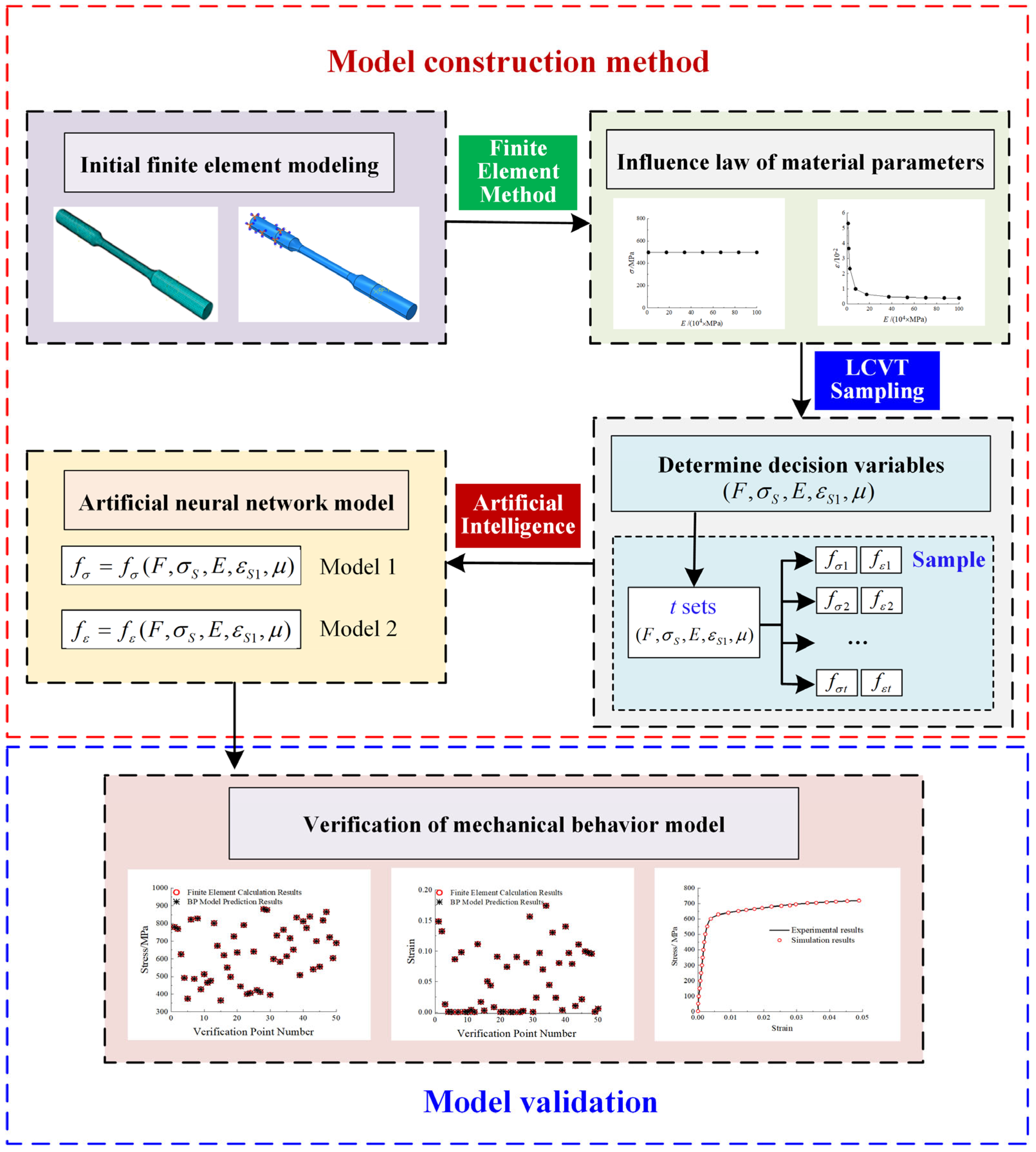
2. Ideas and Methods

The secondary development of Abaqus software is carried out based on the Python language, and the extracted decision variable combinations are sequentially substituted into the finite element numerical model for numerical solutions. A high-dimensional vector composed of each group of decision variables and their corresponding stress and strain is defined as a sample point. All sample points constitute a sample set, which provides data support for the construction of artificial neural network models. The model construction method is shown in Figure 1, and the key steps are as follows:

(1)

The initial finite element model is established;

(2)

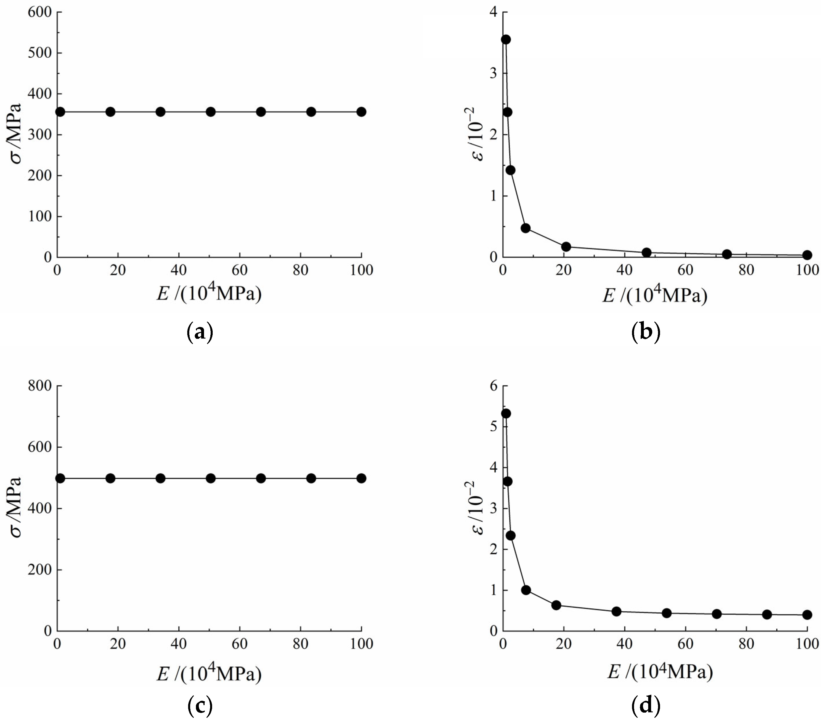
The effects of elastic modulus, yield strength, Poisson’s ratio, and other factors on stress–strain are studied, and then the decision variables and their value ranges are determined;

(3)

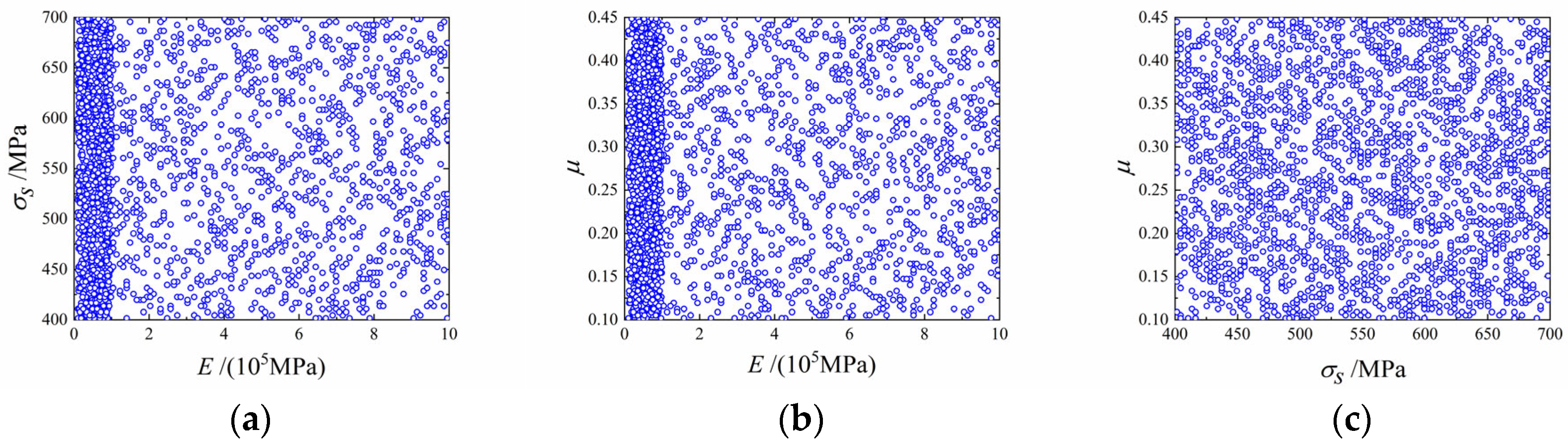
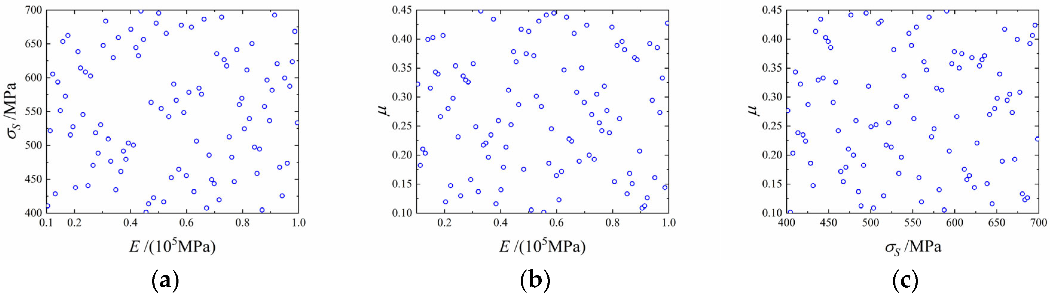
The method of random sampling is used to extract n groups of parameter combinations in the decision variable space;

(4)

The parameter combinations are substituted into finite element calculations to construct a sample set consisting of decision variables, stress and strain;

(5)

Based on the artificial neural network, the model of the mapping relationship between decision variables and stress and strain is trained separately;

(6)

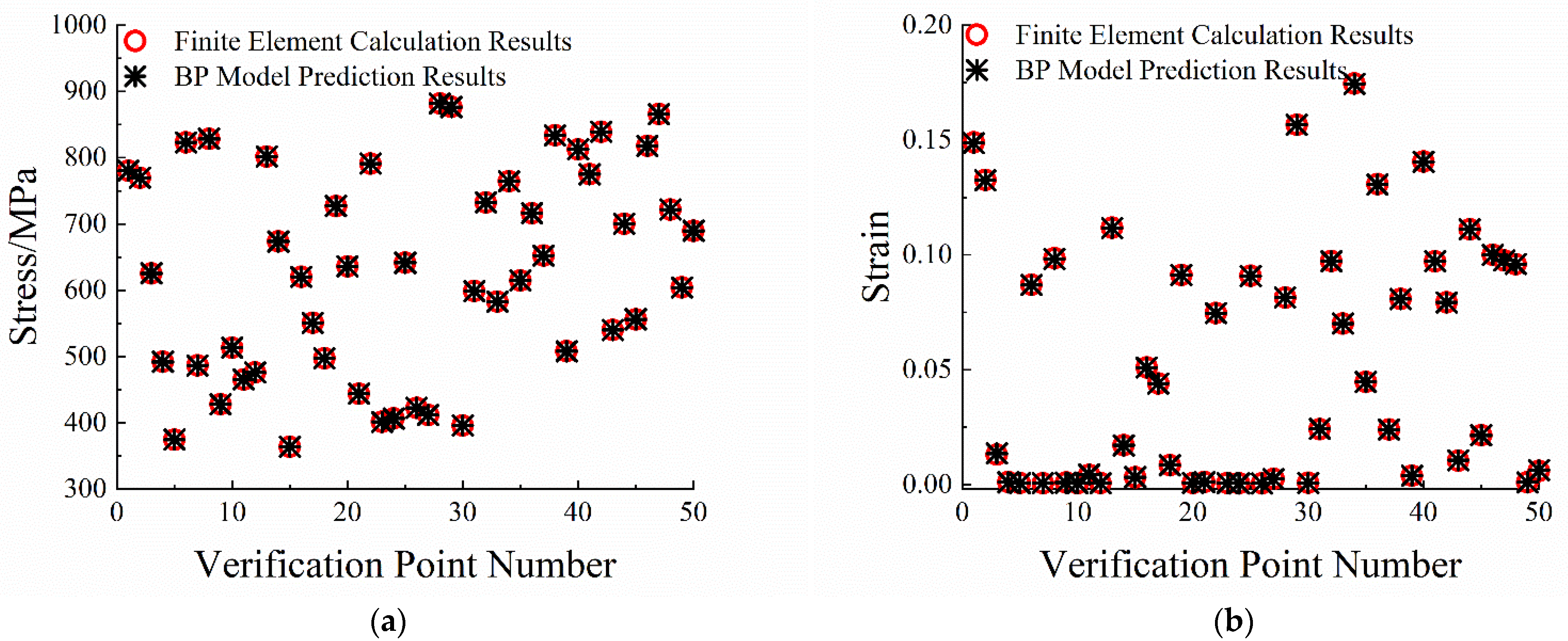
The mechanical behavior is predicted with the established model, and the reliability of the model is verified by finite element calculation and experimental data.

3. Construction of Mechanical Behavior Model of Materials

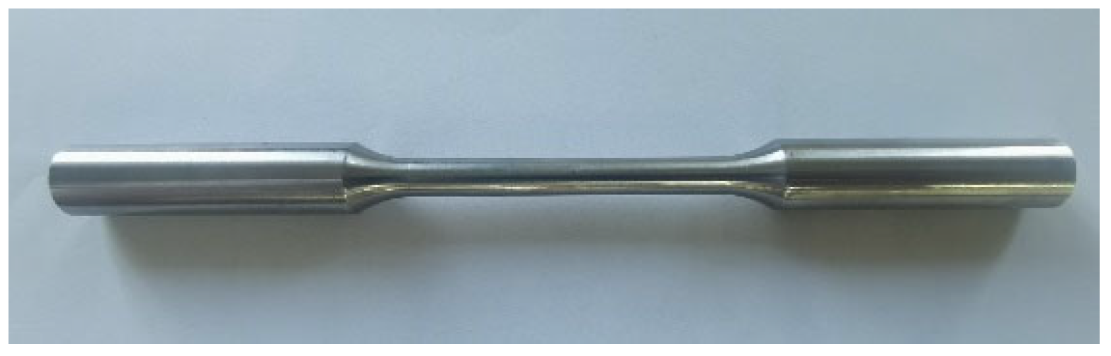
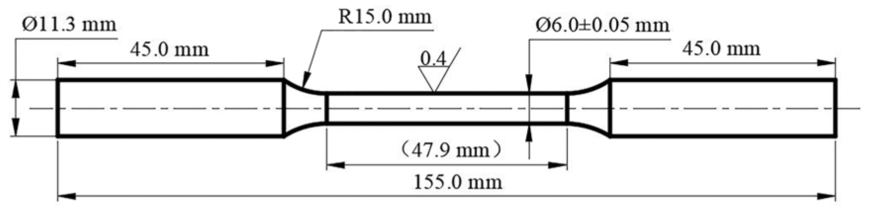
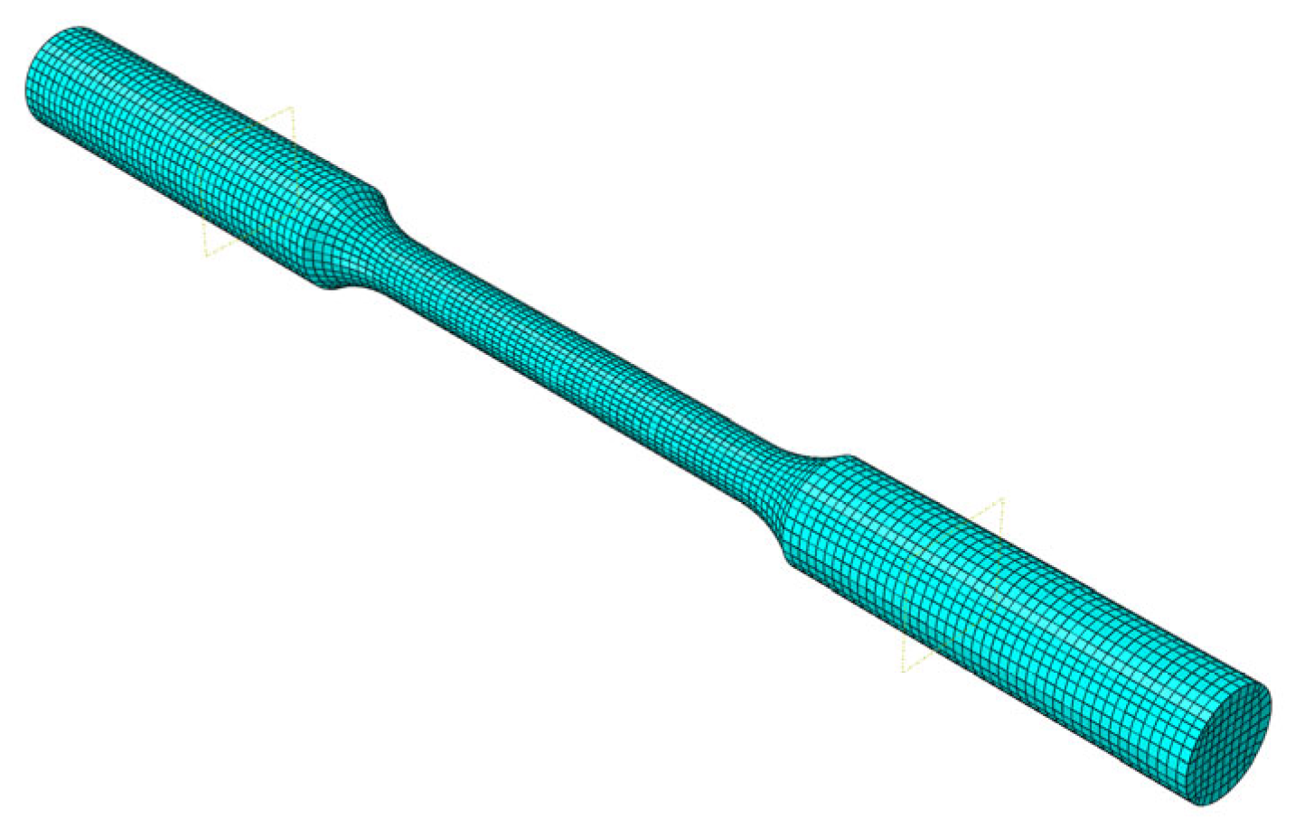
3.1. Establishing Finite Element Model

The geometric model of the quasi-static tensile specimen is established, using Solidworks software. The actual specimen is shown in Figure 2 and the specimen drawing is shown in Figure 3. Then, the model is imported into Abaqus for quasi-static tensile analysis. Considering that quasi-static tensile is a large deformation problem, geometric nonlinearity is turned on during calculation. After many comparisons, the grid size of the sample is set to 1 mm, which not only ensures the accuracy of finite element calculation but also reduces the calculation time. C3D8R solid element is selected to mesh the model, as shown in Figure 4, a total of 14,976 elements and 17,741 nodes are divided.

3.2. Influence Analysis of Material Parameters

In the elastic–plastic bilinear constitutive, the tangent modulus is used to define the mechanical properties of the material in the plastic stage. In this study, the tangent modulus is changed by changing yield strength and plastic point parameters, where the variable is reduced by changing only the plastic strain (${\epsilon }_{S1}$) corresponding to a given plastic stress (${\sigma }_{S1}$). The control variable method is used to analyze the influence of load ($F$), yield strength (${\sigma }_S$), elastic modulus ($E$), plastic strain (${\epsilon }_{S1}$) and Poisson’s ratio ($\mu$) on stress ($\sigma$) and strain ($\epsilon$). In order to accurately obtain the influence of each variable on the mechanical behavior of materials, the value range of each variable should be large enough. The value range of $F$ is 0~25,000 N, the value range of ${\sigma }_S$ is 400~700 MPa, the value range of $E$ is 1 × 10⁴~1 × 10⁶ MPa, the value range of ${\epsilon }_{S1}$ is 0.001~0.3, and the value range of $\mu$ is 0.1~0.45.

Taking $E$ as an example, the method of analyzing the influence of material parameters on stress and strain is illustrated. If the yield strength of the material is given, the material in the elastic stage or the plastic stage is affected by the amplitude of the load. To distinguish between the two stages, $F$ is given as 10,000 and 14,000, respectively, when calculating the elastic- and the plastic-phase laws. Only the elastic modulus is changed at each stage, and other parameters remain unchanged. Among them, $\mu$ is 0.33, ${\sigma }_S$ is 400 MPa, ${\sigma }_{S1}$ is 1000 MPa, and ${\epsilon }_{S1}$ is 0.0032. The $E-\sigma$ and $E-\epsilon$ curves are shown in Figure 5.

In Figure 5, in both stages, the stress does not change with the increase in $E$; the strain decreases with the increase in $E$, showing an inverse proportional trend. This method is used to obtain the influence law of $F$, ${\sigma }_S$, $E$, ${\epsilon }_{S1}$, and $\mu$ on $\sigma$ and $\epsilon$. The results show that the five variables have an influence on stress and strain, and the influence law of decision variables on stress and strain is monotonous.

3.3. Obtain Training Sample Set

A reasonable and effective data set is the premise and foundation of training an artificial neural network. In multidimensional continuous sample space, it is difficult to traverse all sample points, so it is necessary to discretize the multidimensional continuous parameter space reasonably. The core of reasonable discretization is to ensure that sample points uniformly fill the entire parameter space to fully represent the data characteristics of the entire sample space. In this paper, the Latin centroidal Voronoi tessellations (LCVT) sampling method [25] is used to sample decision variables in a continuous multidimensional space. In fact, in selecting sampling methods, a variety of methods can be compared and selected according to needs, not limited to the sampling method adopted in this paper.

As mentioned above, it is known that $F$, ${\sigma }_S$, $E$, ${\epsilon }_{S1}$, and $\mu$ have influence on the stress and strain, so five variables are used as decision variables. Considering the actual situation, the sampling range is consistent with that mentioned above. In the 5-dimensional space defined by the five value ranges, the 5-dimensional vector formed by each set of $F$, ${\sigma }_S$, $E$, ${\epsilon }_{S1}$, and $\mu$ is a group of decision variables. The LCVT sampling method is adopted to traverse the 5-dimensional space, and 2400 groups of decision variables are uniformly and randomly selected. For variables that span orders of magnitude, the method of sampling each order of magnitude is used to ensure that the variables can be uniformly sampled in each order of magnitude. The sampling groups are shown in

Table 1. Sampling groups.

Group Number	Quantity/Points	$\mathit{F}$/N	${\mathit{\sigma }}_{\mathit{S}}/\mathbf{MPa}$	$\mathit{E}$/MPa	${\mathit{\epsilon }}_{\mathit{S}1}$	$\mathit{\mu }$
1	100	0~100	400~700	1 × 104~1 × 105	0.001~0.01	0.1~0.45
2	100	0~100	400~700	1 × 104~1 × 105	0.01~0.1	0.1~0.45
3	100	0~100	400~700	1 × 104~1 × 105	0.1~0.3	0.1~0.45
4	100	0~100	400~700	1 × 105~1 × 106	0.001~0.01	0.1~0.45
5	100	0~100	400~700	1 × 105~1 × 106	0.01~0.1	0.1~0.45
6	100	0~100	400~700	1 × 105~1 × 106	0.1~0.3	0.1~0.45
7	100	100~1000	400~700	1 × 104~1 × 105	0.001~0.01	0.1~0.45
8	100	100~1000	400~700	1 × 104~1 × 105	0.01~0.1	0.1~0.45
9	100	100~1000	400~700	1 × 104~1 × 105	0.1~0.3	0.1~0.45
10	100	100~1000	400~700	1 × 105~1 × 106	0.001~0.01	0.1~0.45
11	100	100~1000	400~700	1 × 105~1 × 106	0.01~0.1	0.1~0.45
12	100	100~1000	400~700	1 × 105~1 × 106	0.1~0.3	0.1~0.45
13	100	1000~10,000	400~700	1 × 104~1 × 105	0.001~0.01	0.1~0.45
14	100	1000~10,000	400~700	1 × 104~1 × 105	0.01~0.1	0.1~0.45
15	100	1000~10,000	400~700	1 × 104~1 × 105	0.1~0.3	0.1~0.45
16	100	1000~10,000	400~700	1 × 105~1 × 106	0.001~0.01	0.1~0.45
17	100	1000~10,000	400~700	1 × 105~1 × 106	0.01~0.1	0.1~0.45
18	100	1000~10,000	400~700	1 × 105~1 × 106	0.1~0.3	0.1~0.45
19	100	10,000~25,000	400~700	1 × 104~1 × 105	0.001~0.01	0.1~0.45
20	100	10,000~25,000	400~700	1 × 104~1 × 105	0.01~0.1	0.1~0.45
21	100	10,000~25,000	400~700	1 × 104~1 × 105	0.1~0.3	0.1~0.45
22	100	10,000~25,000	400~700	1 × 105~1 × 106	0.001~0.01	0.1~0.45
23	100	10,000~25,000	400~700	1 × 105~1 × 106	0.01~0.1	0.1~0.45
24	100	10,000~25,000	400~700	1 × 105~1 × 106	0.1~0.3	0.1~0.45

. The extracted decision variables are successively put into the finite element model to calculate the corresponding $\sigma$ and $\epsilon$. The 7-dimensional vector formed by each group of $F$, ${\sigma }_S$, $E$, ${\epsilon }_{S1}$, $\mu$, $\sigma$, and $\epsilon$ is a sample point, and 2400 sample points constitute a sample set.

Take the three variables $E$, $\mu$, and ${\sigma }_S$ as examples to show the sampling results, as shown in Figure 6. The number of variable groups at each magnitude is the same in the sampling group; therefore, “local encryption” phenomenon is presented in the whole space. Still, the problem of not being able to extract data points from some regions in the whole space is solved. Meanwhile, for the independent 5-dimensional space of each group, the sampling distribution is uniform, which is illustrated by the three variables in the first group, as shown in Figure 7.

3.4. Obtain Mechanical Behavior Model

The artificial neural network has become an effective method to study the relationship between decision variables and objective function. A typical example is the back propagation (BP) neural network, a gradient descent learning algorithm based on the error back-propagation mechanism. According to the influence law of each decision variable on stress and strain, it is suitable to use BP neural network to establish a mapping relationship model. Based on BP neural network, the mapping relationship between decision variables and material stress and strain is constructed, which can be expressed as Equation (1):

$$\left\{\begin{array}{l}\sigma =f_{\sigma }(E,\mu ,{\sigma }_S,{\epsilon }_{S1},F)\\ \epsilon =f_{\epsilon }(E,\mu ,{\sigma }_S,{\epsilon }_{S1},F)\end{array}\right.$$

(1)

In the sample set, 50 groups of data are randomly selected as test samples, and other data were used as training samples. BP neural network is composed of input layer, hidden layer, and output layer. After many comparisons, it is determined that the neural network constructed by two hidden layers with neurons of 10 and 5, respectively, has the best effect. The schematic diagram of the network is shown in Figure 8. The training function of the network, the activation function of the hidden layer, and the activation function of the output layer are ‘tansig’, ‘tansig’, and ‘purelin’, respectively. The target error is 10⁻⁸, the learning rate is 0.005, and the maximum number of iterations is 1000. Thereby, the mapping relationship model is obtained. The mapping relationship model is used to predict the mechanical behavior and compare it with the actual value to verify the accuracy of the model, as shown in Figure 9.

Figure 9 shows that the prediction results of the two models are in good agreement with the finite element calculation results. In order to further verify the generalization ability of the BP neural network model, the model is used to predict the influence law of five decision variables on stress and strain, and the comparison is made with the actual law. Taking $E$ as an example, the result is shown in Figure 10.

Figure 10 shows that the predicted values of the model are consistent with the actual finite element results, and other parameters are verified by the same method. The results show that the training models have good generalization ability, and the influence law of each variable can be well predicted by the stress and strain models.

4. Verification of Mechanical Behavior Model

Non-dominated sorting genetic algorithm-II (NSGA-II) is a kind of genetic algorithm based on multiobjective optimization, which has advantages in calculating multiobjective optimization problems [26]. Since there are two objectives to be optimized, the NSGA-II algorithm is selected to verify the mechanical behavior model in this paper. The absolute value of the minimum value of the difference between the predicted stress and the experimental stress is defined as the objective function $f_{\sigma }$; the absolute value of the minimum value of the difference between the predicted strain and the experimental strain is defined as the objective function $f_{\epsilon }$, as shown in Equation (2):

$$\left\{\begin{array}{l}{f}_{\sigma }=\left|\min (sim(ne{t}_1,(E,\mu ,{\sigma }_S,{\epsilon }_{S1},P))-\sigma )\right|\\ f_{\epsilon }=\left|\min (sim(ne{t}_2,(E,\mu ,{\sigma }_S,{\epsilon }_{S1},P))-\epsilon )\right|\end{array}\right.$$

(2)

The NSGA-II optimization parameters are set to crossover probability 0.9, mutation probability 0.1, population size 100, maximum evolutionary generation 100, tournament size 2, crossover distribution index 20, and mutation distribution index 20. Then, the objective function constructed by the experimental data is solved. The solution parameters are back-substituted into the finite element model and compared with the quasi-static tensile experimental data of 9310 steel. The quasi-static tensile test is completed by using an MTS-880/25T electro-hydraulic servo universal testing machine, the maximum loading load of this universal testing machine is 250 KN. During the experiment, the upper chuck of the tensile machine is fixed, and the specimen is loaded at a constant speed by controlling the moving speed of the lower chuck. A strain gauge of type TA120-3AA is pasted at the geometric center of the specimen, the lead wire of the strain gauge and the lead wire of the testing machine are connected to the terminal. The stress and strain of the specimen during the tensile process are recorded simultaneously and in real-time, and then the experimental data are processed to obtain the stress–strain curve.

The verification results are shown in Figure 11, and the errors between the simulation results and the experimental data are shown in

Table 2. Errors between simulation results and experimental data.

Numbering	Simulation Stress/MPa	Experimental Stress/MPa	Error/%	Simulation Strain	Experimental Strain	Error/%
1	125.832	125.831	−0.00079	0.00036	0.00036	0
2	174.898	174.926	0.016007	0.00061	0.00061	0
3	275.920	275.988	0.024639	0.00109	0.00111	1.801802
4	375.948	374.948	−0.2667	0.00154	0.00156	1.282051
5	475.389	475.308	−0.01704	0.00210	0.00213	1.408451
6	526.049	525.967	−0.01559	0.00244	0.00248	1.612903
7	600.982	600.924	−0.00965	0.00390	0.00391	0.255754
8	695.248	695.283	0.005034	0.02975	0.03005	0.998336
9	705.428	705.461	0.004678	0.03618	0.03619	0.027632
10	714.968	715.007	0.005454	0.04421	0.04424	0.067812

. Among them, the error is calculated based on the experimental data.

Table 2 shows that the simulation results are in good agreement with the experimental stress and strain. The stress error is within 1%, and the strain error is within 2%. The results show that the mechanical behavior model of 9310 steel constructed by the BP neural network is highly reliable, and the method is feasible.

5. Conclusions

In this work, a prediction model of material mechanical behavior is established by combining artificial neural network, LCVT sampling algorithm and finite element calculation. The quasi-static tensile test of 9310 steel is taken as an example, and the performance of the mechanical behavior model is verified. The results show that the simulation results are in good agreement with the experimental results, and the error between the simulation results and the experimental results is within 2%. This work shows that the model has high reliability.

This paper proposes a method and idea for building a mechanical behavior model of materials, which provides a reference for obtaining mechanical behavior of materials. This method has a certain universality in the construction of mechanical behavior model of materials, in which BP neural network algorithm and LCVT sampling method can be reasonably selected according to the influence law of material properties and decision variables on the objective function, which is not limited to the selection algorithm in this paper.

References

1. Li, Y.; Ji, H.; Cai, Z.; Tang, X.; Li, Y.; Liu, J. Comparative Study on Constitutive Models for 21-4N Heat Resistant Steel during High Temperature Deformation. Materials 2019, 12, 1893–1915. [Google Scholar] [CrossRef] [Green Version]
2. Bobbili, R.; Madhu, V. Constitutive modeling and fracture behavior of a biomedical Ti–13Nb-13Zr alloy. Mater. Sci. Eng. A 2017, 700, 82–91. [Google Scholar] [CrossRef]
3. Salvado, F.C.; Teixeira-Dias, F.; Walley, S.M.; Lea, Lewis, J.; Cardoso, J.B. A review on the strain rate dependency of the dynamic viscoplastic response of FCC metals. Prog. Mater. Sci. 2017, 88, 186–231. [Google Scholar] [CrossRef] [Green Version]
4. Xin, X.; Zhao, W.; Xie, T. Analysis of compressive stress-strain curve of TB8 titanium alloy at room temperature. Forging and Stamping Tecnology. Forg. Stamp. Tecnol. 2014, 39, 126–130. [Google Scholar]
5. Cheng, Y.; Liu, J.; Pan, J.; Meng, L.; Wang, H.; Mao, H.; Yang, J. Test method for obtaining dynamic mechanical parameters of metallic materials. China Meas. Test 2016, 42, 107–112. [Google Scholar]
6. Gardner, L.; Yun, X. Description of stress-strain curves for cold-formed steels. Constr. Build. Mater. 2018, 189, 527–538. [Google Scholar] [CrossRef]
7. Kweon, H.D.; Kim, J.W.; Song, O.; Oh, D. Determination of true stress-strain curve of type 304 and 316 stainless steels using a typical tensile test and finite element analysis. Nucl. Eng. Technol. 2021, 53, 647–656. [Google Scholar] [CrossRef]
8. Zhao, K.; Wang, L.; Chang, Y.; Yan, J. Identification of post-necking stress–strain curve for sheet metals by inverse method. Mechanics of Materials. Mech. Mater. 2016, 92, 107–118. [Google Scholar] [CrossRef]
9. Rickman, J.M.; Lookman, T.; Kalinin, S.V. Materials informatics: From the atomic-level to the continuum. Acta Mater. 2019, 168, 473–510. [Google Scholar] [CrossRef]
10. Song, Z.; Chen, X.; Meng, F.; Cheng, G.; Wang, C.; Sun, Z.; Yin, W.-J. Machine learning in materials design: Algorithm and application. Chin. Phys. B 2020, 29, 116103–116132. [Google Scholar] [CrossRef]
11. Liu, Y.; Niu, C.; Wang, Z.; Gan, Y.; Zhu, Y.; Sun, S.; Shen, T. Machine learning in materials genome initiative: A review. J. Mater. Sci. Technol. 2020, 57, 113–122. [Google Scholar] [CrossRef]
12. Hart, G.L.W.; Mueller, T.; Toher, C.; Curtarolo, S. Machine learning for alloys. Nat. Rev. Mater. 2021, 6, 730–755. [Google Scholar] [CrossRef]
13. Cruz, D.J.; Barbosa, M.R.; Santos, A.D.; Miranda, S.S.; Amaral, R.L. Application of Machine Learning to Bending Processes and Material Identification. Metals 2021, 11, 1418–1442. [Google Scholar] [CrossRef]
14. Xie, J.; Su, Y.; Xue, D.; Jiang, X.; Fu, H.; Huang, H. Application of machine learning in material research and development. Acta Metall. Sin. 2021, 57, 1343–1361. [Google Scholar]
15. Zhang, J.M.; Yang, W.D.; Li, Y. Application of artificial intelligence in composite material research. Advances in Mechanics. 2021, 51, 865–900. [Google Scholar]
16. Naser, M.Z. Deriving temperature-dependent material models for structural steel through artificial intelligence. Constr. Build. Mater. 2018, 191, 56–68. [Google Scholar] [CrossRef]
17. Jang, D.P.; Fazily, P.; Yoon, J.W. Machine learning-based constitutive model for J2- plasticity. Int. J. Plast. 2021, 138, 102919–102939. [Google Scholar] [CrossRef]
18. Stoffel, M.; Bamer, F.; Markert, B. Artificial neural networks and intelligent finite elements in non-linear structural mechanics. Thin-Walled Struct. 2018, 131, 102–106. [Google Scholar] [CrossRef]
19. Stoffel, M.; Bamer, F.; Markert, B. Neural network based constitutive modeling of nonlinear viscoplastic structural response. Mech. Res. Commun. 2019, 95, 85–88. [Google Scholar] [CrossRef]
20. Sharath, B.N.; Venkatesh, C.V.; Afzal, A.; Aslfattahi, N.; Aabid, A.; Baig, M.; Saleh, B. Multi ceramic particles inclusion in the aluminium matrix and wear characterization through experimental and response surface-artificial neural networks. Materials 2021, 14, 2895–2919. [Google Scholar] [CrossRef]
21. Nagaraja, S.; Kodandappa, R.; Ansari, K.; Kuruniyan, M.S.; Afzal, A.; Kaladgi, A.R.; Aslfattahi, N.; Saleel, C.A.; Gowda, A.C.; Bindiganavile Anand, P. Influence of heat treatment and reinforcements on tensile characteristics of aluminium AA 5083/Silicon Carbide/Fly ash composites. Materials 2021, 14, 5261–5288. [Google Scholar] [CrossRef] [PubMed]
22. Wang, C.; Shen, C.; Cui, Q.; Zhang, C.; Xu, W. Tensile property prediction by feature engineering guided machine learning in reduced activation ferritic/martensitic steels. J. Nucl. Mater. 2020, 529, 151823–151842. [Google Scholar] [CrossRef]
23. Guo, S.; Yu, J.; Liu, X.; Wang, C.; Jiang, Q. A predicting model for properties of steel using the industrial big data based on machine learning. Comput. Mater. Sci. 2019, 160, 95–104. [Google Scholar] [CrossRef]
24. Merayo, F.D.; Rodríguez-Prieto, A.; Camacho, A.M. Prediction of the Bilinear Stress-Strain Curve of Aluminum Alloys Using Artificial Intelligence and Big Data. Metals 2020, 10, 904–933. [Google Scholar] [CrossRef]
25. Loyola, R.D.; Pedergnana, M.; Gimeno, G.S. Smart sampling and incremental function learning for very large high dimensional data. Neural Netw. 2016, 78, 75–87. [Google Scholar] [CrossRef] [PubMed] [Green Version]
26. Deb, K.; Agrawal, S.; Pratap, A.; Meyarivan, T. A fast elitist non-dominated sorting genetic algorithm for multi-objective optimization: NSGA-II. In Proceedings of the International Conference on Parallel Problem Solving from Nature, Paris, France, 18–20 September 2000; Springer: Berlin/Heidelberg, Germany, 2000; pp. 849–858. [Google Scholar]
Figure 1. Model construction method.
Metals 12 01086 g001
Figure 2. Tensile specimen.
Metals 12 01086 g002
Figure 3. Specimen size drawing.
Metals 12 01086 g003
Figure 4. Finite element model.
Metals 12 01086 g004
Figure 5. Influence law of E on stress and strain: (a) influence law of elastic stage E on stress; (b) influence law of elastic stage E on strain; (c) influence law of plastic stage E on stress; (d) influence law of plastic stage E on strain.
Metals 12 01086 g005
Figure 6. Sampling distribution of spatial variables: (a) E σ S ; (b) E μ ; (c) σ S μ .
Metals 12 01086 g006
Figure 7. Sampling results of the first group of three variables: (a) E σ S ; (b) E μ ; (c) σ S μ .
Metals 12 01086 g007
Figure 8. ANN structure diagram: (a) stress model structure diagram; (b) strain model structure diagram.
Metals 12 01086 g008
Figure 9. Mapping model validation: (a) stress model validation; (b) strain model validation.
Metals 12 01086 g009
Figure 10. Model validation of change E : (a) elastic stage E σ ; (b) elastic stage E ε ; (c) plastic stage E σ ; (d) plastic stage E ε .
Metals 12 01086 g010
Figure 11. Comparison of simulation results with experimental data.
Metals 12 01086 g011