On the Registration of Thermographic In Situ Monitoring Data and Computed Tomography Reference Data in the Scope of Defect Prediction in Laser Powder Bed Fusion

Abstract

The detection of internal irregularities is crucial for quality assessment in metal-based additive manufacturing (AM) technologies such as laser powder bed fusion (L-PBF). The utilization of in-process thermography as an in situ monitoring tool in combination with post-process X-ray micro computed tomography (XCT) as a reference technique has shown great potential for this aim. Due to the small irregularity dimensions, a precise registration of the datasets is necessary as a requirement for correlation. In this study, the registration of thermography and XCT reference datasets of a cylindric specimen containing keyhole pores is carried out for the development of a porosity prediction model. The considered datasets show variations in shape, data type and dimensionality, especially due to shrinkage and material elevation effects present in the manufactured part. Since the resulting deformations are challenging for registration, a novel preprocessing methodology is introduced that involves an adaptive volume adjustment algorithm which is based on the porosity distribution in the specimen. Thus, the implementation of a simple three-dimensional image-to-image registration is enabled. The results demonstrate the influence of the part deformation on the resulting porosity location and the importance of registration in terms of irregularity prediction.

1. Introduction

The industrial use of metal-based additive manufacturing (AM) processes has rapidly increased in recent years [1]. In comparison to traditional manufacturing, AM technologies such as laser powder bed fusion (L-PBF) offer the benefit of producing parts of highly complex geometry directly from the 3D CAD model while reducing the material waste [2]. L-PBF counts as one of the most established AM techniques and stands out due to its ability to produce features in high spatial resolution of tens of microns [3,4]. However, the occurrence of irregularities such as internal porosity, cracks, or surface roughness during manufacturing poses a risk to the final component quality [4,5]. Poor process parametrization (i.e., by scan velocity and laser power) was found to be an influential factor for the formation of irregularities [5]. Thermography as a radiometric nondestructive testing method has been utilized to monitor the part’s local thermal history. This is performed by extracting thermal features from the spatial and temporal temperature distribution of the melt pool and part surface. From the obtained feature distribution, local areas of thermal deviation can be identified in which porosity is likely to form [6]. As a reference technique for the determination of the spatial distribution of porosity, X-ray micro computed tomography (XCT) is widely applied [7]. The correlation of thermographic feature data and XCT reference data facilitates the prediction of porosity likelihood [6]. The in situ detection of porosity has received increasing attention in the scientific community in recent years which is evident from the rising number of publications [8].

An important aspect for the prediction of irregularities such as porosity is the registration of the in situ monitoring and the reference XCT data. Image registration can be understood as the spatial alignment of two or more images. This mainly includes the goal of finding a transformation that aligns the features of interest visible in the image data [9]. A registration function can be obtained by applying a spatial transformation on a moving image that is registered with a fixed image. Here, a similarity measure or a cost function between the two images is optimized typically in several iteration steps [10,11]. A common example of a registration function is the affine transformation model, which allows translation, rotation, scaling, and skew of the moving image. This high number of degrees of freedom with respect to image transformation is not always necessary. For many applications, it might be sufficient to utilize only a rigid model that allows translation and rotation [11]. The evaluation of the registration accuracy is challenging and often limited to a qualitative validation by the user [12].

In terms of predicting internal porosity from sensor data, methods of artificial intelligence such as machine learning (ML) algorithms can be applied [13]. A requirement for a successful prediction is the accurate spatial allocation between sensor signal and resulting porosity information. Otherwise, the model is trained on spatially mismatched data and basically learns irrelevant data patterns. In L-PBF, the occurring irregularities have small dimensions. For example, in a study by Sinclair et al. [14], keyhole pores with diameters in the range of 10–60 μm were quantified. From that, it can be concluded that for a prediction of single keyhole pores, even small allocation errors resulting from the registration may significantly reduce the performance of the prediction model.

Furthermore, the differences in data format and dimensionality resulting from the different measurement methods are challenging for registration. The layer-wise acquired thermograms from in situ thermography contain information about the thermal radiation from the different object surfaces visible in the field of view of the camera (i.e., melt pool, solidified material, unmolten powder, and machine surroundings) [15]. Due to the projection of the 3-dimensional (3D) scene to the 2-dimensional (2D) focal plane array of the camera sensor, the height information of the specimen surface is lost. Thermographic in situ monitoring in L-PBF will result in 4-dimensional (4D) data consisting of a time series of 2D thermograms for each manufactured layer. Here, the measurable signal is limited by the camera dynamics as well as the chosen spatial and temporal resolution. In contrast, XCT provides a spatially high resolved 3D object representation of the manufactured specimen. The 3D object reconstruction is created from 2D projection images captured by a flat panel X-ray detector. The projection images are reconstructed using algorithms such as the Feldkamp algorithm for cone beam geometry [16]. The reconstruction includes an interpolation process on the gray value voxel grid. Artifacts, such as scatter [17], cone beam [18], and beam hardening [19], may decrease the spatial resolution and the registration procedure. Furthermore, the XCT data contains all shape deformations of the part caused by the manufacturing process which remain in the part after removal from the dummy cylinder, such as shrinkage and warping [20].

In the literature [6,8,21,22,23,24,25,26,27], a range of methods is utilized to align thermographic in situ monitoring data and XCT reference data as a preparational step for irregularity prediction in the scope of L-PBF. Here, the insertion of artificial voids offers the advantage of predefined void location and shape. This benefits the identification of the defects in the determined in situ signal [8]. Mireles et al. [21] integrated artificial voids in the design of a metal part manufactured by electron beam melting. The correlation between reference XCT data and data obtained by an off-axis infrared (IR) camera was performed utilizing the known defect position within the part. Lough et al. [22] qualitatively compared single lateral slices in a cylindrical test specimen on the basis of voids that were produced by decreasing the laser power. In a study by Coeck et al. [23], the registration of IR data and XCT data was performed utilizing the large size of the present lack of fusion (LoF) voids in the observed specimen as reference object. Due to the low number of voids (45 voids in a 10 mm³ volume) and their large dimensions, a straightforward spatial assignment between voids and melt pool monitoring data was feasible. The data time series derived from the off-axis photodiodes of the melt pool monitoring system were mapped to the 3D position of the laser scanner. Single data points from the obtained point cloud were allocated to a void event if the distance between the data point centroid and the void centroid was below 500 μm. Forien et al. [24] overlapped X-ray radiography scans of single tracks with coaxial pyrometry in situ monitoring data using a manual translation. Like [23], the time series data obtained by pyrometry was mapped to the 3D laser scanner position. Voids were segmented manually and correlated with the pyrometry signal in a radius of 65 μm around the void centroids.

Apart from manual mapping of signal and reference data, image registration algorithms can be utilized to automatically align multiple images for further analysis [9]. A 3D image registration was performed by Mohr et al. [25] to overlap optical tomography and XCT datasets. Here, the open-source software elastix 4.9 (University Medical Center Utrecht, Utrecht and contributors, The Netherlands) was utilized to apply an affine transformation. In a recently published study, Lough et al. [6] performed a voxel-based quantitative analysis using a layer-by-layer registration along the z axis of the specimen which included down-sampling of the XCT dataset. Here, the datasets were aligned manually along the z axis. Afterwards, an automated translation algorithm was applied. Taherkani et al. [26] registered XCT data according to the specimens CAD file using the 3D image analysis software Dragonfly Pro v4.0 (Object Research Systems Inc., Montreal, QC, Canada). As geometric reference, horizontal and vertical grooves were integrated into their specimen design. The alignment of the CT data with the melt pool monitoring data was carried out on the basis of artificial voids integrated in the specimen. Gobert et al. [27] utilized an affine mapping function to register CT data and powder bed image data acquired by a high resolution digital single-lens camera. The registration was based on minimization of the root mean square error between geometrical reference points in the datasets.

The literature [4,5] emphasizes that irregularity prediction in L-PBF is an important task to predict the service life of the produced part. The development of accurate prediction models requires a precise image registration of the acquired monitoring data and the reference data, especially due to the small dimensions of the occurring irregularities. To the authors’ knowledge, few systematic investigations concerning registration methods in the scope of irregularity prediction in L-PBF have been performed. Some authors [21,22] rely on large artificial voids integrated in the specimen design to simplify their detection in the sensor data and in the ground truth data. If registration algorithms are applied, their accuracy is usually not further specified, even though it is essential information to evaluate the measurement uncertainty. Furthermore, the influence of occurring shape distortions such as warping or shrinkage in the datasets are usually not included in the registration approach.

This study focuses on the registration of feature datasets extracted from in situ thermography and an XCT dataset of a cylindric specimen that contained keyhole pores [28]. The registration is performed as a preliminary step to facilitate a highly accurate prediction of the present irregularities using ML methods (to be reported in a sister paper). The introduced registration methodology focuses on dataset preprocessing to enable the application of a simple 3D image-by-image registration. A systematic description of the singular data processing steps and the challenges arising from the different formats and dimensionalities of the datasets is given. In the context of the XCT dataset, especially the influence of the present shrinkage and material elevation on the registration accuracy is examined. Here, a novel method to adaptively adjust the part deformation is developed based on the pore distribution in the specimen. The obtained registration accuracy is evaluated and future challenges in the context of irregularity prediction in L-PBF are derived.

2. Materials and Experimental Procedures

A cylindrical specimen was produced on a commercial L-PBF machine (SLM 280 HL, SLM Solutions Group AG, Lübeck, Germany) using AISI 316L stainless steel powder. The powder was specified as follows: apparent density of 4.58 g/cm³, D_mean = 34.69 μm, D₁₀ = 18.22 μm, D₅₀ = 30.5 μm, and D₉₀ = 55.87 μm. The specimen design included a surrounding staircase structure as registration landmark (see Figure 1) inspired by a study by Gobert et al. [27]. The entire specimen was built upon the milled surface of a dummy cylinder to prevent cutting losses. The inner cylinder (diameter: 7 mm, height: 12 mm) consisted of six sections. The sections were manufactured with varying processing parameters to introduce keyhole porosity into the material. The parameter variation was performed by decreasing the scanning velocity. This resulted in increased volumetric energy densities (VED) [28], see

Table 1. Overview of the manufacturing conditions of the different cylinder sections (corresponding to specimen “B” in [28]). In the last column, the relative increase of the VED in comparison to sections 1, 3, and 5 is given by the percentage value in brackets.

Section	Layer Count	Laser Power P in W	Scan Velocity v in mm/s	VED in J/mm3
1	1–60	275	700	65.45
2	61–80	275	560	81.84 (+25%)
3	81–140	275	700	65.45
4	141–160	275	467	98.21 (+50%)
5	161–220	275	700	65.45
6	221–240	275	400	114.45 (+75%)

. A hatch distance of 120 μm and a layer thickness of 50 μm were utilized. Furthermore, a cross and a letter landmark were added to the specimen’s top surface as further geometric landmarks.

The in situ monitoring setup consisted of three infrared cameras that were mounted off-axis outside of the machine, utilizing a custom-made optical entrance. The thermal radiation of the process was guided to the cameras by a system of gold-coated mirrors and beam splitters that were optically adapted to the spectral sensitivity of the respective camera system. For further details concerning the powder specifications, scanning strategy, and the machine setup, refer to a previously conducted study [28]. In this study, the in situ monitoring data of the deployed short-wave infrared camera (Goldeye CL-033 TEC1 from Allied Vision Technologies GmbH, Stadtroda, Germany) was utilized for the investigation.

From the short-wave infrared camera, a 4D dataset consisting of thermograms with the size of 90 pix² (pixel scale of approximately 100 μm/pix) was obtained from 240 manufacturing layers during the process monitoring. The dataset size was 90 × 90 × n_im,l × 240, where n_im,l depicts the number of the image that was acquired during the exposure of a single layer l. n_im,l could vary slightly for the different layers due to variations in the starting time of the recording and durations of the layer illumination. It was of the order of approximately 8000 images. All thermograms were temperature calibrated using a single point calibration method [29]. Ten different features were identified from the spatial and temporal temperature information present in the thermograms (

Table 2. Extracted features from in-situ monitoring thermograms.

Feature Class	Feature
Melt pool-based features 1	Area
	Length
	Width
	Eccentricity
	Perimeter
	Mean temperature
	Maximum temperature
Time-dependent temperature features	Time over threshold of 1200 K
	Time over threshold of 1680 K
	Time over threshold of 2400 K

¹ Corresponding to the geometry and temperature distribution of the apparent melt pool blob visible in the thermogram data.

). Detailed insights concerning the feature extraction can be found in [28]. A coordinate system S (Figure 1) was introduced to describe the respective 3D voxel position of each feature value in the specimen data. The features were distinguished into melt pool-based and time-dependent temperature features. Both feature classes differed in spatial information density. Melt pool-based features were extracted for each image and spatially assigned to the x-y position of the pixel with the highest temperature visible in the image. This pixel represented the position where the laser spot was located on the specimen surface. Due to the temporal and spatial resolution of the camera, the melt pool feature data were distributed sparsely in each respective layer. The sparsity was dependent on the scan velocity and resulted in data point distances along a single scan track ranging from approximately 110 μm (in section 6) to 200 μm (in sections 1, 3, and 5) with a hatch distance of 120 μm. The feature extraction resulted in 3D datasets Fⁱ of the size 3 × n_mp,l × 240. Here, the first dimension represented the individual feature value and its associated x-y position in the observed layer (in total 240 layers). The index i in Fⁱ corresponds to the observed melt pool feature and n_mp,l corresponds to the number of melt pool images in the image series of the respective layer. The time-dependent features were calculated from the temporal temperature information of each image pixel from a single layer manufacturing. Hence, the spatial information density was limited only by the spatial resolution of the camera. As a result, 3D datasets F^j of the size 90 × 90 × 240 were generated for the respective time-dependent feature j. According to the spatial resolution of the camera and the nominal layer height, a voxel size of 100 × 100 × 50 μm³ was present in all datasets.

Subsequent to manufacturing, XCT was performed on the specimen and the surrounding staircase after separation from the base plate using the commercial CT-scanner GE v|tome|x 180/300 (GE Sensing and Inspection Technologies GmbH, Wunstorf, Germany) [28]. A voltage of 222 kV and a current of 45 μA were used to acquire 3000 projections at an acquisition time of 2 s. To improve the signal-to-noise ratio of the projections, three images were taken at each of the 3000 angular positions, and their average was used for the 3D reconstruction. The reconstruction of the XCT projection data was performed by using the filtered back-projection algorithm [16], resulting in a raw dataset V^raw with the spatial dimension of 2024 × 2024 × 2024 and a voxel size of 10 μm³. The achieved voxel size enabled the quantitative analysis of features of a size above 20 μm³. A further coordinate system S′ (Figure 1) given by the axis of the original XCT data was utilized to describe the XCT voxel positions. Subsequent to the reconstruction, a beam hardening correction [30] was performed. Furthermore, the cylinder axis was aligned parallel to the z′ axis. This was carried out using ImageJ Fiji [31] and MATLAB (MathWorks Inc., Natick, MA, USA). Here, contiguous x′-y′ slices were extracted from V^raw and a circle fit [32] was applied to the circular shape visible in the slice. Afterwards, the circle fit centroids of all slices were calculated. From the calculated course of the centroids along the z′ axis, the angle of cylinder axis inclination was determined. The alignment was performed by manual rotation of the cylinder around the x′ and y′ axis. The resulting angle deviation after the axis alignment was calculated to approximately 0.005°. This resulted in a maximum height deviation at the specimen surface of approximately 1 μm (regarding height and diameter of the CAD of the specimen). The image data were further processed by adjusting the brightness and the contrast. A 3D dataset V^proc with the size of 711 × 711 × 1260 voxels was obtained containing the density information of inner cylinder and the landmark structures on the specimen top. In the following, a local thresholding algorithm introduced by Phansalker et al. [33] was applied to the data to distinguish between material and voids. The binarized dataset is denoted as V^proc,bin. An overview of the datasets that are used in this study is given in

Table 3. Overview of the obtained datasets from thermography and XCT. n_mp,l corresponds to the number of images acquired during the manufacturing of a single layer and is in the order of approximately 8000 images.

Dataset	Source	Content	Dimensions	Voxel Size in μm3
Fi	SWIR camera	Values of i-th melt pool-based feature	3 × nmp,l × 240	100 × 100 × 50
Fj	SWIR camera	Values of j-th time-dependent temperature features	90 × 90 × 240	100 × 100 × 50
Ak	SWIR camera	Preprocessed and interpolated values of k-th feature	935 × 980 × 1200	10 × 10 × 10
Vraw	XCT	Density information (raw)	2024 × 2024 × 2024	10 × 10 × 10
Vproc	XCT	Density information (cropped, increased contrast)	711 × 711 × 1260	10 × 10 × 10
Vproc,bin	XCT	Porosity information (cropped)	711 × 711 × 1260	10 × 10 × 10
Vfinal	XCT	Porosity information (cropped, adjusted to CAD)	711 × 711 × 1200	10 × 10 × 10

.

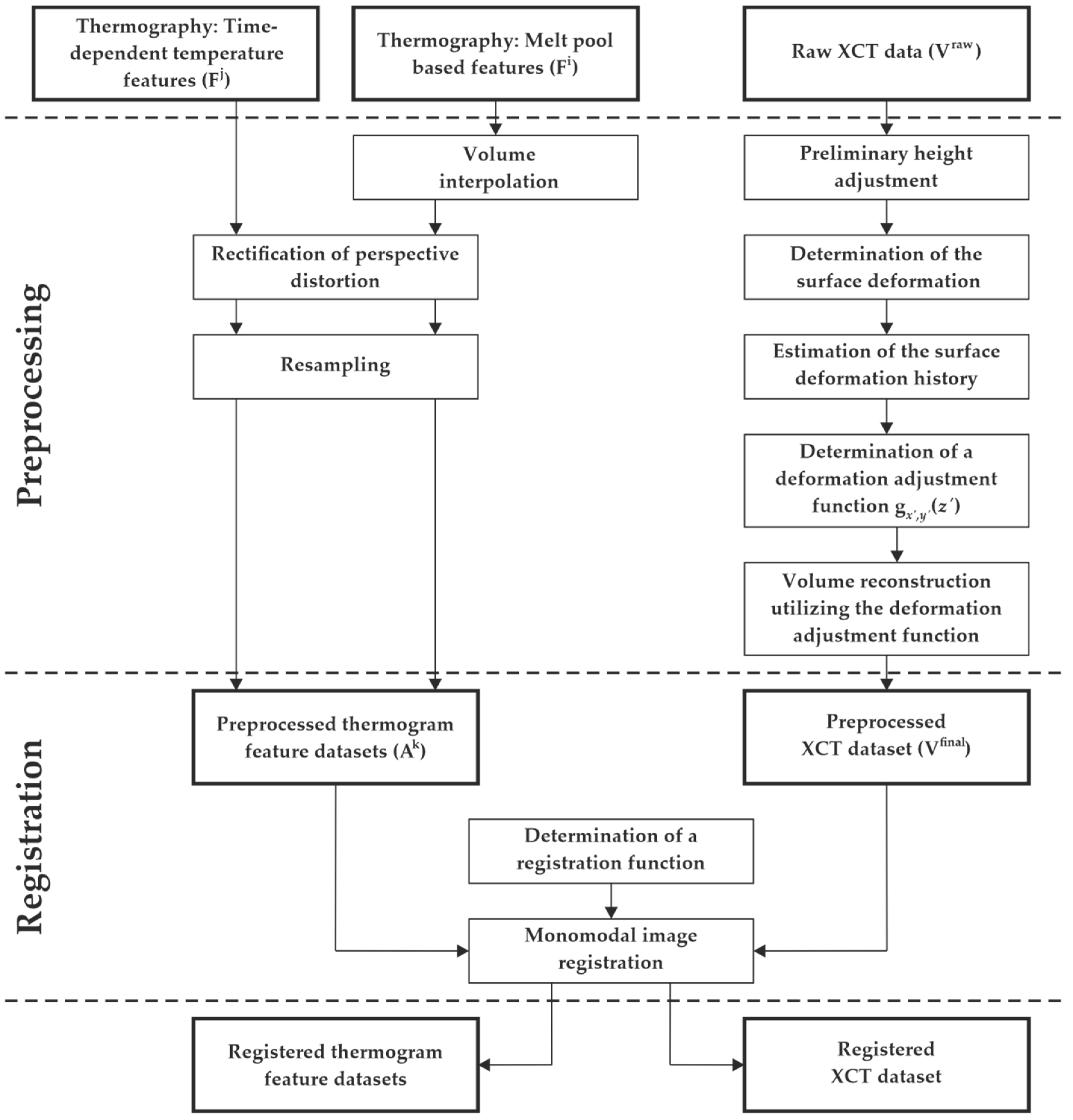
3. Registration Methodology and Results

The aim of this study was the registration of the obtained thermogram feature datasets and the corresponding XCT dataset to produce an accurately aligned data basis for future irregularity prediction modeling. Preprocessing methods were used to adjust each dataset to match the original specimen geometry given by the CAD. Based on a sophisticated preprocessing workflow, the registration was simplified to a simple 3D image-to-image algorithm. In the following, the performed processing steps concerning thermogram feature data, the reference XCT data, and the image registration are described, and the obtained results are presented. A schematic overview of all performed steps is given in Figure 2.

3.1. Preprocessing of Thermogram Feature Dataset

A first evaluation of the obtained melt pool-based feature dataset Fⁱ and the time-dependent feature dataset F^j revealed three pre-registration challenges: First of all, due to the sparse nature of Fⁱ, a volume interpolation was necessary to perform an image-to-image registration [34]. Secondly, perspective distortion was found in both datasets resulting from the optical setup [28] used for the process monitoring. Such distortion led to inconsistent voxel scales in the x and y axis. Thirdly, the datasets were resampled to the voxel scale 10 μm³ of the XCT reference data to enable the precise spatial overlap of all datasets. One 3D linear interpolation algorithm was implemented to solve all three pre-registration challenges. Thus, missing pixel values in the sparse melt pool-based features were interpolated (see Figure 3a), the present imaging error was rectified, and the voxel size was adjusted. The distorted image scales s_x = 103.8 μm/pix and s_y = 108.9 μm/pix were calculated from pre-manufacturing recordings of a calibration target (grid pattern), while the scale in the z direction s_z was given by the layer thickness of 50 μm. The size of the rectified target volume A (width w_A, depth d_A, and height h_A) was derived from the former thermogram size 90 pix² and the overall layer count (240 layers):

$${\mathrm{w}}_{\mathrm{A}}=90·\frac{{\mathrm{s}}_{x^{\prime }}}{{\mathrm{s}}_x}$$

(1)

$${\mathrm{d}}_{\mathrm{A}}=90·\frac{{\mathrm{s}}_{y^{\prime }}}{{\mathrm{s}}_y}$$

(2)

$${\mathrm{h}}_{\mathrm{A}}=240·\frac{{\mathrm{s}}_{z^{\prime }}}{{\mathrm{s}}_z}$$

(3)

Here, ${\mathrm{s}}_{x^{\prime }}$ = 10 μm, ${\mathrm{s}}_{y^{\prime }}$ = 10 μm and ${\mathrm{s}}_{z^{\prime }}$ = 10 μm denote the voxel size of the XCT data.

From the initial datasets Fⁱ and F^j, k = i + j = 10 datasets A^k with a size of 935 × 980 × 1200 voxels were interpolated. The results of the interpolation of melt pool-based feature data from a single layer are depicted in Figure 3b.

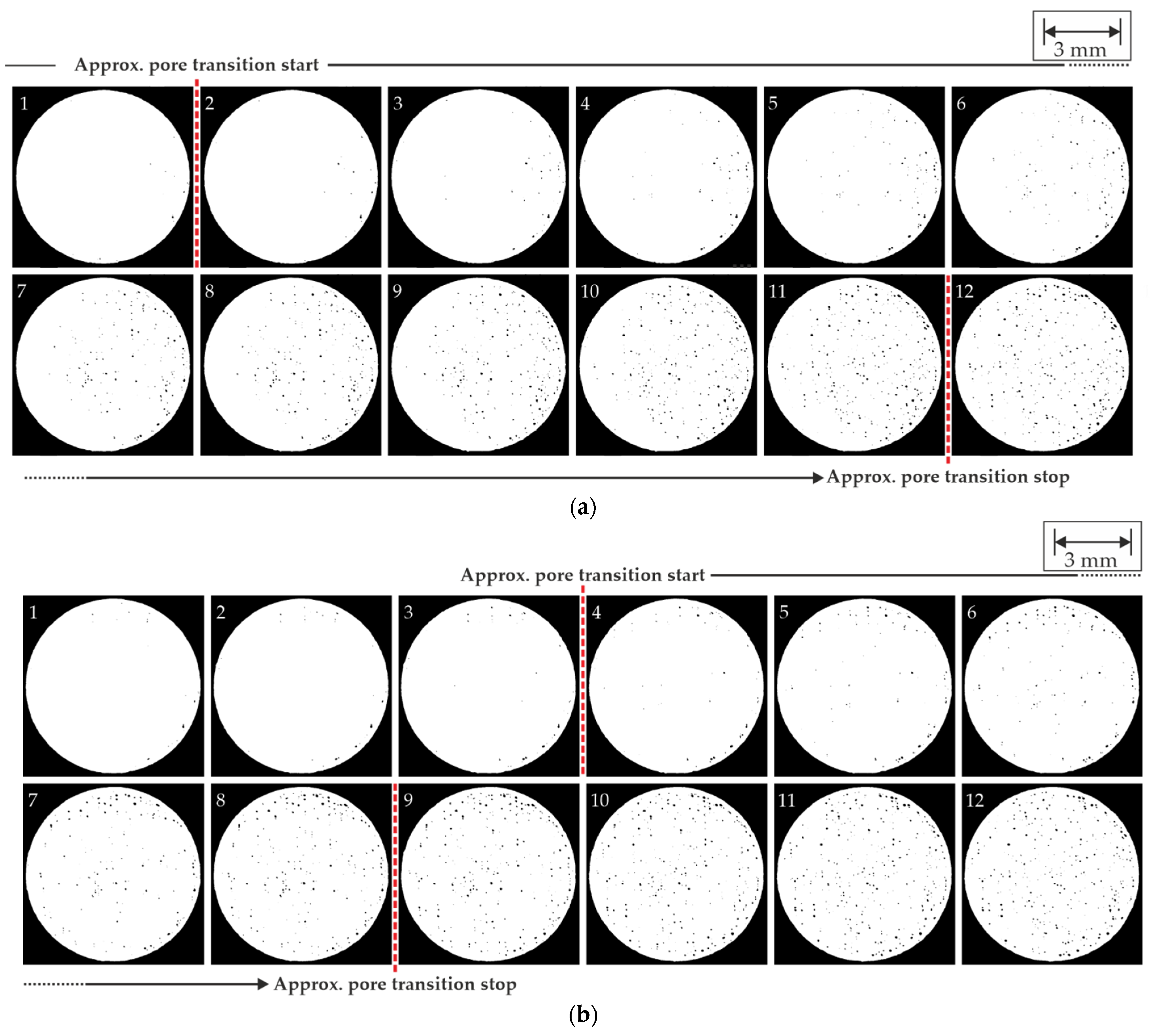
3.2. Preprocessing of XCT Dataset

The XCT dataset contained the porosity information present in the specimen. The dimensions and the shape of the cylindric specimen in the XCT dataset deviated significantly from the shape of the original CAD. A first comparison of the specimen to the CAD model height showed a vertical shrinkage. Furthermore, the observation of the top surface revealed a severe shape deformation. The surface rim was elevated in comparison to its center. This resulted in significant height deviations (see Figure 4). The maximum height differences of approximately 400 μm between surface rim and center (which corresponds to 8 manufacturing layers) would produce major errors if a simple lateral slicing along the x′-y′ plane was performed for correlation with the monitoring data. Alongside this, the registration landmarks (letter and cross) that were later utilized to obtain a registration function were inspected since they can be clearly separated from the main cylindrical specimen. The bordering areas of the landmarks exhibited a local height increase. This represented a distortion of the original surface (see Figure 4). The surface deformation posed a major difficulty for the registration because it was unclear how the deformation was formed over the course of the manufacturing process.

Ulbricht et al. [7] found a similar surface deformation in an equally designed specimen that was manufactured using the same material and machine. Furthermore, they found indications of a comparable surface deformation at multiple stages of the manufacturing process. These previous deformations were estimated from the observation of LoF voids at the transition from a void-free section and followed by a section with artificial voids (notches) within the specimen. The authors suggested that the deformation could have been present during the entire manufacturing process. In the current study, the observation of the pore distribution in the transition from section 5 to 6 indicated a similar effect (see Figure 4). Therefore, a method was developed to adjust the surface in the dataset based on the deformation information obtained from the pore distribution. The method assumed that all previous surface deformations that had formed during manufacturing had a qualitatively similar shape to the visible deformation of the specimen surface. Furthermore, it was assumed that the previous surface deformation can be reconstructed from the depth distribution of the lowest keyhole pores at the onset of a region with increased VED, i.e., section 6. Finally, the preprocessing method for the XCT dataset consisted of five steps (compare Figure 2):

• Preliminary height adjustment;
• Determination of the surface deformation;
• Estimation of the surface deformation history;
• Determination of a deformation adjustment function;
• Volume reconstruction utilizing the deformation adjustment function.

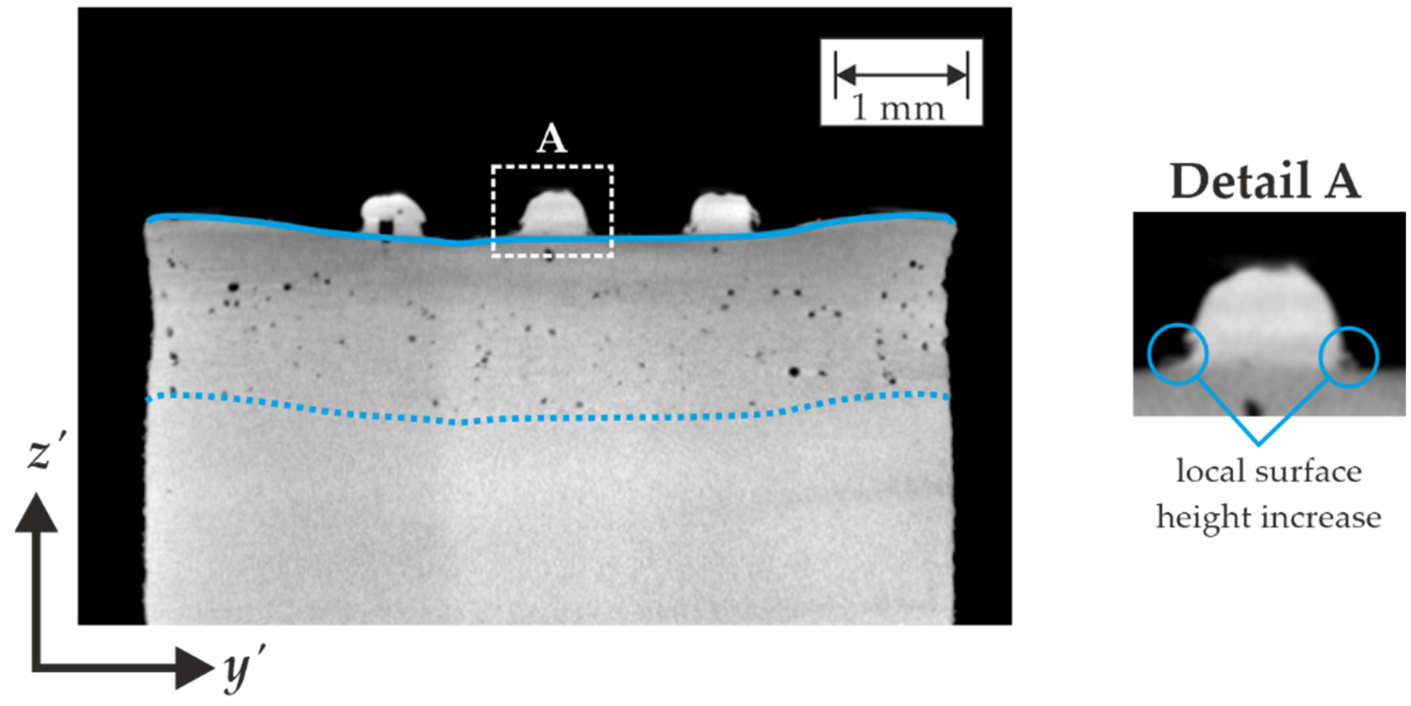
3.2.1. Preliminary Height Adjustment

Due to the height difference between the manufactured specimen represented in the XCT dataset and the original CAD, a preliminary height adjustment was performed. The shrinkage was estimated from the height of the staircase treads that were built as registration landmarks. The staircase was built upon the milled surface of the dummy structure and scanned by XCT along with the cylindric specimen. The stair treads were located at specific layer heights, starting at a height of 3 mm, and repeating every 1 mm. Even though the staircase was built without VED variation (utilization of standard VED of 65.45 J/mm³), it was found that the highest staircase tread had an approximately equal height to the rim of the top surface. Furthermore, it was found that section 1 exhibited a height decrease of approximately 230 μm (7.66%) in comparison to the CAD model. This was probably caused by solidification shrinkage [25]. In the remaining sections 2 to 6, the height decrease was noticeably lower and amounted in total to approximately 60 μm (0.67%). A 3D linear interpolation to the original CAD height was utilized to perform the height adjustment. From the large difference in height decrease, it was decided to split the whole dataset into two subsets (the first subset containing section 1, and the second subset containing sections 2 to 6) and to perform separate height adjustments. Afterwards, the two subsets were vertically fused again.

The voxel size was effectively locally distorted by the performed height adjustment. In the case of a quantitative void volume analysis, this must be considered. For this study, this effect was of no further significance.

3.2.2. Determination of the Surface Deformation

For the quantification of the surface deformation, the voxels representing the specimen surface were extracted in the first place. For further refinement of the surface information of V^proc,bin, the extraction was performed on the adjusted intensities of V^proc. Here, a customized thresholding algorithm was utilized. It is based on the ISO50% value T_ISO50% which was calculated as a global threshold from the intensity values of V^proc. The ISO50% value represents the average between the highest peak of background voxels and the highest peak of material voxels in a histogram of all voxel gray values [35]. The surface height was calculated for every single x′-y′ position. To suppress errors arising from possible reconstruction artifacts located above the surface, the algorithm was extended by further thresholding conditions. A subset V^proc,ROI was extracted from a region of interest (ROI) in V^proc which included the entire surface information. I_{x′,y′,z′} corresponds to the respective gray value of a voxel in V^proc,ROI where the indices x′, y′, and z′ correspond to the voxel position in the respective axis. A surface edge was determined if the following criteria were fulfilled:

I_{x′, y′, z′} ≥ T_ISO50%

(4)

I_{x′, y′, z′+1} < T_ISO50%

(5)

$${\displaystyle \sum }_{\mathrm{i}=1}^{\mathrm{nvox}}{\mathrm{I}}_{x^{\prime },y^{\prime },z^{\prime }-\mathrm{i}}\ge {\mathrm{n}}_{\mathrm{vox}}·{\mathrm{T}}_{\mathrm{ISO}50\%}$$

(6)

n_vox is the number of voxels below the observed edge voxel which were considered for the surface determination. The parameter was manually tuned to 10, which produced good results concerning the suppression of reconstruction artifacts. The 2D array of calculated surface data points (Figure 5a) were denoted as H^surf. Subsequently, the cross landmark, the labeling letter, and their bordering areas were removed since the found local surface increase was obstructive for determination of the surface information. Here, arithmetic image multiplication with polygon masks was used to perform the removal of the cross landmark and the labeling letter. An interpolation algorithm [36] was used to reconstruct the missing surface parts. Additional smoothing was applied to remove local height deviations, i.e., spatter elements that were connected to the surface. The determination accuracy was quantified by a mean absolute error (MAE) of approximately 4 μm. The resulting surface reconstruction H^surf,rec is depicted in Figure 5b.

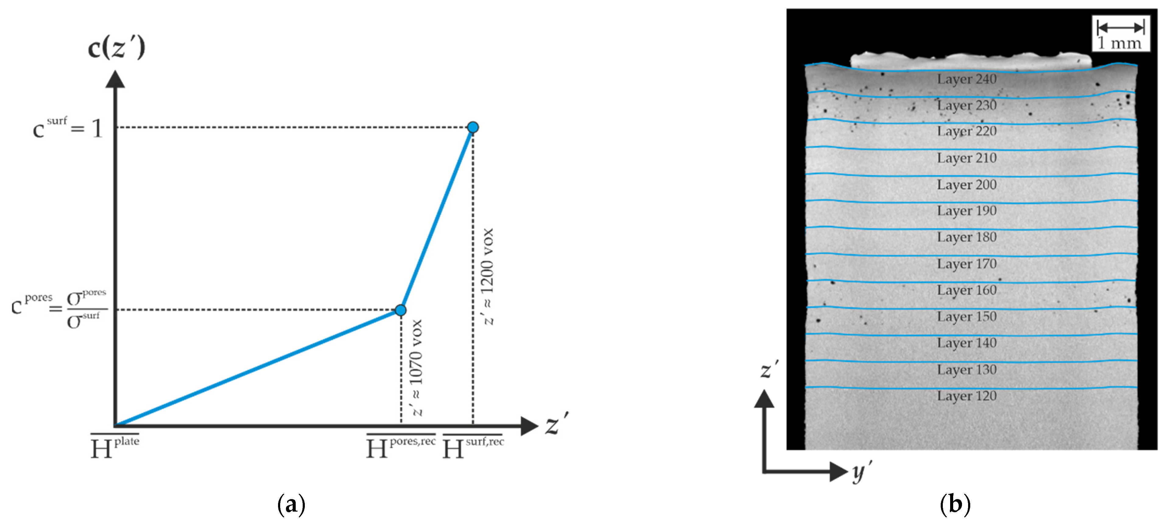
3.2.3. Estimation of the Surface Deformation History

The distribution of the pores in the transition zones between sections of standard VED followed by sections of increased VED was the basis for the estimation of the former surface deformation history. Such pores in the transition zones are called boundary pores hereafter. Due to the increased VED utilized in sections 2, 4, and 6, predominantly keyhole pores were present. Keyhole pores are likely to form at the bottom of the melt pool and be entrapped in its lower part [37]. Inspired by the findings of Ulbricht et al. [7], it is assumed that the topography of the former surface can be reconstructed from the statistically distributed pores at the boundary of the transition zone. The first step to estimate the previous surface deformation was the extraction of the boundary pores. The transition zones from section 1 to 2 and from section 3 to 4 were not regarded due to the low information density resulting from the low number of pores in these sections. The decreased number of pores contributed to the lower increase of VED [38] utilized in these sections (+25% in section 2 and +50% in section 4). Only in the transition from section 5 to 6 was a sufficient number of pores present. A data subset from height z′ = 1050 to 1090 vox (equal to a specimen height of 10.5 μm to 10.9 μm) that contained the lowest boundary pores was extracted from V^proc,bin. The 3D position of each respective pore centroid in the subset was calculated (MATLAB function “regionprops3”) and stored in a 2D array. The pores located at the rim of the obtained disc-shaped point cloud were extracted (MATLAB function “boundary”). For the surface reconstruction, only the pores of the bottom part of the rim were utilized since they were located in the transition zone. These centroids were denoted as H^pores and were located at an average centroid height of approximately z′ = 1070 voxel. Here, the same interpolation algorithm as used for the top surface [36] was applied to reconstruct the surface shape. This shape was denoted as H^pores,rec. Additional smoothing was added to remove local inhomogeneities. H^pores,rec is depicted in Figure 5c. Good agreement was found between the reconstructions H^pores,rec and H^surf,rec. Furthermore, the standard deviation (STD) σ^pores of the original centroid heights in H^pores,rec was calculated to 33 μm, which is significantly lower than the STD σ^surf of H^surf,rec (95 μm).

3.2.4. Determination of a Deformation Adjustment Function

Based on H^pores,rec, a deformation adjustment function g_x′,y′ (z′) was determined for the compensation of the surface deformation history. As stated above, the method assumed that all surface deformations during the manufacturing had an approximately similar shape like the surface deformation H^surf,rec determined in Section 3.2.2. However, the comparison of σ^pore and σ^surf implied that the average height amplitude of the deformed surfaces increased with growing z′. This was taken into account by the introduction of a compression factor c. The idea behind c was the adaption of the average height amplitude in dependency to z′. Due to the given pore distribution, only three reference surfaces were available for the calculation of c: (i) The non-deformed milled surface of the dummy base volume H^plate at z′ = 0 vox with σ^plate = 0, (ii) the surface reconstruction H^pores,rec from the boundary pores at an average height of z′ ≈ 1070 voxel with σ^pores = 33 μm, and (iii) the surface reconstruction H^surf,rec with σ^surf = 95 μm of the specimen top. Due to this lack of information, only a sectional linear interpolation approach was feasible for the calculation of c (see Figure 6a).

The compression factor c is given by:

$$\mathrm{c}\left(z^{\prime }\right)=\{\begin{array}{c}\frac{{\mathrm{m}}_1{z}^{\prime }+{\mathrm{b}}_1}{{\mathsf{\sigma }}^{\mathrm{surf}}}:\overline{{\mathbf{H}}^{\mathrm{plate}}}<z^{\prime }<\overline{{\mathrm{H}}^{\mathrm{pores},\mathrm{rec}}}\\ \frac{{\mathrm{m}}_2{z}^{\prime }+{\mathrm{b}}_2}{{\mathsf{\sigma }}^{\mathrm{surf}}}:\overline{{\mathbf{H}}^{\mathrm{pores},\mathrm{rec}}}\le z^{\prime }<\overline{{\mathbf{H}}^{\mathrm{surf},\mathrm{rec}}}\end{array}$$

(7)

m₁ = 3.902 × 10⁻³, m₂ = 4.479 × 10⁻³ correspond to the slope and b₁ = 0, b₂ = −4.33 correspond to the intercept of g_x′,y′(z′) in the respective interpolation section (see Figure 6a). The sections were chosen corresponding to the average height of the substrate plate $\overline{{\mathbf{H}}^{\mathrm{plate}}}$ = 0, the average height of the extracted pore centroids $\overline{{\mathbf{H}}^{\mathrm{pores},\mathrm{rec}}}$ and the average surface height $\overline{{\mathbf{H}}^{\mathrm{surf},\mathrm{rec}}}$. To obtain values between 0 and 1, a normalization with σ^surf was performed.

The local height deviation at an arbitrary voxel position resulting from the surface deformation was calculated by the deformation adjustment function g_x′,y′(z′):

$${\mathrm{g}}_{x^{\prime },y^{\prime }}\left(z^{\prime }\right)={\mathsf{\Delta }\mathbf{H}}_{x^{\prime },y^{\prime }}^{\mathrm{surf},\mathrm{rec}}·{\mathrm{c}\left(z^{\prime }\right)}_{}$$

(8)

$${\mathsf{\Delta }\mathbf{H}}_{x^{\prime },y^{\prime }}^{\mathrm{surf}}{=\mathbf{H}}_{x^{\prime },y^{\prime }}^{\mathrm{surf},\mathrm{rec}}-\overline{{\mathbf{H}}^{\mathrm{surf},\mathrm{rec}}}$$

(9)

Here, the local height deviation at voxel position x′ and y′ is given by ${\mathsf{\Delta }\mathrm{H}}_{x^{\prime },y^{\prime }}^{\mathrm{surf},\mathrm{rec}}$. Exemplary values of g_x′,y′(z′) for chosen layer heights are depicted in Figure 6b.

3.2.5. Volume Reconstruction Utilizing the Deformation Adjustment Function

Equation (8) gives an incremental floating number which corresponds to the height deviation of the considered voxel with the height z′. The volume reconstruction was performed by the generation of a new volume V^final from the distorted volume V^proc,bin. Here, for each new voxel in V^final, the position of a corresponding voxel in V^proc,bin was calculated and its associated binary value was assigned to the new voxel:

$${\mathbf{V}}^{\mathrm{rec}}(x^{\prime },y^{\prime },z^{\prime }) = {\mathbf{V}}^{\mathrm{proc},\mathrm{bin}}(x^{\prime },y^{\prime },z^{*})$$

(10)

$$\mathrm{with}z* = \lceil z^{\prime }+{\mathrm{g}}_{x^{\prime },y^{\prime }}\left(z^{\prime }\right)\rfloor$$

(11)

z* was rounded to avoid non-integer values. Since the specimen height was locally adjusted to the CAD height, the number of voxels containing density information was larger in V^final than in V^proc,bin. Therefore, single voxel values from V^proc,bin were duplicated during the assignment to V^final. The decision to duplicate a voxel was determined by the rounding operation of z*. The maximum percentage of duplicated voxel at a single x′-y′ position was approximated to ~3% from the maximum height difference between the real specimen and the CAD (~400 μm). The final size of V^final was 711 × 711 × 1200 voxels. For evaluation, the adjusted top surface of V^final was extracted by the thresholding algorithm described Section 3.2.2 (Figure 5d). After the removal of the cross and the label landmark (see Section 3.2.2), the STD of the surface height of V^final was calculated to 30 μm. This is a significant decrease compared to the surface of V^proc (STD of 95 μm). Furthermore, a comparison of the pore distribution in the transition zone pre- and post-adjustment is depicted in Figure 7. In the hypothetical case of a specimen free of surface deformations, the pores were expected to appear at an approximately similar height z′ in the specimen under the assumption of a comparatively small statistical depth variation of keyhole pores. The former dataset is distinguished by pores being distributed heterogeneously, appearing at first especially in the right half of the specimen in Figure 7a with a transition to the left half with growing z′. The height difference between the first appearance of keyhole pores in the cylinder right half to a pore distribution over the entire specimen cross-section amounts to approximately 10 to 11 voxels. In the case of the adjusted dataset, this height difference is decreased to approximately 5 to 6 voxels, especially when disregarding the pores present at the specimen rim. These were presumably LoF voids resulting from the interface between bulk and contour scans [7,39,40,41]. Furthermore, the described transition in the former dataset from right specimen half to left specimen half is no longer present here.

Due to the performed surface adjustment, the utilization of a simple 3D image-by-image registration algorithm was enabled.

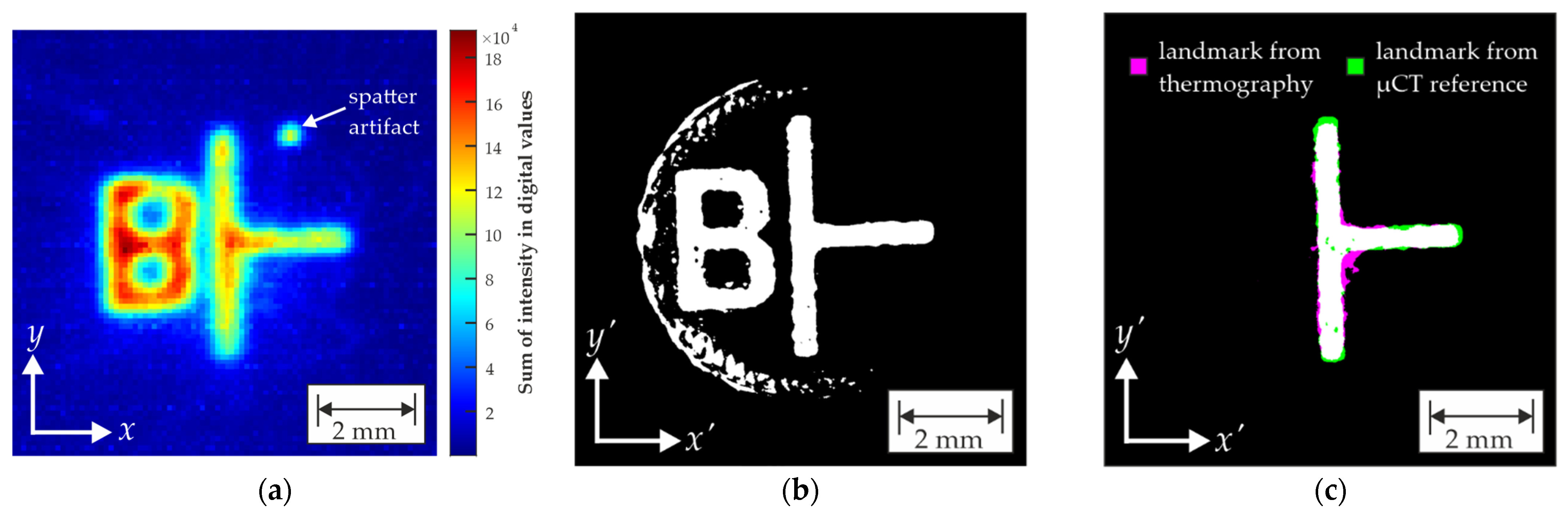
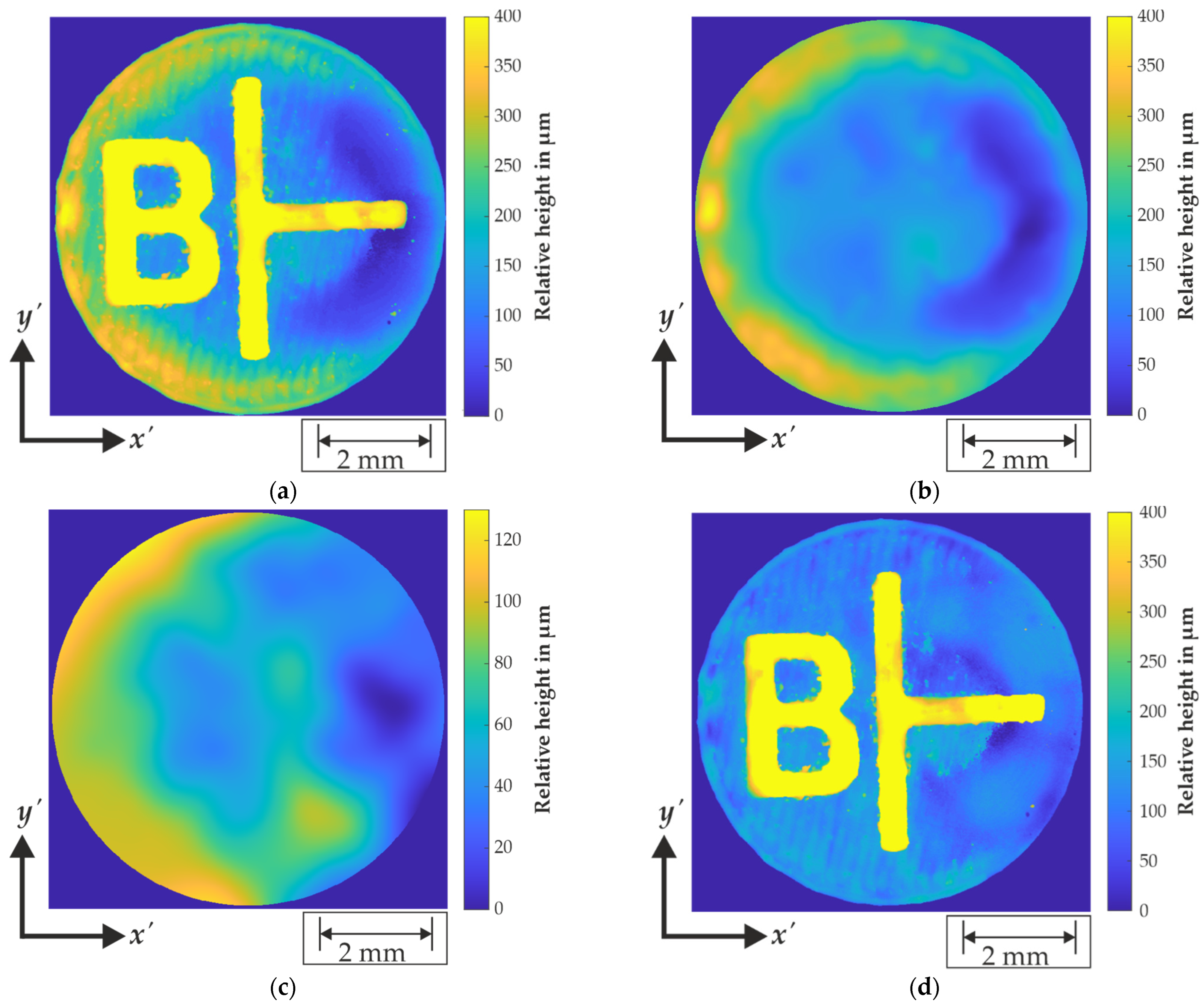
3.3. Image Registration

The spatial image registration was performed using the MATLAB Registration Estimator Toolbox. Here, several different feature-based and intensity-based algorithms for image registration are available. For this study, a monomodal intensity-based algorithm [10] was chosen because the datasets were acquired by different imaging techniques and therefore, had different spatial resolutions and different geometric features. The thermograms were labeled as moving images which were spatially transformed to be registered on the XCT fixed images [11]. A registration function T was generated using images of the cross landmark on the specimen top surface. The cross landmark was visible in both thermography and XCT image data (see Figure 8). In the case of the XCT data, the cross was extracted from the cross-section slice of V^final. Regarding the thermogram data, the extraction of the cross landmark was performed from a sum of intensity image from the thermograms of the landmark manufacturing. Here, the pixel temperatures of all 2D thermograms from the manufacturing series of specimen layer were summed up and normalized afterwards. Layer 242 was chosen for the sum of intensity image since the landmark structures were the most clearly identifiable here. Both images were further processed to improve the clearness of the landmark geometry. At first, noisy background elements were removed from the image using arithmetical image multiplication and a polygonal mask. The low spatial resolution of the thermographic camera demanded the use of morphological and median filters to clarify the cross edges. Furthermore, the introduced preprocessing in Section 3.1 was applied on the thermography cross landmark image. Finally, the image was binarized using a global threshold.

Four different transformation models (“similarity”, “affine”, “rigid”, and “translation”) were available in the MATLAB toolbox for the monomodal registration to produce a registration function. These models exhibit different degrees of freedom concerning the available transformations. The highest degree of freedom is given by the similarity model that allows translation, rotation, shearing, and scaling of the moving image. The affine model does not allow shearing, while only translation and rotation are available when using the rigid model. In the case of the translation model, only image translation is applied on the moving image. Due to the performed resampling and rectification from the preprocessing of the cross landmark, the moving image already had the same image scale as the XCT image and present distortions were adjusted. Furthermore, the size of the sum of intensity image of the cross landmark in the thermogram dataset may be artificially enlarged by thermal expansion and the choice of the binarization threshold. Therefore, shearing and scaling are unnecessary degrees of freedom that might introduce registration inaccuracy. Two registration functions based on the rigid and the translation model were determined. In the following, the obtained registration functions were applied on the slices of the preprocessed thermogram datasets A^k and the preprocessed XCT dataset V^final [34]:

$$\mathrm{T}({\mathrm{A}}_z^{\mathrm{k},2\mathrm{D}})\leftrightarrow {\mathrm{V}}_{z^{\prime }}^{\mathrm{final},2\mathrm{D}}\mathrm{with}z=z^{\prime }$$

(12)

Here, ${\mathrm{A}}_z^{\mathrm{k},2\mathrm{D}}$ correspond to a 2D x-y slice of A^k and ${\mathrm{V}}_{z\prime }^{\mathrm{final},2\mathrm{D}}$ to the 2D x′-y′ slice of V^final. As stated in Section 1, the evaluation of the registration accuracy is often challenging. In this study, a simple method was utilized to evaluate the registration results. A full dataset of layer maps from thermography (chosen feature: melt pool area) was registered with the corresponding XCT dataset. Afterwards, the contours of the registered x-y slices were approximated by a circle fit [32]. In the case of the thermogram dataset, a binarization using a manually chosen threshold was necessary for the detection of the boundary edges. From the circle fit, the average distance ΔD between the circle centroids of the registered datasets was calculated for all slices:

$$\mathsf{\Delta }\mathrm{D}=\frac{1}{{\mathrm{n}}_{\mathrm{slice}}}{\displaystyle \sum }_{\mathrm{i}=1}^{n_{\mathrm{slice}}}\sqrt{{\left(x_z^{\mathrm{cen}} {-x^{\prime }}_{z^{\prime }}^{\mathrm{cen}}\right)}^2+{\left(y_z^{\mathrm{cen}} {-y^{\prime }}_{z^{\prime }}^{\mathrm{cen}}\right)}^2}{\mathrm{with}z=z^{\prime }}_{}$$

(13)

Here, the centroid position of the thermogram feature image is given by $x_z^{\mathrm{cen}}$ and $y_z^{\mathrm{cen}}$, while the centroid position of the XCT image is given by ${x^{\prime }}_{z^{\prime }}^{\mathrm{cen}}$ and ${y^{\prime }}_{z^{\prime }}^{\mathrm{cen}}$. $\mathsf{\Delta }\mathrm{D}$ was an indicator for the translation error that was present after the registration. Furthermore, the MAE of average difference of the circle radius $\mathsf{\Delta }R$was calculated as a measure of the scaling error. The results are shown in

Table 4. Geometric errors resulting from different transformation modes of registration in the corresponding sections. Here, ΔD corresponds to the MAE of the distance between the circle fit centroids and ΔR to the MAE of the difference between the circle fit radii. The STD of both sizes is given by σ_ΔD and σ_ΔR, respectively.

Transformation Model (Including Degrees of Freedom)	Section	ΔD in μm	σΔD in μm	ΔR in μm	σΔR in μm
Rigid (translation and rotation)	1	23	±12	21	±8
	2	42	±20	38	±6
	3	23	±11	25	±7
	4	65	±29	59	±11
	5	25	±12	30	±11
	6	80	±31	57	±23
Translation (translation)	1	27	±13	19	±8
	2	43	±19	37	±5
	3	29	±12	23	±7
	4	53	±22	55	±9
	5	27	±12	28	±10
	6	64	±27	55	±23

.

4. Discussion

It is important to place this investigation in the overall context of irregularity prediction in L-PBF parts. The precise prediction of irregularities based on the obtained thermographic in situ monitoring data was the objective. The registration is a necessary step to align monitoring and reference datasets. Therefore, the achieved registration precision is a crucial information because it limits the effective volume size in which irregularities can be accurately predicted.

The preprocessing of the thermogram data included, in the case of melt pool-based features, an interpolation from a sparse point cloud of voxels to a resampled 3D volume dataset. This was performed to adjust the thermogram voxel sizes to the XCT voxel size. Thus, the datasets could be registered more precisely with a theoretical accuracy lower than the pixel resolution of the IR camera, 100 μm². Single voxel values of the interpolated datasets should be treated with care because it is uncertain if they necessarily reflect the exact thermal history of the temporally high dynamic L-PBF process. It can be concluded that the temporal and spatial resolution of the raw thermograms is important information that should be considered for the prediction of irregularities. Especially if the original thermogram datasets have a lower spatial information density than the registered datasets, a further resampling of the registered datasets to a larger voxel size might be necessary.

In the context of XCT data preprocessing, it was found that an adjustment of the detected surface deformation is of vital importance for the overall registration accuracy. The obtained results from the introduced adjustment method are promising since they show a clear decrease in shape deformation (compare Figure 5d and Figure 7). Nonetheless, it is necessary to critically analyze the single XCT preprocessing steps that were performed.

The basic method of reconstructing former surface deformations from the internal void distribution in the part was strongly motivated by the findings of Ulbricht et al. [7] and their observations related to the surface deformation. Here, multiple indications of the former surface deformations were visible in the XCT data due to the implementation of artificial notches in their design. In the specimen investigated in the current study, no such notches were present since their implementation might have interfered with the presence of keyhole pores whose formation was forced by the chosen design. Therefore, the available information for surface reconstruction was limited. Only pores in one section could be used for the reconstruction of the surface deformation history. From this lack of information arose the decision to utilize a linear sectional approach for the calculation of the compression factor c. This choice might be an oversimplification in terms of describing the surface deformation history. The potential need of more complex fitting approaches such as higher order polynomials or exponential functions to describe the surface deformation history will be investigated in future research. In future experimental designs, the insertion of artificial voids as references instead of boundary pores could be used for an easier determination of the deformation history.

The chosen simple fitting approach for the compression factor c well compensated the error induced by the surface deformation (Figure 5d and Figure 7). The results show that the specimen deformation was determined accurately by the chosen customized thresholding and surface reconstruction algorithm. Here, the choice of other registration landmarks which are not positioned on the specimen top could improve this result even further, since the step of surface reconstruction of missing areas would be omitted.

In order to describe the surface deformation history, the assumption was made that all surface deformations during manufacturing had an approximately similar shape to the deformation of the specimen top. The results indicate that this assumption is promising. The deformation reconstructed from the pore centroids at an approximate specimen height of z′ = 1070 voxel is in good agreement with the determined top surface deformation. This is remarkable since the reconstruction is based on the positional information of the present keyhole pores.

The formation of keyhole pores is connected to unstable conditions in the melt pool keyhole [37]. As a result, keyhole pores can occur spatially irregularly during the manufacturing of a scan track (compare Figure 7). Additionally, the melt pool depth varies to a certain extent. As a result, the z′ position of pores which result from a single layer manufacturing can fluctuate. The melt pool depth was shown to depend on the laser processing parameters. Mohr et al. [25] found melt pool depths of 213 ± 19 μm for a VED of 65.5 J/mm³ and 471 ± 54 μm for a VED of 152.7 J/mm³ using the same machine and material that was utilized in the present study. It can be assumed that the average melt pool depths from the VED utilized in section 6 (114.45 J/mm³) lay in between these results. However, regarding the pores that were utilized for the former surface deformation reconstruction, the positional fluctuations are limited by the manufacturing of overlying layers. Here, the keyhole of the new layer can interact with the lower pores which may lead to the escape of the entrapped gas or a recombination with new pores. Therefore, the positional fluctuation is effectively limited to the layer thickness (50 μm).

The heterogeneous spatial pore distribution and the fluctuation in the vertical pore location were identified as interfering factors for the reconstruction of the former surface deformation. Nonetheless, the surface deformation calculated by pore distribution (Figure 5c) showed similar shape tendencies as the top surface deformation (Figure 5a). From that, it can be concluded that the history of surface deformation is effectively linked to the resulting pore location. Precise knowledge of the surface deformation history is, therefore, essential for an allocation of in situ sensor data to the porosity information obtained from XCT. To the best of the authors’ knowledge, these findings are new and underline the importance of shape adjustment in the registration procedure for irregularity prediction.

It needs to be remarked that the density information of the manufactured specimen is effectively locally distorted by the shape adjustment to match with the “ideal” specimen geometry given by the CAD. Therefore, the quantitative void sizes in the adjusted dataset should be analyzed with care since they might differ from the results in the raw dataset. However, a quantitative void analysis can be enabled again if the applied deformation adjustment is reverted.

In terms of the image registration, the allowed transformation options of the investigated registration models were rotation and translation. Due to the performed preprocessing of both datasets, it was decided that shearing and scaling as additional transformations were unnecessary degrees of freedom. The results (Table 4) show that the lowest errors were achieved when applying the rigid model in section 3. In the section of increased VED, lower accuracy was achieved. This was presumably caused by the lateral shrinkage present in these sections (visible in Figure 4 and Figure 6b). The shrinkage seemed to prevent the algorithm to produce even better results. The comparison between the registration functions showed that the translation model performed better in the section of increased VED. The additionally allowed rotation of the rigid model appears to be counterproductive here and the results indicate that both XCT and thermography datasets were already aligned well from preprocessing. The lower performance from the rigid transformation might result from the shape deviations between the cross landmark images that might have induced an unnecessary rotation.

The results show that already a simple transformation function with a low number of degrees of freedom is sufficient for the registration of the preprocessed datasets. For data that are not preprocessed, it might be a reasonable choice to choose a model that contains shearing and scaling. Here, the quality of the geometric landmark is a crucial factor. Furthermore, the results show the potential of the developed registration method if no lateral shrinkage is present. An extension of the algorithm to improve the registration accuracy if lateral shrinkage is present will be the objective of future studies.

5. Conclusions

In this study, a 3D image-to-image registration was performed on datasets of thermal features extracted from in situ thermography and a corresponding XCT dataset. The registration was performed as a prerequisite for irregularity prediction. Extensive data preprocessing was conducted to obtain similar data dimensionalities to enable the utilization of the chosen, simple registration method. The preprocessing of the thermal feature dataset included the compensation of image distortion, the interpolation of missing datapoints and a resampling to the voxel scale of the XCT data. In the case of the XCT dataset, vertical shrinkage was preliminary corrected from the height information of a staircase landmark structure. Furthermore, a novel shape adjustment method was introduced to eliminate the surface deformation history that was found in the entire part. An image registration function was derived from the utilization of geometric landmarks located on the specimen top surface. The registration accuracy was assessed among the obtained geometrical errors in the registered datasets. From the results of the performed image registration, the following conclusions are drawn:

• Thermally induced warping and solidification shrinkage, especially in the form of surface deformations, are a major challenge for the image registration because it prevents the application of simple registration methods. In this study, it was demonstrated that the distribution of boundary keyhole pores within the observed specimen can be utilized to reconstruct the surface deformation for a specific point in time within the manufacturing. Furthermore, it was shown that an adjustment function based on the approximated surface deformation history enables the adjustment of the part deformation and the application of a simple 3D image-to-image registration.
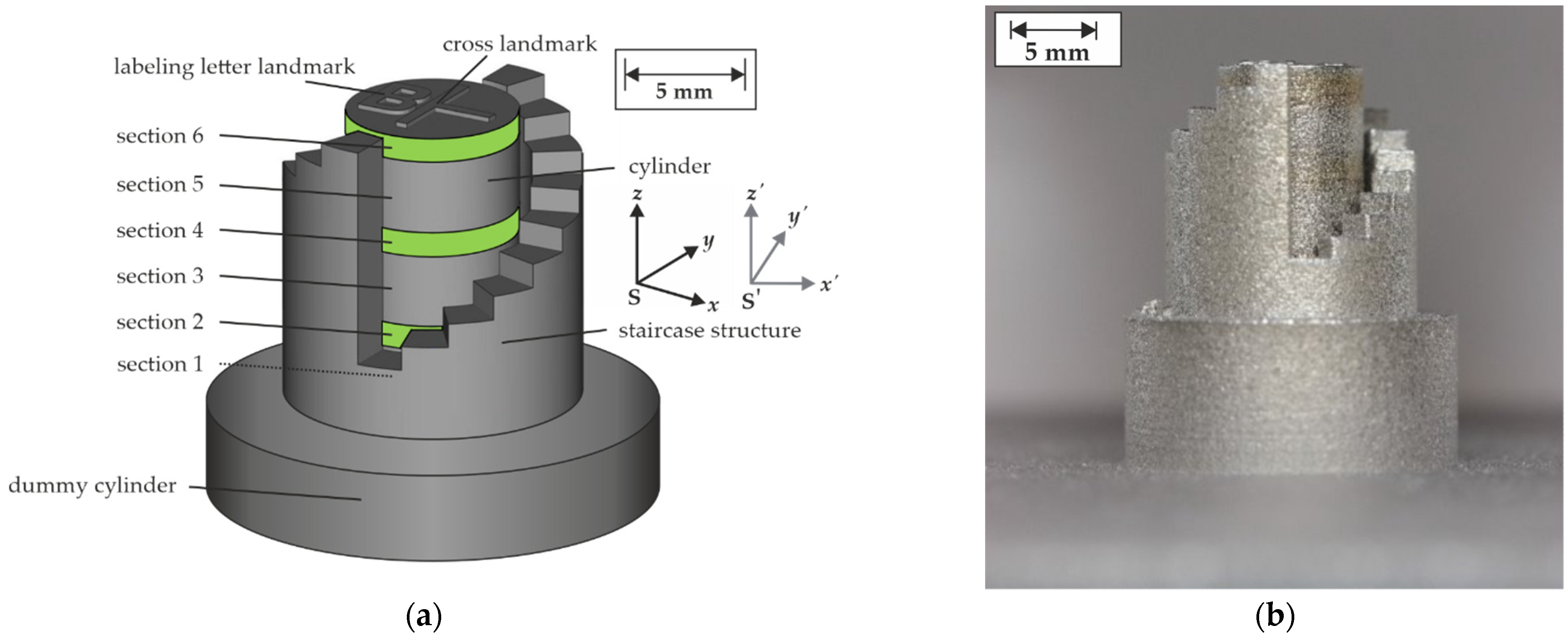
• The geometrical references that were included in the specimen design proved to be very beneficial for the data registration. The surrounding staircase structure provided information for the preliminary adjustment of the vertical part shrinkage. The cross label added on the specimen top could be utilized to generate a registration function. A drawback of this structure was its disruptive influence during the reconstruction of the top surface information.
• The performed registration resulted in a translation error of 23 μm ± 12 μm and a scaling error of 21 μm ± 8 μm (rigid model in section 3). These errors are significantly lower than the spatial resolution achieved by the IR camera. From the utilization of the adjustment function, it was found that high improvement was achieved in comparison to the unadjusted dataset. Based on these findings, it is possible for the first time to consider the registration accuracy in irregularity prediction modeling.

In future studies, the registered datasets will be used to generate a ML-based model for the prediction of irregularities within the produced part. Here, the obtained registration error information will be incorporated to determine the spatial resolution in which the porosity can be reasonably predicted. Apart from that, we aim to improve the algorithm to make it more robust if lateral shrinkage is present in the part. The insertion of artificial voids within the specimen is a promising option to reconstruct the surface information at different specimen heights. A further option in this regard is the in situ measurement of the part surface topography by laser profilometry that can be integrated into the process. By that, a more accurate deformation adjustment can be achieved which will further increase the registration accuracy and ultimately the irregularity prediction accuracy.

References

1. Al Rashid, A.; Khan, S.A.; Al-Ghamdi, S.G.; Koç, M. Additive Manufacturing: Technology, Applications, Markets, and Opportunities for the Built Environment. Autom. Constr. 2020, 118, 103268. [Google Scholar] [CrossRef]
2. Tapia, G.; Elwany, A. A Review on Process Monitoring and Control in Metal-Based Additive Manufacturing. J. Manuf. Sci. Eng. 2014, 136, 060801. [Google Scholar] [CrossRef]
3. Frazier, W.E. Metal Additive Manufacturing: A Review. J. Mater. Eng. Perform. 2014, 23, 1917–1928. [Google Scholar] [CrossRef]
4. Fritsch, T.; Farahbod-Sternahl, L.; Serrano-Muñoz, I.; Léonard, F.; Haberland, C.; Bruno, G. 3d Computed Tomography Quantifies the Dependence of Bulk Porosity, Surface Roughness, and Re-Entrant Features on Build Angle in Additively Manufactured In625 Lattice Struts. Adv. Eng. Mater. 2021, 2021, 2100689. [Google Scholar] [CrossRef]
5. McCann, R.; Obeidi, M.A.; Hughes, C.; McCarthy, É.; Egan, D.S.; Vijayaraghavan, R.K.; Joshi, A.M.; Acinas Garzon, V.; Dowling, D.P.; McNally, P.J.; et al. In-Situ Sensing, Process Monitoring; Machine Control in Laser Powder Bed Fusion: A Review. Addit. Manuf. 2021, 45, 102058. [Google Scholar] [CrossRef]
6. Lough, C.S.; Liu, T.; Wang, X.; Brown, B.; Landers, R.G.; Bristow, D.A.; Drallmeier, J.A.; Kinzel, E.C. Local Prediction of Laser Powder Bed Fusion Porosity by Short-Wave Infrared Imaging Thermal Feature Porosity Probability Maps. J. Mater. Processing Technol. 2022, 302, 117473. [Google Scholar] [CrossRef]
7. Ulbricht, A.; Mohr, G.; Altenburg, S.J.; Oster, S.; Maierhofer, C.; Bruno, G. Can Potential Defects in Lpbf Be Healed from the Laser Exposure of Subsequent Layers? A Quantitative Study. Metals 2021, 11, 1012. [Google Scholar] [CrossRef]
8. Grasso, M.; Remani, A.; Dickins, A.; Colosimo, B.M.; Leach, R.K. In-Situ Measurement and Monitoring Methods for Metal Powder Bed Fusion: An Updated Review. Meas. Sci. Technol. 2021, 32, 112001. [Google Scholar] [CrossRef]
9. Oliveira, F.P.; Tavares, J.M. Medical Image Registration: A Review. Comput. Methods Biomech. Biomed. Eng. 2014, 17, 73–93. [Google Scholar] [CrossRef]
10. Gao, Z.; Gu, B.; Lin, J. Monomodal Image Registration Using Mutual Information Based Methods. Image Vis. Comput. 2008, 26, 164–173. [Google Scholar] [CrossRef]
11. Klein, S.; Staring, M.; Murphy, K.; Viergever, M.A.; Pluim, J.P. Elastix: A Toolbox for Intensity-Based Medical Image Registration. IEEE Trans. Med. Imaging 2010, 29, 196–205. [Google Scholar] [CrossRef] [PubMed]
12. Alpert, N.M.; Berdichevsky, D.; Levin, Z.; Morris, E.D.; Fischman, A.J. Improved Methods for Image Registration. Neuroimage 1996, 3, 10–18. [Google Scholar] [CrossRef] [PubMed] [Green Version]
13. Guo, W.G.; Tian, Q.; Guo, S.; Guo, Y. A Physics-Driven Deep Learning Model for Process-Porosity Causal Relationship and Porosity Prediction with Interpretability in Laser Metal Deposition. CIRP Ann. 2020, 69, 205–208. [Google Scholar] [CrossRef]
14. Sinclair, L.; Leung, C.L.A.; Marussi, S.; Clark, S.J.; Chen, Y.; Olbinado, M.P.; Rack, A.; Gardy, J.; Baxter, G.J.; Lee, P.D. In Situ Radiographic and Ex Situ Tomographic Analysis of Pore Interactions During Multilayer Builds in Laser Powder Bed Fusion. Addit. Manuf. 2020, 36, 101512. [Google Scholar] [CrossRef]
15. Mohr, G.; Nowakowski, S.; Altenburg, S.J.; Maierhofer, C.; Hilgenberg, K. Experimental Determination of the Emissivity of Powder Layers and Bulk Material in Laser Powder Bed Fusion Using Infrared Thermography and Thermocouples. Metals 2020, 10, 1546. [Google Scholar] [CrossRef]
16. Feldkamp, L.A.; Davis, L.C.; Kress, J.W. Practical Cone-Beam Algorithm. J. Opt. Soc. Am. A 1984, 1, 612–619. [Google Scholar] [CrossRef] [Green Version]
17. Schörner, K.; Goldammer, M.; Stephan, J. Scatter Correction by Modulation of Primary Radiation in Industrial X-Ray Ct: Beam-Hardening Effects and Their Correction. In Proceedings of the International Symposium on Digital Industrial Radiology and Computed Tomography—Mo.3.2, Berlin, Germany, 20–22 June 2011. [Google Scholar]
18. Ametova, E.; Ferrucci, M.; Dewulf, W. A Tool for Reducing Cone-Beam Artifacts in Computed Tomography Data. In Proceedings of the 7th Conference on Industrial Computed Tomography (iCT 2017), Leuven, Belgium, 7–9 February 2017. [Google Scholar]
19. Roche, R.C.; Abel, R.A.; Johnson, K.G.; Perry, C.T. Quantification of Porosity in Acropora Pulchra (Brook 1891) Using X-ray Micro-Computed Tomography Techniques. J. Exp. Mar. Biol. Ecol. 2010, 396, 1–9. [Google Scholar] [CrossRef]
20. Shah, P.; Racasan, R.; Bills, P. Comparison of Different Additive Manufacturing Methods Using Computed Tomography. Case Stud. Nondestruct. Test. Eval. 2016, 6, 69–78. [Google Scholar] [CrossRef] [Green Version]
21. Mireles, J.; Ridwan, S.; Morton, P.A.; Hinojos, A.; Wicker, R.B. Analysis and Correction of Defects within Parts Fabricated Using Powder Bed Fusion Technology. Surf. Topogr. Metrol. Prop. 2015, 3, 034002. [Google Scholar] [CrossRef]
22. Lough, C.S.; Wang, X.; Smith, C.C.; Landers, R.G.; Bristow, D.A.; Drallmeier, J.A.; Brown, B.; Kinzel, E.C. Correlation of Swir Imaging with Lpbf 304l Stainless Steel Part Properties. Addit. Manuf. 2020, 35, 101359. [Google Scholar] [CrossRef]
23. Coeck, S.; Bisht, M.; Plas, J.; Verbist, F. Prediction of Lack of Fusion Porosity in Selective Laser Melting Based on Melt Pool Monitoring Data. Addit. Manuf. 2019, 25, 347–356. [Google Scholar] [CrossRef]
24. Forien, J.-B.; Calta, N.P.; DePond, P.J.; Guss, G.M.; Roehling, T.T.; Matthews, M.J. Detecting Keyhole Pore Defects and Monitoring Process Signatures During Laser Powder Bed Fusion: A Correlation between in Situ Pyrometry and Ex Situ X-ray Radiography. Addit. Manuf. 2020, 35, 101336. [Google Scholar] [CrossRef]
25. Mohr, G.; Altenburg, S.J.; Ulbricht, A.; Heinrich, P.; Baum, D.; Maierhofer, C.; Hilgenberg, K. In-Situ Defect Detection in Laser Powder Bed Fusion by Using Thermography and Optical Tomography—Comparison to Computed Tomography. Metals 2020, 10, 103. [Google Scholar] [CrossRef] [Green Version]
26. Taherkhani, K.; Sheydaeian, E.; Eischer, C.; Otto, M.; Toyserkani, E. Development of a Defect-Detection Platform Using Photodiode Signals Collected from the Melt Pool of Laser Powder-Bed Fusion. Addit. Manuf. 2021, 46, 102152. [Google Scholar] [CrossRef]
27. Gobert, C.; Reutzel, E.W.; Petrich, J.; Nassar, A.R.; Phoha, S. Application of Supervised Machine Learning for Defect Detection During Metallic Powder Bed Fusion Additive Manufacturing Using High Resolution Imaging. Addit. Manuf. 2018, 21, 517–528. [Google Scholar] [CrossRef]
28. Oster, S.; Maierhofer, C.; Mohr, G.; Hilgenberg, K.; Ulbricht, A.; Altenburg, S.J. Investigation of the Thermal History of L-Pbf Metal Parts by Feature Extraction from in-Situ Swir Thermography. In Proceedings of the Thermosense: Thermal Infrared Applications XLIII, online, 12–16 April 2021; p. 117430C. [Google Scholar] [CrossRef]
29. Scheuschner, N.; Strasse, A.; Altenburg, S.J.; Gumenyuk, A.; Maierhofer, C. In-Situ Thermographic Monitoring of the Laser Metal Deposition Process. In Proceedings of the II International Conference on Simulation for Additive Manufacturing, Pavia, Italy, 11–13 September 2019. [Google Scholar]
30. Herman, G.T. Correction for Beam Hardening in Computed Tomography. Phys. Med. Biol. 1997, 24, 81–106. [Google Scholar] [CrossRef]
31. Schindelin, J.; Arganda-Carreras, I.; Frise, E.; Kaynig, V.; Longair, M.; Pietzsch, T.; Preibisch, S.; Rueden, C.; Saalfeld, S.; Schmid, B.; et al. Fiji: An Open-Source Platform for Biological-Image Analysis. Nat. Methods 2012, 9, 676–682. [Google Scholar] [CrossRef] [Green Version]
32. Chernov, N. Circle Fit (Pratt Method). Available online: https://www.mathworks.com/matlabcentral/fileexchange/22643-circle-fit-pratt-method (accessed on 1 November 2021).
33. Phansalkar, N.; More, S.; Sabale, A.; Madhuri, J. Adaptive Local Thresholding for Detection of Nuclei in Diversity Stained Cytology Images. In Proceedings of the 2011 International Conference on Communications and Signal Processing, Kerala, India, 10–12 February 2011. [Google Scholar] [CrossRef]
34. Markelj, P.; Tomazevic, D.; Likar, B.; Pernus, F. A Review of 3d/2d Registration Methods for Image-Guided Interventions. Med. Image Anal. 2012, 16, 642–661. [Google Scholar] [CrossRef]
35. Kiekens, K.; Welkenhuyzen, F.; Tan, Y.; Bleys, P.; Voet, A.; Kruth, J.P.; Dewulf, W. A Test Object with Parallel Grooves for Calibration and Accuracy Assessment of Industrial Computed Tomography (Ct) Metrology. Meas. Sci. Technol. 2011, 22, 115502. [Google Scholar] [CrossRef]
36. D’Errico, J. Surface Fitting Using Gridfit. Available online: https://www.mathworks.com/matlabcentral/fileexchange/8998-surface-fitting-using-gridfit (accessed on 5 July 2021).
37. Hojjatzadeh, S.M.H.; Parab, N.D.; Guo, Q.; Qu, M.; Xiong, L.; Zhao, C.; Escano, L.I.; Fezzaa, K.; Everhart, W.; Sun, T.; et al. Direct Observation of Pore Formation Mechanisms During Lpbf Additive Manufacturing Process and High Energy Density Laser Welding. Int. J. Mach. Tools Manuf. 2020, 153, 103555. [Google Scholar] [CrossRef]
38. Wang, L.; Zhang, Y.; Chia, H.Y.; Yan, W. Mechanism of Keyhole Pore Formation in Metal Additive Manufacturing. Npj Comput. Mater. 2022, 8, 22. [Google Scholar] [CrossRef]
39. Ertay, D.S.; Ma, H.; Vlasea, M. Correlative Beam Path; Pore Defect Space Analysis for Modulated Powder Bed Laser Fusion Process. In Proceedings of the 2018 International Solid Freeform Fabrication Symposium, Austin, TX, USA, 13–15 August 2018. [Google Scholar] [CrossRef]
40. Du Plessis, A. Effects of Process Parameters on Porosity in Laser Powder Bed Fusion Revealed by X-ray Tomography. Addit. Manuf. 2019, 30, 100871. [Google Scholar] [CrossRef]
41. Jost, E.W.; Miers, J.C.; Robbins, A.; Moore, D.G.; Saldana, C. Effects of Spatial Energy Distribution-Induced Porosity on Mechanical Properties of Laser Powder Bed Fusion 316l Stainless Steel. Addit. Manuf. 2021, 39, 101875. [Google Scholar] [CrossRef]
Figure 1. (a) Specimen design including staircase structure, top surface cross landmark, labeling letter landmark, dummy cylinder, and the introduced coordinate systems S and S′. The green areas mark sections that were manufactured using increased VED. In this view, section 1 is hidden behind the staircase which is indicated by the dashed line. (b) Manufactured specimen on dummy cylinder. Adapted from Ref. [28].
Metals 12 00947 g001
Figure 2. Schematic overview the processing steps for the registration of thermographic and XCT datasets. The dashed lines indicate which steps correspond to the data preprocessing and which correspond to the registration. Datasets are indicated by bold frames.
Metals 12 00947 g002
Figure 3. Preprocessing of thermogram feature data (here: melt pool blob size) of layer 59. (a) Incremental data points of melt pool blob size containing image distortion. (b) Rectified and resampled thermogram with an adjusted scale of 10 μm/pix.
Metals 12 00947 g003
Figure 4. Cross-sectional slice of XCT reference volume at a depth of x′ = 3 mm. Gray value variations in the bulk material are image artifacts originated by the cone-beam reconstruction of strong absorbing material. Height elevations on the surface rim and lateral shrinkage in the section of increased VED are visible. The approximated top surface shape (continuous blue line) is repeated below (dashed blue line) for a better comparison with the pore distribution. In Detail A, the areas of local surface height increase close to the landmarks are marked by blue circles.
Metals 12 00947 g004
Figure 5. (a) Part surface extracted by thresholding algorithm. (b) Reconstructed part surface after removal of registration landmarks. (c) Reconstructed surface from lowest pores in the transition zone (between sections 5 and 6) at an approximately average specimen height of 10.7 mm. (d) Part surface after application of deformation adjustment function extracted by thresholding algorithm.
Metals 12 00947 g005
Figure 6. (a) Qualitative illustration of the linear sectional fit for the determination of the compression factor c. (b) Cross-sectional slice of the XCT data at a depth of 3.5 mm. The height deviations corresponding to the manufacturing layers calculated from gx′,y′(z′) are depicted as blue lines.
Metals 12 00947 g006
Figure 7. Pore distribution between section 5 and 6 starting at a specimen height of approximately 1050 voxels (10.5 mm) increasing by z′ = 1 voxel (10 μm) per image slice (a) before deformation adjustment (Vproc,bin) and (b) after deformation adjustment (Vfinal). While the pore appearance in (a) is mainly starting on the right specimen half and transitions over the course of 10 image slices to the left half, the pore appearance in (b) begins mainly in the center and transitions faster (approximately in 5 image slices) from singular pores to a widespread distribution over the entire cross-section. The dashed red lines indicate the approximate starting and stopping points of the pore transition and are added to increase the readability of the figure. The starting points were manually approximated based on the appearance of a sufficient number of clearly identifiable pores in the cylinder bulk. The stopping points were manually approximated as the images in which pores appeared in major parts of the bulk.
Metals 12 00947 g007
Figure 8. (a) Sum of temperature image from the raw 4D thermogram dataset. (b) x′-y′ slice of Vbin at a height of z′ = 1205 vox. (c) Extracted and processed cross labels from (a,b) after the spatial registration was performed. Shown here is a monomodal translation registration with a quality of 0.958 calculated by the MATLAB Registration Estimator Toolbox. White areas correspond to overlapping area, while pink and green correspond to deviating areas.
Metals 12 00947 g008