Research on Thickness Defect Control of Strip Head Based on GA-BP Rolling Force Preset Model

Abstract

Due to the inaccuracy of the preset rolling force of cold rolling, there is a severe thickness defect in the strip head after cold rolling due to the flying gauge change (FGC), which affects the yield of the strip. This paper establishes a rolling force preset model (RFPM) by combining the rolling force optimization model (RFOM) and the rolling force deviation prediction model (RFDPM). The RFOM used a genetic algorithm (GA) to optimize the deformation resistance and friction coefficient models. The RFDPM is constructed using a backpropagation (BP) neural network. The calculation result of the RFPM shows that the average fraction defect of the preset rolling force is only 1.24%, which proves that the RFPM has good calculation accuracy. Experiments show that the defect length proportion of the strip head thickness at less than 20 m after FGC increases from 38.8% to 55.8%, while the average defect length decreases from 47.3 m to 29.6 m, effectively improving the yield of cold rolling.

1. Introduction

Improving the yield of cold rolling strips on the premise of ensuring product quality is the constant pursuit of enterprises [1,2]. FGC technology can produce strips with different widths, thicknesses, or yield strengths (YS) and achieve endless rolling in tandem cold rolling mills (TCM) [3]. If the rolling force that is set during the dynamic specification change is inaccurate, it is easy to cause thickness fluctuation in the next strip head. Therefore, improving the accuracy of the rolling force setting value is very important for improving the yield [4,5].

The rolling force model is one of the most important models in steel rolling. Many scholars use methods such as theoretical models, finite element simulations, optimization algorithms, or artificial neural networks to improve the accuracy of the rolling force model. Theoretical models are widely used because they can clearly show the physical relationships between the parameters. Zhang et al. [6] proposed a new tangent velocity model and corresponding strain rate fields to accurately predict the rolling force in the hot-strip rolling process; by minimizing the total power function, an analytical solution of the rolling force was obtained. You et al. [7] proposed a rolling force model of the arc-tangent velocity field using the upper bound method. The model is based on the virtual work principle and maximum plastic work principle, and the accuracy of the model is verified by the finite element method. Peng et al. [8] proposed a method to predict the rolling force of cold rolling, based on plastic mechanics. The analysis and solution of the rolling torque, rolling force, and stress state coefficient are obtained by minimizing the total power, which includes the internal plastic power, frictional power, shear power, and tension power. Finally, the validity of the model was proven through an industry experiment. Confusingly, the accuracy of their new model was not significantly better than HIll’s model, and the proportion in which the actual rolling force deviations were within 5% was only 77.2%. Liu et al. [9] established a dynamic rolling force model by considering the mixed lubrication friction state of the coexistence of boundary lubrication and hydrodynamic lubrication. Based on the dynamic rolling force model, the effects of the friction coefficient, reduction ratio, shear strength, and roll flattening on the unit’s normal pressure along the contact arc and the rolling force were also analyzed. When an analytical method is used to establish the rolling force model, it is often necessary to simplify many physical conditions or use the empirical formula to give the correlation coefficient, which easily explains the rolling force deviation when the rolling conditions change greatly, such as replacing lubricant, producing new products, and so on.

Because the BP neural network has a strong nonlinear mapping ability, which means that the complex physical relationship between the input and output does not have to be considered, a BP neural network is very suitable for dealing with problems with complex variables [10,11,12,13]. At the same time, to avoid the problem of the BP neural network falling into a local optimum, optimization algorithms, such as the genetic algorithm (GA) and particle swarm optimization (PSO), are often used to optimize the initial weights and thresholds of the BP neural network [14,15,16,17]. To enable technicians to carry out accurate production process control, the relationships between process parameters in cold rolling need to be decoupled and clarified. For this reason, some scholars established a hybrid model by combining the respective characteristics of an analytical model and BP neural network. Jansen et al. [18] successfully calculated the rolling force using the rolling force model and a neural network. Their theoretical model provided an initial calculated value for the rolling force, while the neural network predicted the calculation error between the model and the measured value. The authors combined the two to obtain a high-precision predictive value of rolling force. The RFPM established by Zhang et al. [19] consists of two parts: the deformation resistance compensation model and the rolling force compensation model. In both parts, the GA-BP model was first used to predict the deviation between the analytical value and the inverse calculated value, based on the measured data, and was then superimposed with the analytical value. The analytical model of rolling force contained the calculation results of the deformation resistance compensation model. After the model was applied to stainless steel production, the prediction accuracy of the rolling force was noticeably improved. More recently, Cui [20] proposed a composite model integrating the theoretical model and big data; then, they established a GA-BP rolling force prediction model for TCM. The experimental results show that the new model’s prediction accuracy of rolling force is much higher than when using the theoretical model. To predict the rolling force of extra-thick plate production, Zhang et al. [21] combined the GA-BP model with the traditional theoretical model, based on the principle of average error compensation, and obtained the predicted value by the superposition of the compensation coefficient predicted by GA-BP and the calculated results of the theoretical model. The results showed that the prediction deviation of rolling force was within 3.32%, with good calculation accuracy. However, most scholars only take the material model of a single steel grade as the optimization target when they optimize the theoretical rolling force model, which will bring great engineering problems when applied to TCM with large-scale multi-steel grade production. Not all steel grades have an exclusive material model parameter in the cold-rolling L2 control system. At the same time, they ignore the influence of the friction coefficient on the rolling force because the rolling force will also be affected when the lubrication conditions change.

A significant rolling force deviation exists between the strip head and the high-speed stage after FGC. The automatic gauge control (AGC) needs to take longer to correct the rolling force, which leads to a thickness defect in the strip head. To improve the accuracy of setting the rolling force, the GA is used to optimize the analytical model first, and then the deviation prediction model is eliminated by adopting the BP neural network. By combining the optimized model and the deviation prediction model, we establish an RFPM in which the validation is proved by an experiment.

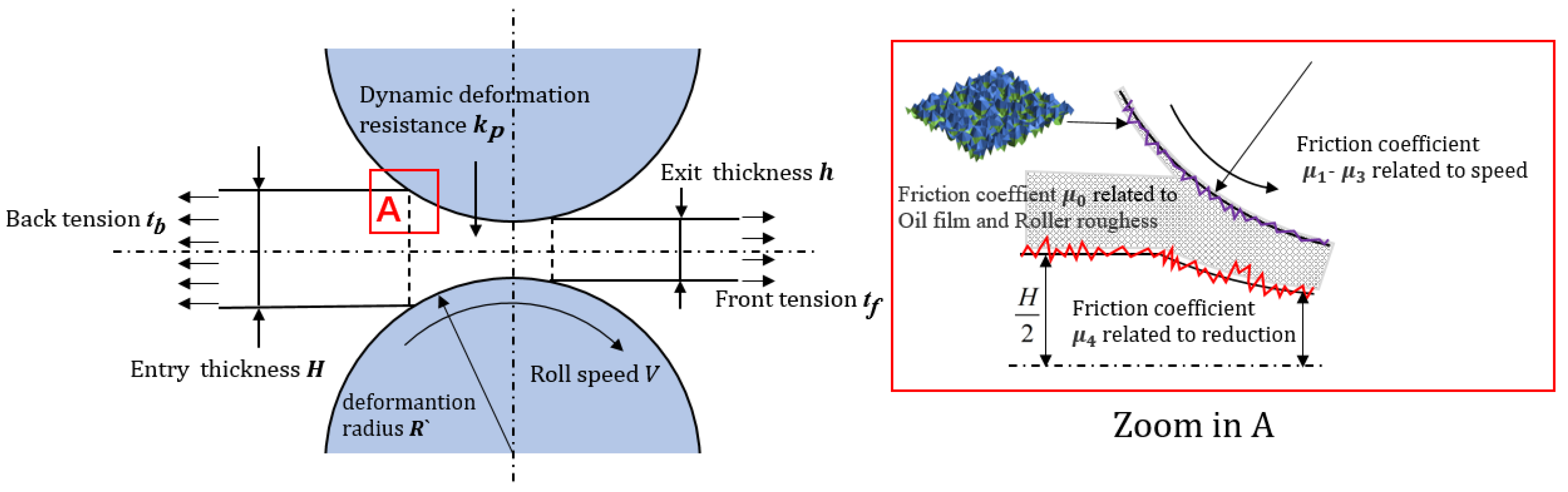
2. Theoretical Model of the Rolling Force

The research object of this paper is the 1720 mm 5-stand UCM TCM. Considering that the rolling force is not controlled by the rolling force model when the work roll of the S5 stand uses the dull roll, this paper only studies the RFPM of the S1 to S4 stands.

In the calculation of rolling force, the Bland–Ford model with a relatively rigorous theory is adopted. The calculation process of the model considers parameters such as the friction coefficient, elastic deformation of rolls, and strip tension, as shown in Figure 1. The equation is as follows:

$$\{\begin{array}{l}{P}_c=b\cdot K_p\cdot \kappa \cdot D_p\cdot \sqrt{R^{\prime }\cdot (H-h)}\cdot ZP\\ D_p=1.08+1.79\cdot r\cdot \sqrt{1-r}\cdot \mu \cdot \sqrt{\frac{R^{\prime }}{h}}-1.02\cdot r\\ \kappa =\left(1-\frac{t_b}{K_p}\right)\cdot \left(1.05+0.1\cdot \frac{1-\frac{t_f}{K_p}}{1-\frac{t_b}{K_p}}-0.15\cdot \frac{1-\frac{t_b}{K_p}}{1-\frac{t_f}{K_p}}\right)\\ ZP=\frac{P_a}{P_c}\end{array}$$

(1)

where P_c is the calculated rolling force, P_a is the measured rolling force, and κ is the influence coefficient of tension. Here, Dp is the influence coefficient of friction, T_f is the forward tension, T_b is the post-tension, b is the strip width, R′ is the radius of the work roll, K_p is the dynamic deformation resistance coefficient, ZP is the adaptive coefficient of the rolling force, and μ is the friction coefficient.

As shown in Equation (1), the dynamic deformation resistance coefficient, K_p, and the friction coefficient, μ, are very important for calculating the rolling force and seriously affect the calculation accuracy of the rolling force model.

2.1. Friction Coefficient Model

The friction coefficient model is shown in Equation (3). The friction coefficient, μ, is directly related to the lubrication characteristics of the emulsion. In addition, the change in rolling speed, roll surface roughness, strip length, reduction, and other factors will cause a change in the friction coefficient, μ. In this paper, the friction coefficient model parameters related to the change in lubrication conditions are considered, which is independent of the steel grade, so only μ₀ is optimized:

$$\mu =\left({\mu }_0+\frac{{\mu }_1}{v+{\mu }_2}+{\mu }_3\cdot v\right)\left(\frac{{\mu }_4}{1+N_r\cdot {\mu }_5}\right)$$

(2)

where μ₀ represents the lubrication conditions, μ₁, μ₂, μ₃, and μ₄ represent the rolling speeds, μ₅ is the rolling roll number, v is the rolling speed, and N_r is the number of rolling rolls after the roll change.

2.2. Deformation Resistance Model

In the calculation of deformation resistance, the influence of the initial mechanical properties of the strip, the deformation temperature, and the deformation rate during rolling should be considered. Therefore, the deformation resistance model is composed of static and dynamic terms, as shown in Equation (2).

In the ideal state, each steel grade should be associated with a set of static deformation resistance parameters. However, in production, the steel grade with an approximate YS is usually classified as a steel group, with the same static deformation resistance parameters. The dynamic deformation resistance coefficient, K_p, is linearly related to static deformation resistance, K_s, which is only associated with the mechanical properties of the material. When the new steel grade is produced or some of the original steel grade compositions are adjusted, there will be an unreasonable classification of steel groups. Therefore, this paper only considers optimizing the parameters in the K_s of all steel groups, as seen in Equation (3):

$$\{\begin{array}{l}{K}_p=K_s{(1000\cdot \stackrel{·}{\epsilon })}^{\alpha }\\ K_s=l\cdot {(\epsilon +m)}^n\\ \epsilon =\ln \{1/(1-r_t)\}\end{array}$$

(3)

where K_s is the static deformation resistance, α is the deformation rate sensitivity coefficient, $\stackrel{·}{\epsilon }$ is the strip deformation rate, l and m are the parameters of the static deformation resistance, n is the work-hardening coefficient, r_t is the average reduction rate, and ε is the true strain.

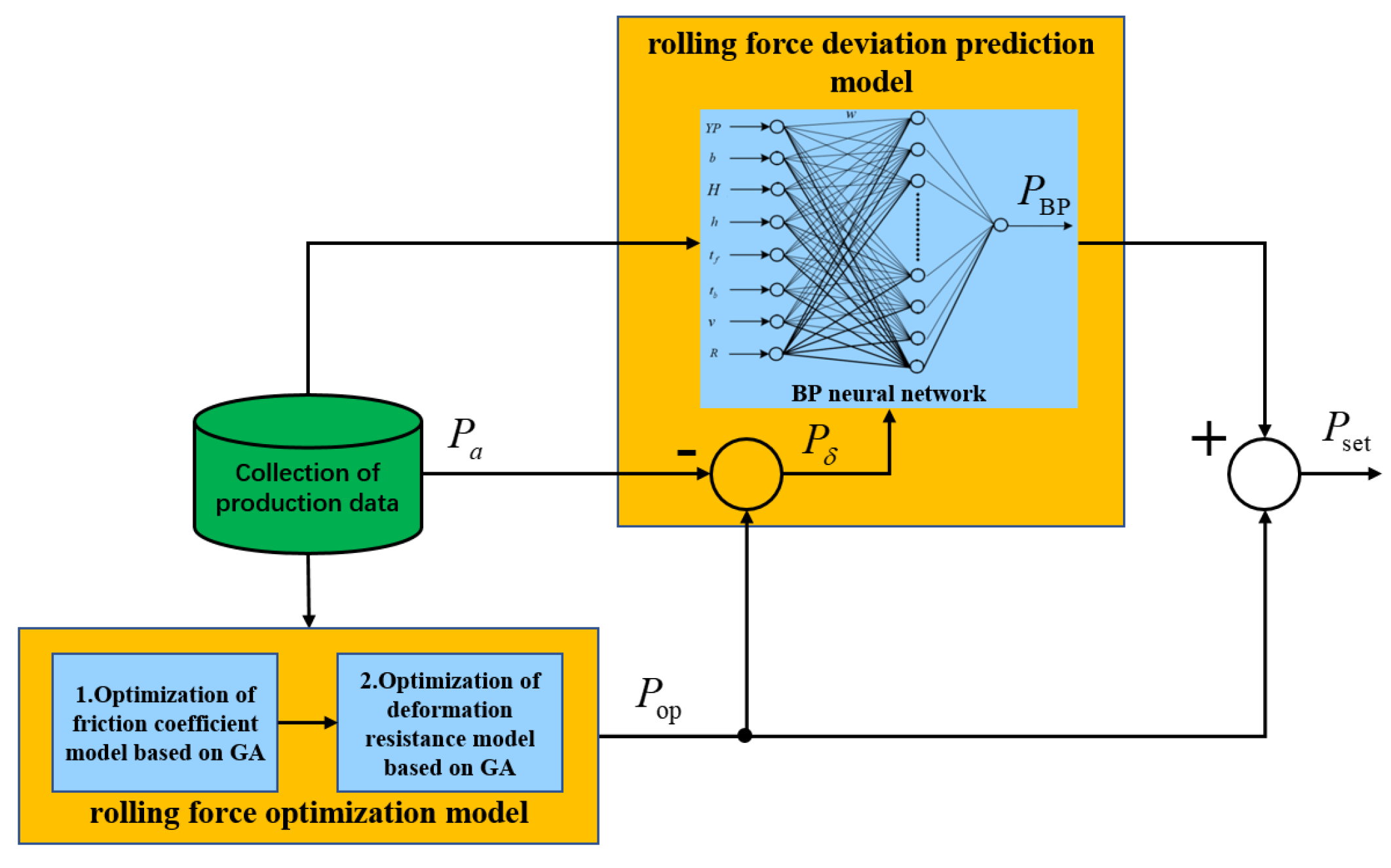
3. Rolling Force Preset Model (RPFM)

The RPFM consists of a rolling force optimization model (RFOM) and a rolling force deviation prediction model (RFDPM), as shown in Equation (4). The RFOM uses a GA to optimize the friction coefficient model and the deformation resistance model step by step. The RFDPM is established by a BP neural network, and the output of this model is the deviation between the measured values and the RFOM calculation result. The input is the measured process parameters. Figure 2 is the flow chart of the RPFM. The calculation uses the following equation:

$$\{\begin{array}{l}{P}_{set}=P_{BP}+P_{OP}\\ P_{\delta }=P_a-P_{OP}\end{array}$$

(4)

where P_set is the preset rolling force, P_BP is the rolling force deviation by the BP neural network, P_OP is the calculation rolling force after GA optimization, but not the best calculation result of each strip, and P_δ is the rolling force deviation.

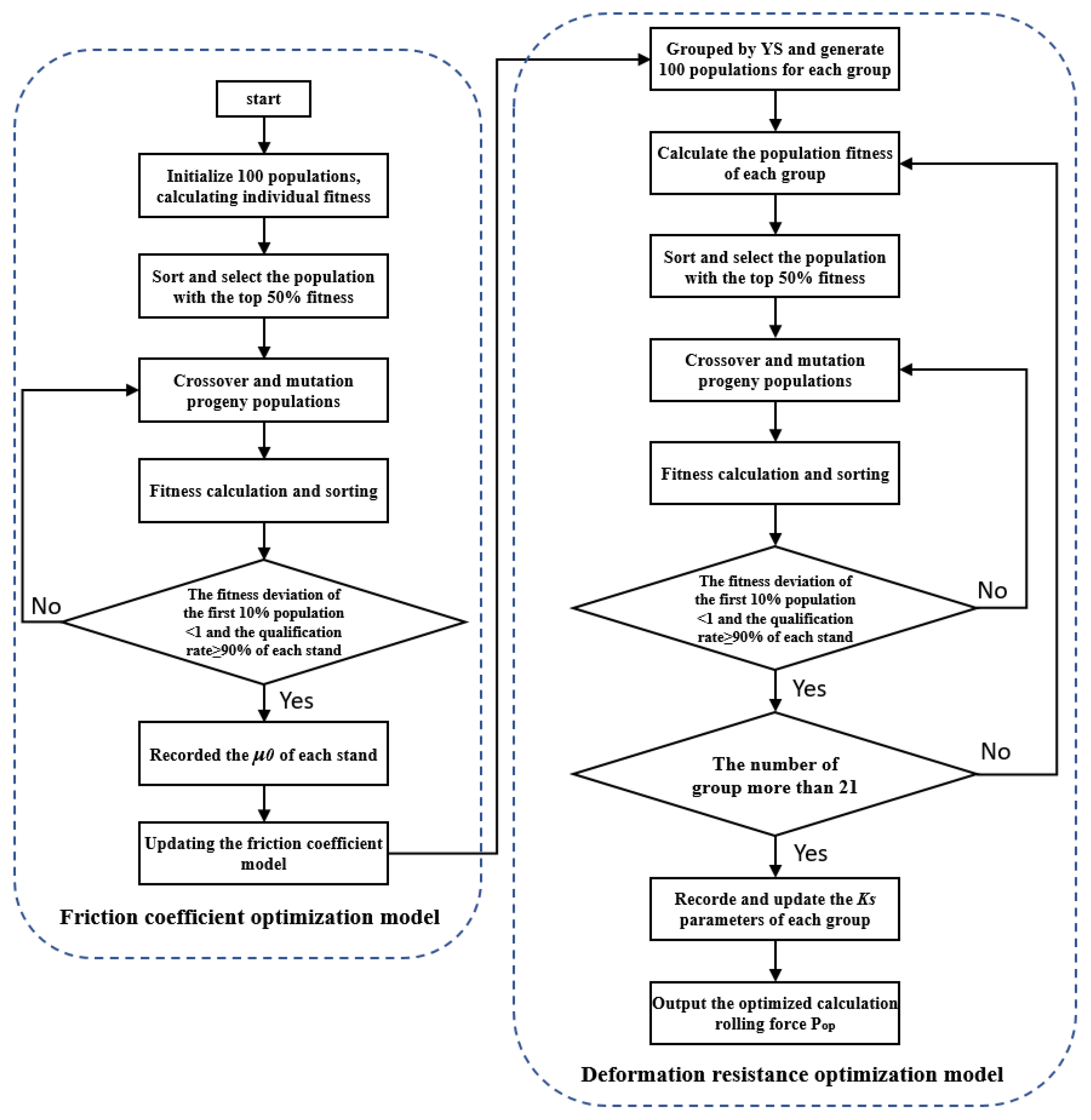
3.1. RFOM Established Based on GA

The RFOM adopts a real-coded GA to optimize the deformation resistance model and friction coefficient model. The calculation process includes population initialization, fitness calculation, fitness sorting, and new population generation by cross variation. The calculation process is shown in Figure 3.

The calculation process of each stand is the same except for the input parameters when calculating the rolling force, so the RFOM model will optimize the friction coefficient parameters of the four stands at the same time. The fitness function of the RFOM model is shown in Equation (5), and the approximation between the calculated value and the measured value is positively correlated with the F value. The RFOM model uses the measured production process data as input, in which the initial μ₀ of each stand and the initial l, m parameters of each steel group are collected from the cold-rolling L2 control system.

The variables of the initial population in the friction coefficient optimization model are μ₀ of the S1 to S4 stands. After 100 populations were initialized and the fitness was calculated, the top 50 populations with the best fitness were defined as the initial paternal population. With the method of crossing, 50 progeny populations were generated by the initial paternal population. The now 100 populations were sequenced according to fitness and generated new paternal populations, then the GA was repeated until the target converged. The optimization of the deformation resistance model was based on the new friction coefficient, and the deformation resistance model of each group was optimized by grouping the data according to the yield strength, using the following equation:

$$F={\displaystyle \sum _{j=1}^4{\displaystyle \sum _{i=1}^n|1-\frac{P_i^{j}a}{P_i^{j}c}|}}={\displaystyle \sum _{j=1}^4{\displaystyle \sum _{i=1}^n|1-Z{P}_i^j|}}$$

(5)

where n is the number for the calculation data.

3.2. An RFDPM Established Based on a BP Neural Network

3.2.1. BP Neural Network Theory

The BP neural network is a multilayer forward network based on the backpropagation algorithm, which has one input layer, one output layer, and several hidden layers. According to the approximation theory, a BP neural network with a nonlinear transfer function can realize nonlinear mapping with arbitrary precision when the number of hidden layer neurons is sufficient. For nonlinear processes and functions that only know input data and output data, the BP neural network can be used to train its input and output data with excellent fitting ability, so that the BP neural network can obtain a mapping function that is very close to the nonlinear process.

When the signal is transmitted forward, the output of each neuron is determined by the input of the neuron in the previous layer, so the signal calculation formula of the corresponding hidden-layer neuron and output-layer neuron are shown as follows, in Equations (6) and (7).

Hidden-layer neuron output:

$$H_i=f({\displaystyle \sum _{j=1}^m{w}_{ij}{x}_j}+b_i)$$

(6)

Output-layer neuron output:

$$Y_k=g({\displaystyle \sum _{i=1}^n{w}_{ki}{\mathrm{H}}_i}+s_k)$$

(7)

where f and g are the activation functions of the hidden layer and output layer; m and n are the input vector dimensions for the input layer and output layer; w_ij and w_ki are the weights of the input layer to the hidden layer and the weights of the hidden layer to the output layer, respectively; and b_i and s_k are the biases of the hidden layer and output layer, respectively.

Error backpropagation of the BP neural network is conducted using the gradient descent method. The loss function adopts the mean squared error (MSE) function, as shown in Equation (8). When the loss function reaches the target range or the expected value, the neural network’s learning ends:

$$Ep=\frac{1}{2P}\sum _{a=1}^P{({\displaystyle \sum _{k=1}^L{Y}_t^a-Y_k^a})}^2$$

(8)

where $Y_t^a$ and $Y_k^a$ are the target value and predicted value, respectively.

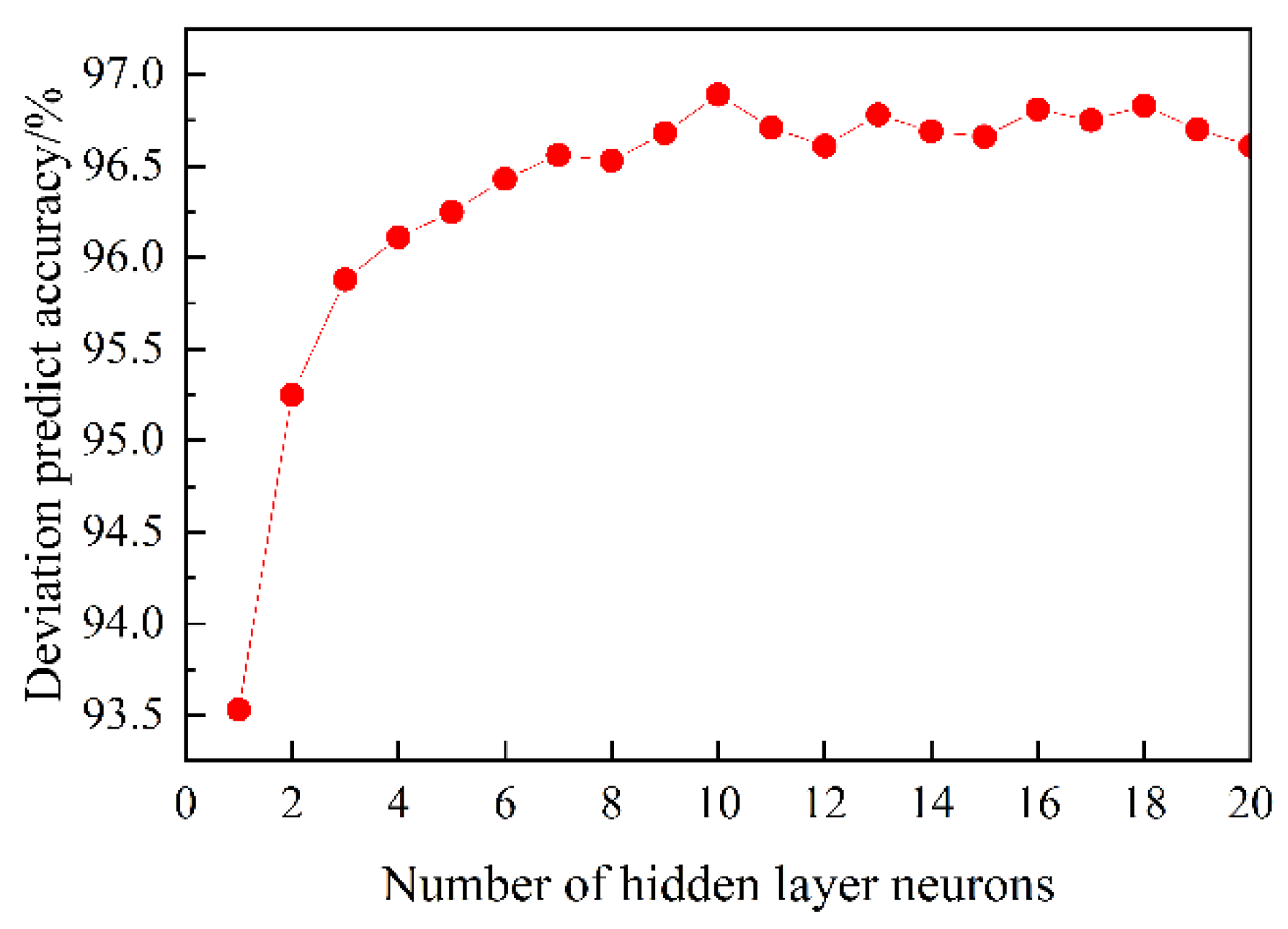
3.2.2. BP Neural Network Structure and Parameter Setting

The BP neural network is a typical supervised learning algorithm, so the parameters affecting the rolling force can be clearly established by analyzing the rolling force model. As shown in

Table 1. BP neural network input parameters.

No	Parameter	Unit	Min	Max
1	Yield strength	MPa	175	499
2	Strip width	mm	870	1595
3	Entry thickness of S1	mm	2.001	5.616
4	Exit thickness of S1	mm	1.316	4.65
5	Exit thickness of S2	mm	0.772	3.866
6	Exit thickness of S3	mm	0.508	3.011
7	Exit thickness of S4	mm	0.383	2.462
8	Exit speed of S1	mpm	53.7	426.70
9	Exit speed of S2	mpm	70.4	639.70
10	Exit speed of S3	mpm	104.6	969.4
11	Exit speed of S4	mpm	146.7	1203.70
12	Unit back tension of S1	MPa	2.04	7.93
13	Unit forward tension of S1	MPa	5.43	16.34
14	Unit forward tension of S2	MPa	6.19	19.11
15	Unit forward tension of S3	MPa	7.76	20.04
16	Unit forward tension of S4	MPa	8.76	22.58
17	Working roll radius of S1	mm	206.96	216.97
18	Working roll radius of S2	mm	195.04	216.78
19	Working roll radius of S3	mm	193.91	216.83
20	Working roll radius of S4	mm	192.95	207.09

, the 20-dimensional process parameters were selected from the cold rolling data to be the neural network input layer, with P_δ as the output layer, and the training result is P_BP. The training process of all stands is the same, and 8 parameters corresponding to the stand number are selected from the 20-dimensional parameters as the input layer for each stand training, so the number of input layers is 8.

Adopting the momentum optimization method for training, and using the ReLU as the activation function, the learning rate adopts 0.1 and the momentum term is 0.9. Due to the enormous differences in the orders of magnitude of the input parameters, to avoid adverse effects on the learning results, the min-max standardization method is adopted to normalize the data, as shown in Equation (9):

$$x_i=\frac{x-x_{min}}{x_{max}-x_{min}}$$

(9)

where x_max and x_min are the maximum and minimum numbers of the data sequences, respectively, and x_i is the normalization value of the data, i.

The computation accuracy and complexity of the BP neural network should be considered when selecting the number of hidden layer neurons. The number of neurons should be reduced as much as possible under the conditions of meeting the prediction accuracy of the model; otherwise, it will lead to overfitting of the BP neural network and reduce the generalization ability. As shown in Figure 4, when the number of neurons is 10, the model’s prediction accuracy begins to oscillate noticeably and no longer improves continuously, so the BP neural network has a topological structure of 8-10-1.

4. Analysis of the Calculation Results

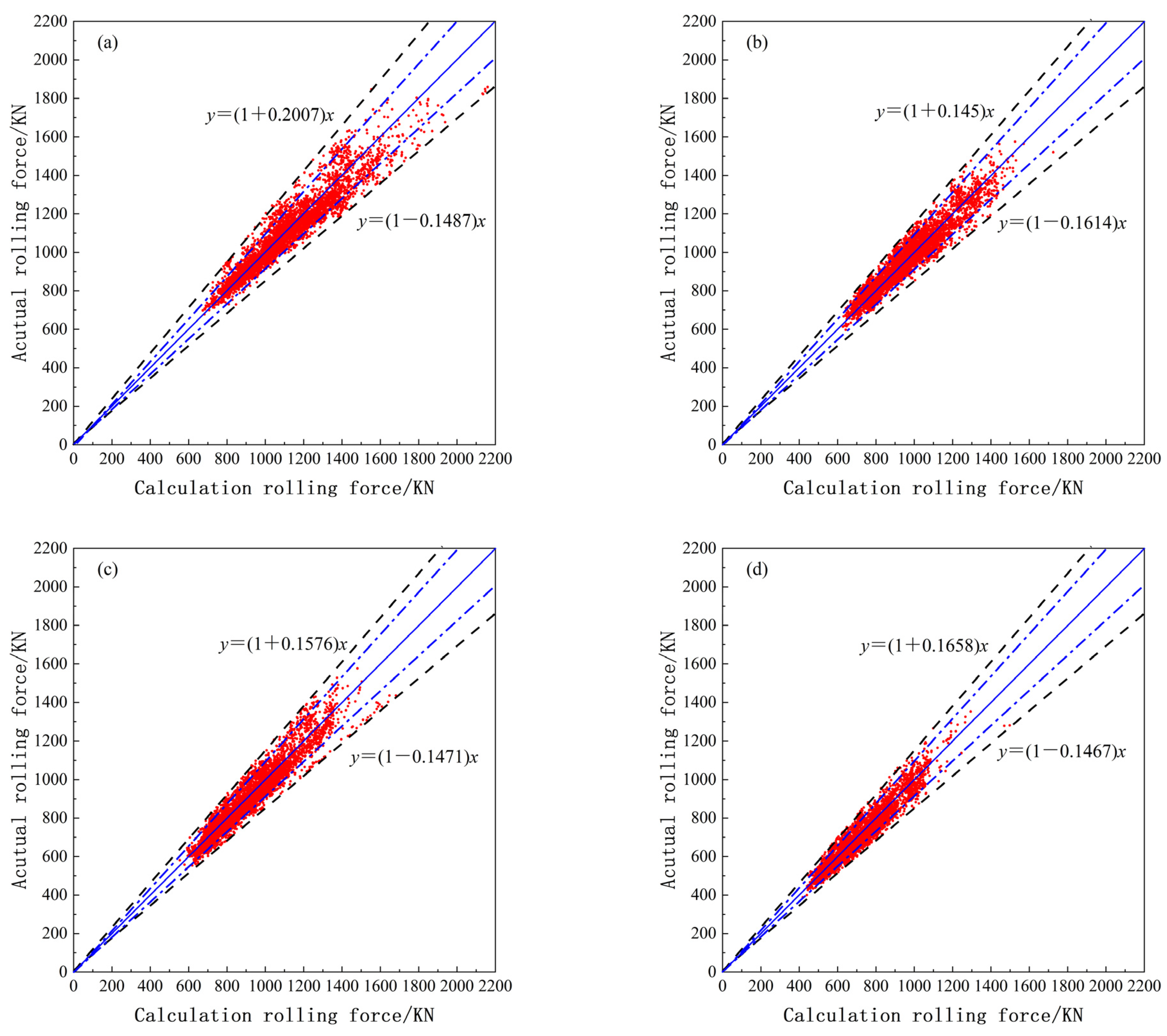
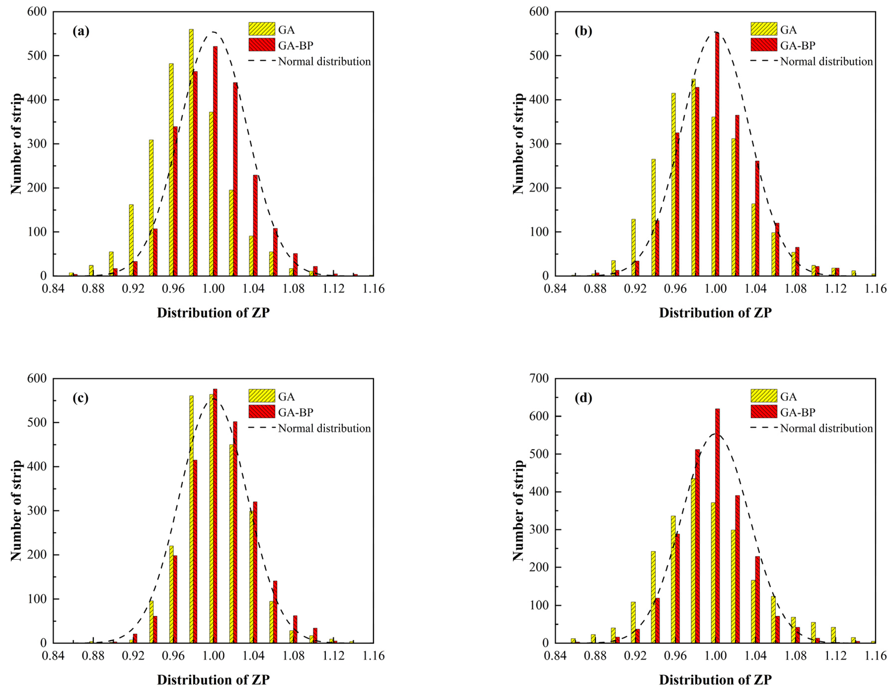
4.1. Calculation Result of RFOM

The calculated data were collected from the L2 control system, which could be divided into 21 groups according to YS, and 5000 data points, including all groups, were chosen to optimize the rolling force model after eliminating the abnormal data.

When |ZP − 1| ≤ 0.1, it is considered that the calculated value of rolling force is accurate and defines |ZP − 1|as the δ_ZP named rolling force adaptive deviation. The rolling force qualification rate, Φ_acc, is shown in Equation (10):

$$\{\begin{array}{l}{C}_{{}_i}^{(0.1)}=\{\begin{array}{l}1, \left|Z{P}_i-1\right|\le 0.1\\ 0, \left|Z{P}_i-1\right|>0.1\end{array}\\ {\varphi }_{acc}^{(0.1)}=\frac{{\displaystyle \sum _i^N{C}_{{}_i}^{(0.1)}}}{N}\end{array}$$

(10)

where $C_{{}_i}^{(0.1)}$ represents the statistics within the adaptive deviation’s acceptable range and the upper corner is the limit of deviation, and N is the number representing calculated data.

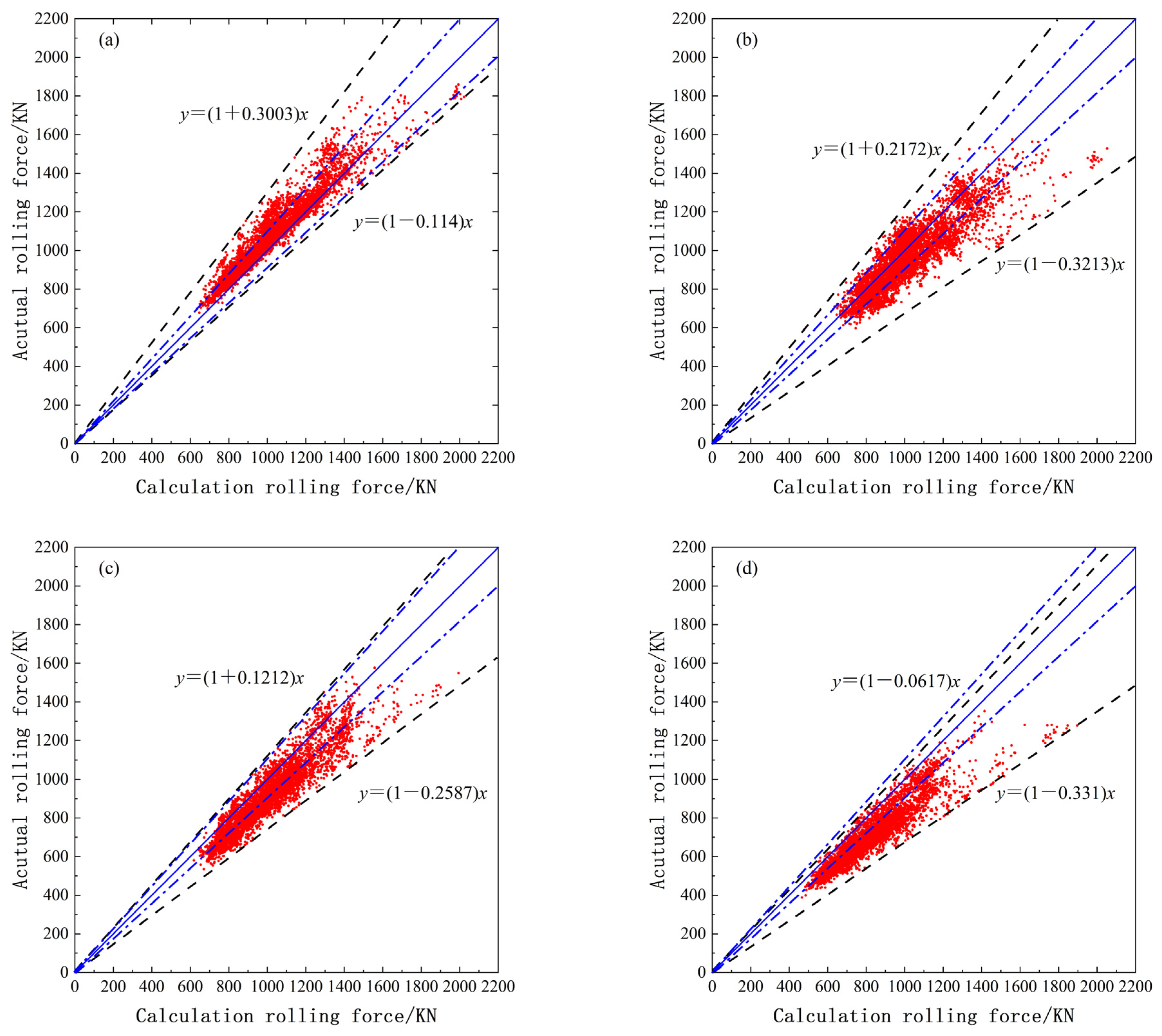
4.1.1. Rolling Force Model before Optimization

Figure 5 shows the calculated rolling force results of all stands before optimization, where the area surrounded by blue dotted lines is δ_ZP ≤ 0.1, and the solid blue line represents ZP = 1. It can be seen that the distribution of data points of each stand exceeds the range of blue dotted lines. The maximum ZP value of the S1 stand is 1.3003, and the minimum ZP of the S4 stand is 0.669.

As shown in Figure 6, the rolling force qualification rate ${\varphi }_{acc}^{(0.1)}$ of the S3 and S4 stands is less than 50%, among which the S4 stand is only 22.4%. Even compared with the range of δ_ZP ≤ 0.15, the qualification rate ${\varphi }_{acc}^{(0.15)}$ of the S4 stand is also less than 60%. The results show that the rolling force model currently used online can no longer meet the requirements of the high-precision rolling force preset.

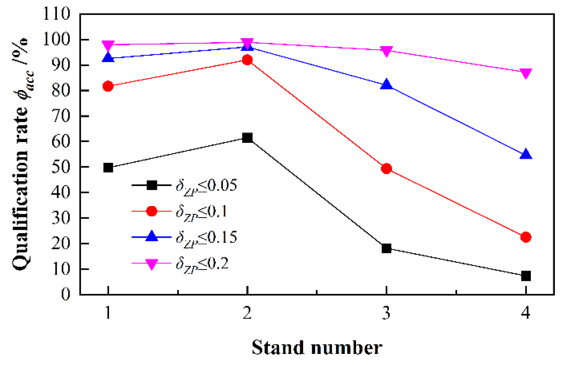
4.1.2. After Optimization of the Friction Coefficient Model

As shown in Figure 7, the distribution of the calculated rolling force has three obvious characteristics after optimizing μ₀:

(1) The maximum and minimum values of ZP have changed. Taking S2 as an example, the maximum and minimum ZP values before optimization are 1.2172 and 0.6787, respectively, but they become 1.1576 and 0.8529 after optimization. The optimization of μ₀ can effectively reduce the rolling force deviation.

(2) The ZP distribution is more compact. Obviously, the data distribution is significantly thinner than before optimization, and the dispersion of data decreases significantly.

(3) The data are concentrated around ZP = 1. The optimized rolling-force data are distributed on both sides of the solid line of ZP = 1, indicating that the optimized rolling force is closer to the expected value.

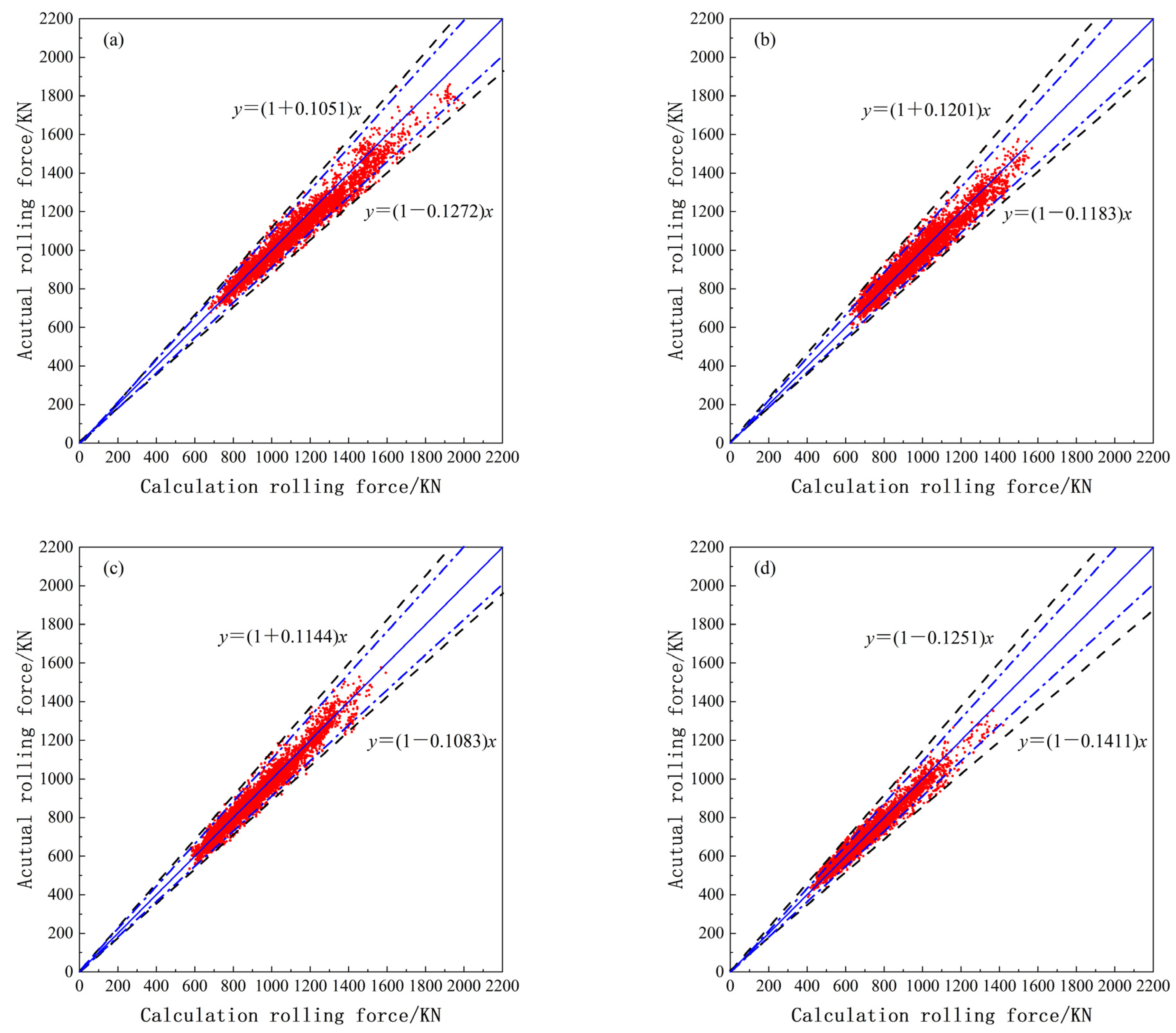
4.1.3. After Optimization of the Deformation Resistance Model

Either the steel component was adjusted or a new steel grade was developed to meet process improvement or market demand requirements. At this point, the original deformation resistance model coefficient is unsuitable, as it will lead to rolling-force deviation. Figure 8 shows that after the deformation resistance model is optimized, the degree of dispersion of the rolling force data is further reduced.

As shown in Figure 9, the qualification rate of δ_ZP ≤ 0.1 was improved significantly when the deformation resistance model was optimized. The S3 stand increased from 90.26% to 97.57%, and the S4 stand increased from 89.89% to 95.18%. Since δ_ZP ≤ 0.05 is a more stringent evaluation indicator, the qualification rate of the 4-stand average increased by 12.9% according to this indicator.

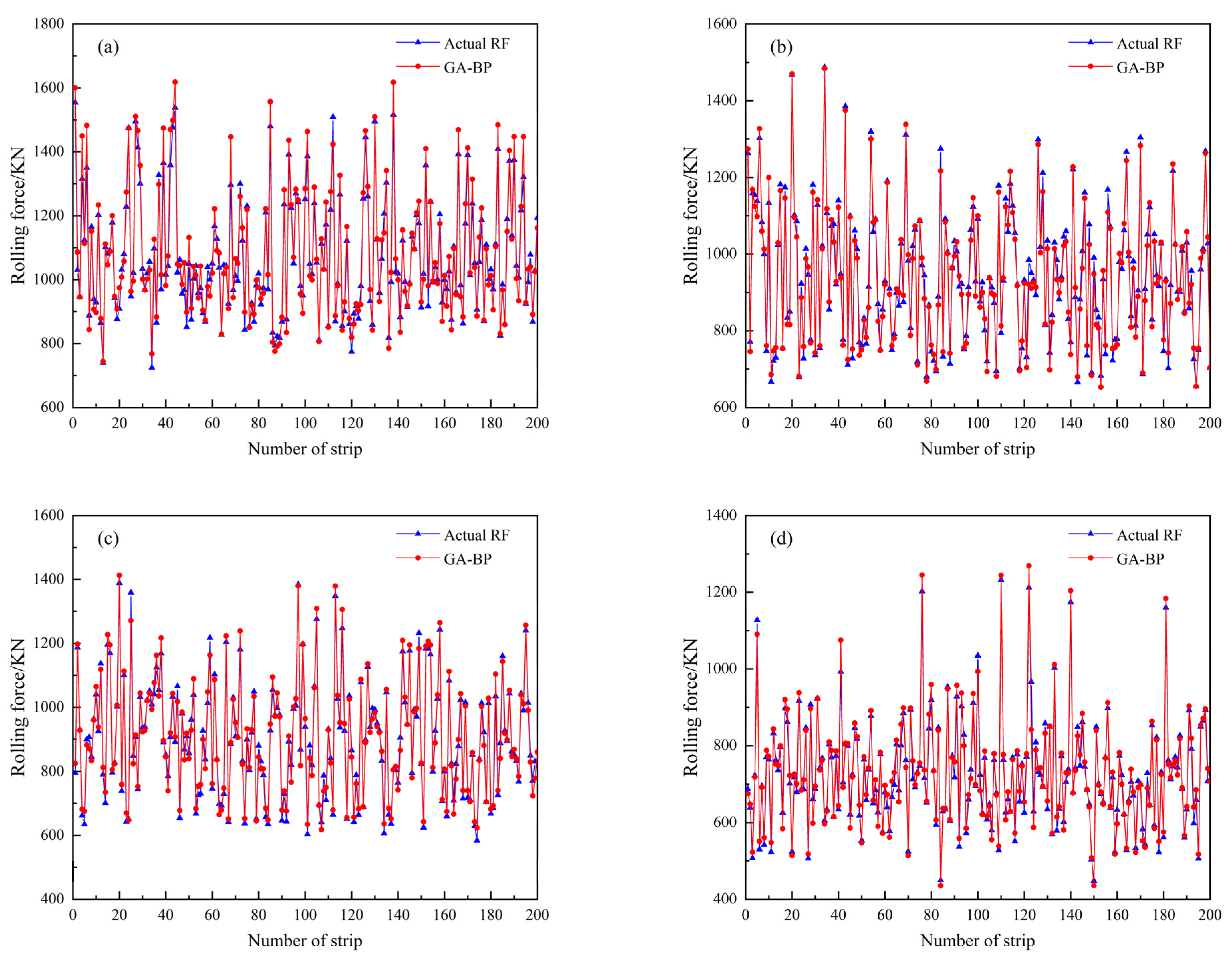
4.2. Calculation Result of RFDPM

BP neural network training also adopts 5000 data points; the ratio of the training set, test set, and verification set is 7:2:1. A standard normal distribution, with a mean value of 0 and a standard deviation of 1, was used for weight initialization and the number of training sessions was set to 50,000.

Two hundred groups of data were randomly selected from the calculated results compensated for by RFDPM and were compared with the actual values. As shown in Figure 10, although the actual rolling force of each stand varies widely, the deviation between the preset rolling force and the actual value remains small. As shown in

Table 2. Comparison of rolling force qualification rate, ${\varphi }_{acc}^{(0.1)}$.

	S1	S2	S3	S4	Average
Original(%)	81.64	91.98	49.37	22.49	61.37
GA(%)	96.45	95.87	97.57	95.18	96.27
GA-BP(%)	98.63	98.44	98.86	99.10	98.76

, the rolling force qualification rate ${\varphi }_{acc}^{(0.1)}$ was compared. Here, ${\varphi }_{acc}^{(0.1)}$ was further promoted after BP neural network compensation, and the average ${\varphi }_{acc}^{(0.1)}$ of the four stands increased from 96.27% to 98.76%.

Guo et al. [22] proved that the rolling force deviation presented a normal distribution. Therefore, to obtain a more accurate preset rolling force, the distribution of the rolling force adaptive deviation, δ_ZP ≤ 0.1, should conform to the three-sigma determinant criterion. Equation (11) calculates the probability density function of ZP. The histogram of the ZP value distribution from all stands after compensating for the rolling force with the BP neural network is shown in Figure 11, where the dotted line represents the normal distribution curve.

(1) The adaptive deviation δ_ZP of the rolling force after GA optimization is almost less than 0.1, but it is clear that in stands S1 and S2, part of the adaptive deviation is in the range of 0.92 to 0.96, which means that the accuracy of these calculated values is low. Similarly, data in the 0.98 to 1.02 range are less common in the S4 stand.

(2) The data compensated for by the BP neural network have a high degree of coincidence with the normal distribution. As shown in the

Table 3. Comparison of the rolling force qualification rate, ${\varphi }_{acc}^{(0.05)}$.

	S1	S2	S3	S4	Average
GA(%)	72.76	72.56	78.22	70.87	73.60
GA-BP(%)	86.49	79.60	87.07	91.09	86.06

, the average qualification rate, ${\varphi }_{acc}^{(0.05)}$, of the GA method is 73.60%, while the GA-BP method increases to 86.06% after statistical analysis where δ_ZP ≤ 0.05. Thus, the preset rolling force compensated for by the BP neural network has higher accuracy.

$$f(ZP)=\frac{1}{\sqrt{2\pi (\frac{1}{30})}}\exp (-\frac{{(ZP-1)}^2}{{(\frac{1}{30})}^2})$$

(11)

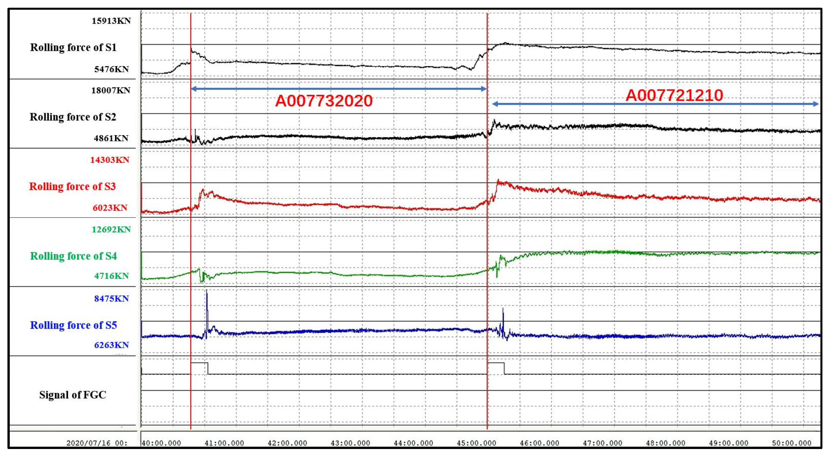
5. Industrial Applications of RFPM

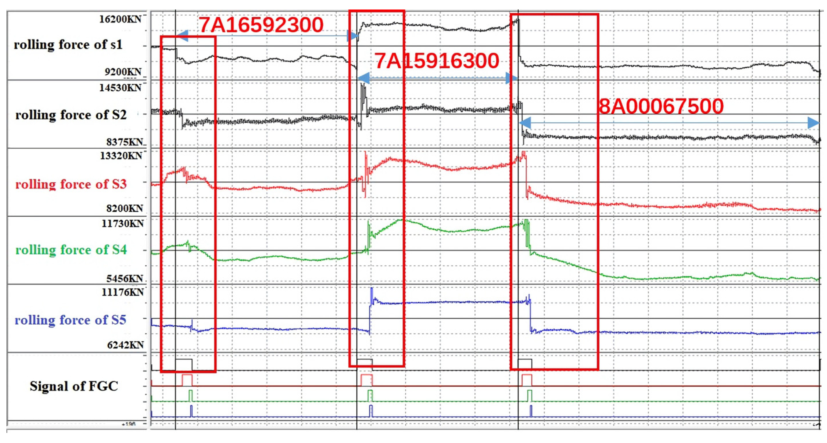
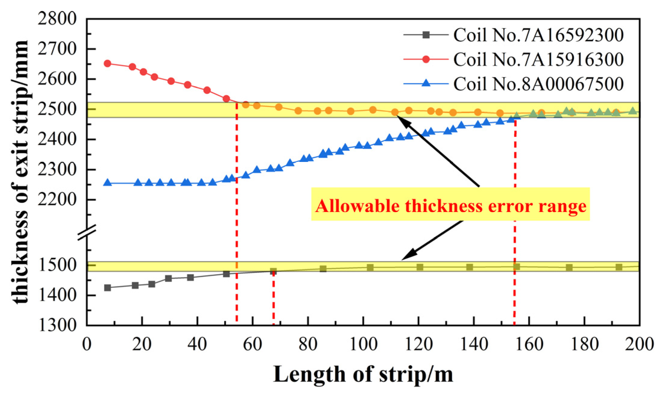
5.1. Thickness Defect Analysis of the Strip Head before Optimization

If the actual thickness of the strip deviates from the target thickness by more than 1%, the strip is considered to have a thickness defect. Some of the FGC strips before optimization are shown in

Table 4. The FGC strip before optimization.

Coil	Steel Grade	Strip Width/mm	Entry Thickness/mm	Exit Thickness/mm	YS/MPa	Length of Thickness Defect/m
7A16592300	SPHD	1340	4541	1495	225	67.5
7A15916300	LG280VK	1295	4873	2500	391	53.5
8A00067500	SPHC-B	1300	5347	2500	225	153.5

, and Figure 12 shows the strip head thickness defect. It was evident that a large thickness defect was prevalent in the strip heads after FGC was executed.

The actual rolling-force curve of strip steel is shown in Figure 13. The rolling force of the S3 and S4 stands after FGC is different from that in the high-speed rolling stage, so it takes a long time to adjust. According to the roll-gap model shown in Equation (12), if AGC executes the closed-loop adjustment of rolling force for a long time period, the roll gap adjustment speed will also be affected, which will result in the actual thickness of the strip not being controlled quickly enough to achieve the target value. Hence:

$$g=h_{i+1}-\left(\frac{p}{K_s}+\xi -{\delta }_0\right)+g_z+g_{zm}-c_1+s_l$$

(12)

where ζ is the roll surface stiffness coefficient, p is the rolling force, h_i+1 is the exit strip thickness, M_s is the mill’s longitudinal stiffness, δ₀ is the oil film thickness, g_z is the zeroing gap, g_m is the zeroing gap spring value, c₁ is the constant, and s_l is the self-learning value of the gap.

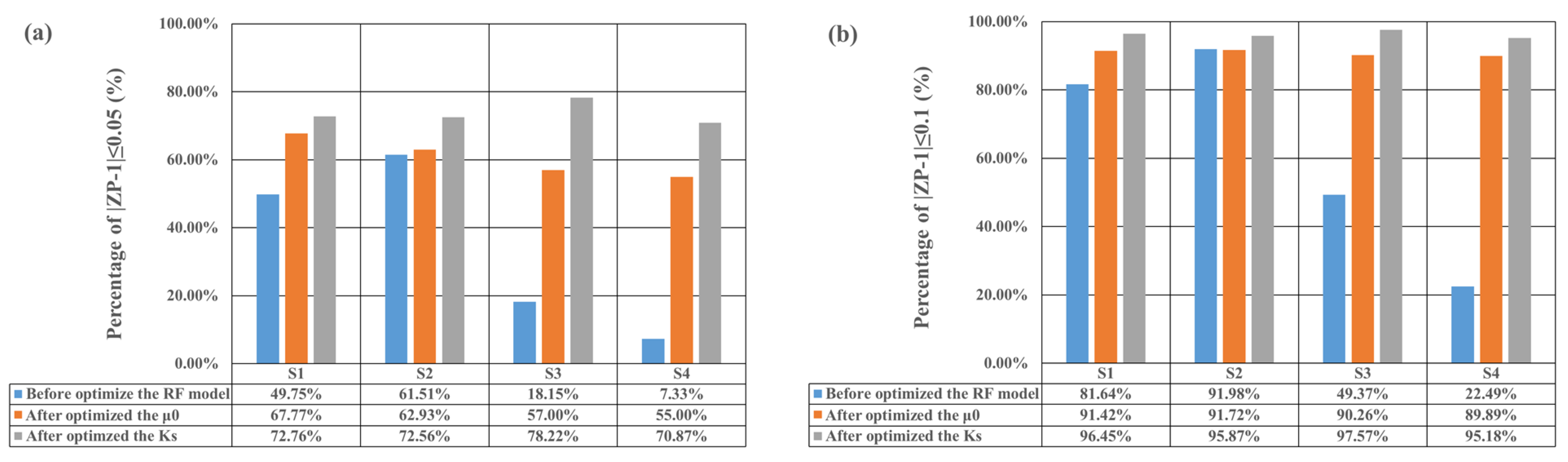
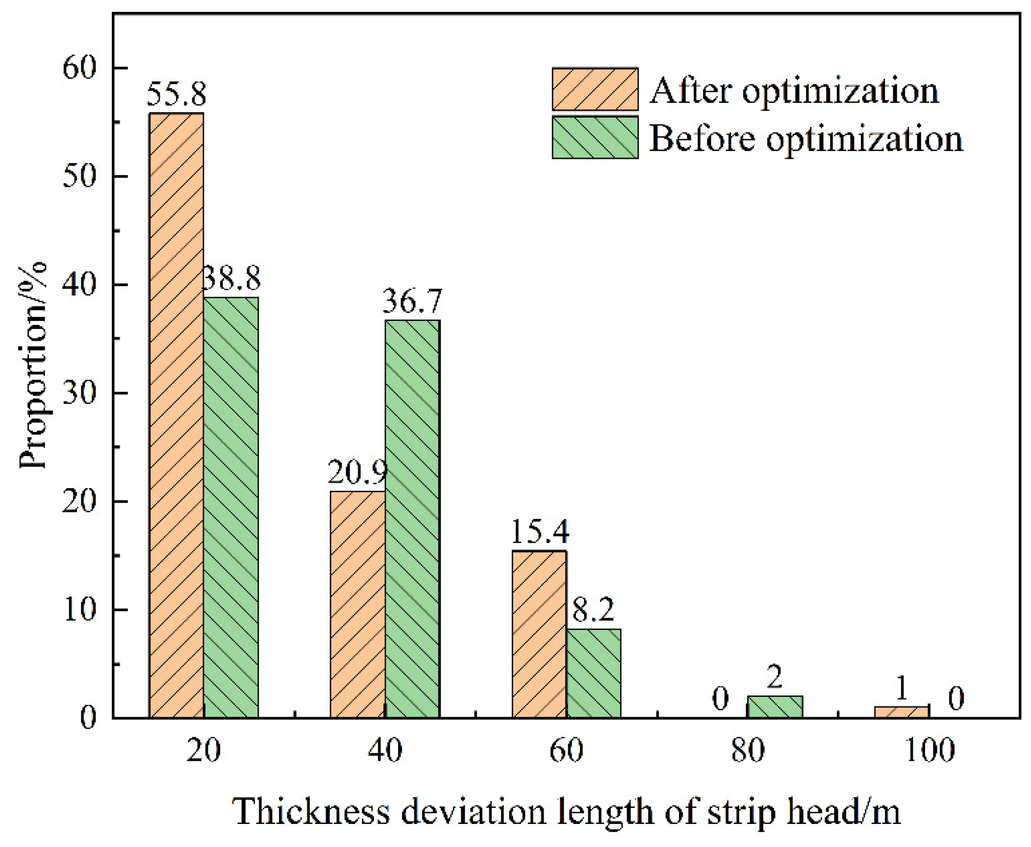
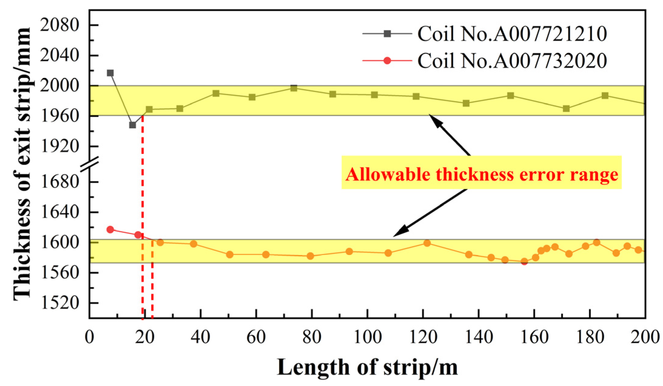
5.2. Optimization Effect Analysis

As shown in Figure 14, the deviation between the rolling force set on stands 3 and 4 and the rolling force at the high-speed rolling stage is small, so the closed-loop adjustment of the rolling force after FGC is more rapid, which can stabilize the rolling force in a short time and effectively reduce the head-thickness defect. As shown in Figure 15 and

Table 5. The FGC strip after optimization.

Coil	Steel Grade	Strip Width/mm	Entry Thickness/mm	Exit Thickness/mm	YS/MPa	Length of Thickness Defect/m
A007732020	40Mn-C	1230	2076	1590	467	19.5
A007721210	S50-A	1210	2468	2004	435	23.5

, the lengths of the strip head-thickness defect exceeding the allowable range for coils A005338710 and A007732020 after FGC are only 21.5 and 23.5 m, respectively.

After optimizing the preset rolling force, the average thickness defect length of the strip head is shortened from 47.3 m to 29.6 m. As shown in Figure 16, the proportion of defective lengths of less than 20 m increases from 38.8% to 55.8%, and the proportion between 20–40 m decreases from 36.7% to 20.9%. The defects of thickness over 60 m are also greatly improved. Therefore, the thickness defect length of the strip head can be effectively reduced by optimizing the rolling force model; this method is useful for all steel grades.

6. Conclusions

(1). The GA method is used to optimize the friction coefficient model and the deformation resistance model in the rolling-force theoretical model. The optimization results show that the average ${\varphi }_{acc}^{(0.1)}$ of the four stands increased from 61.37% to 96.27%, and the ${\varphi }_{acc}^{(0.1)}$ of the S4 stand increased from 22.49% to 95.18%. The calculation accuracy of the rolling force theoretical model is, therefore, significantly improved.

(2). After compensating for the RFOM with a BP neural network, the RFPM was established. The GA-BP method improves the average ${\varphi }_{acc}^{(0.1)}$ of four stands, from 96.27% to 98.76%, and makes the rolling-force deviation distribution consistent with the normal distribution, in which ZP follows N(1,(1/30)²). In this case, the preset rolling force has high accuracy and high precision.

(3). After applying the RFPM, the deviation between the preset rolling force and the actual rolling force is effectively reduced, so that the closed-loop adjustment time of the rolling force is also reduced. After FGC, the proportion of thickness defect lengths of less than 20 m increases from 38.8% to 55.8%, and the proportion between 20–40 m decreases from 36.7% to 20.9%.

References

1. Ren, L.; Zhou, S.; Peng, T.; Ou, X. A review of CO2 emissions reduction technologies and low-carbon development in the iron and steel industry focusing on China. Renew. Sustain. Energy Rev. 2021, 143, 110846. [Google Scholar] [CrossRef]
2. Chubenko, V.; Khinotskaya, A.; Yarosh, T.; Saithareiev, L. Sustainable development of the steel plate hot rolling technology due to energy-power process parameters justification. E3S Web Conf. 2020, 166, 06009. [Google Scholar] [CrossRef]
3. Yamashita, M.; Yarita, I.; Abe, H.; Mikuriya, T.; Yanagishima, F. Technologies of flying gauge change in fully continuous cold rolling mill for thin gauge steel strips. In Proceedings of the 4th International Steel Rolling Conference—The Science and Technology of Flat Rolling, Deauville, France, 1–3 June 1987; Volume 2. [Google Scholar]
4. Kijima, H.; Kenmochi, K.; Yarita, I.; Sunamori, Y.; Fukuhara, A.; Miyahara, M. Improvement of the accuracy in thickness during flying gauge change in tandem cold mills. Rev. Métall. 1998, 95, 911–918. [Google Scholar] [CrossRef]
5. Wang, J.; Jiang, Z.; Tieu, A.; Liu, X.; Wang, G. A flying gauge change model in tandem cold strip mill. J. Mater. Process. Technol. 2008, 204, 152–161. [Google Scholar] [CrossRef]
6. Li, S.; Wang, Z.; Guo, Y. A novel analytical model for prediction of rolling force in hot strip rolling based on tangent velocity field and MY criterion. J. Manuf. Process. 2019, 47, 202–210. [Google Scholar] [CrossRef]
7. You, G.; Li, S.; Wang, Z.; Yuan, R.; Wang, M. A novel analytical model based on arc tangent velocity field for prediction of rolling force in strip rolling. Meccanica 2020, 55, 1453–1462. [Google Scholar] [CrossRef]
8. Peng, W.; Ding, J.G.; Zhang, D.H.; Zhao, D.W. A novel approach for the rolling force calculation of cold rolled sheet. J. Braz. Soc. Mech. Sci. Eng. 2017, 39, 5057–5067. [Google Scholar] [CrossRef]
9. Liu, S.; Lu, H.; Zhao, D.; Huang, R.; Jiang, J. Dynamic rolling force modeling of cold rolling strip based on mixed lubrication friction. Int. J. Adv. Manuf. Technol. 2020, 108, 369–380. [Google Scholar] [CrossRef]
10. Rath, S.; Singh, A.P.; Bhaskar, U.; Krishna, B.; Santra, B.K.; Rai, D.; Neogi, N. Artificial Neural Network Modeling for Prediction of Roll Force During Plate Rolling Process. Mater. Manuf. Process. 2010, 25, 149–153. [Google Scholar] [CrossRef]
11. Teng, W.; Wang, G.M. Rolling Force Prediction System of Cold Rolling Process Based on BP Neural Network. Adv. Mater. Res. 2013, 690–693, 2361–2365. [Google Scholar] [CrossRef]
12. Bagheripoor, M.; Bisadi, H. Application of artificial neural networks for the prediction of roll force and roll torque in hot strip rolling process. Appl. Math. Model. 2013, 37, 4593–4607. [Google Scholar] [CrossRef]
13. Zhang, S.H.; Che, L.Z.; Liu, X.Y. Modelling of Deformation Resistance with Big Data and Its Application in the Prediction of Rolling Force of Thick Plate. Math. Probl. Eng. 2021, 2021, 2500636. [Google Scholar] [CrossRef]
14. Xin-Qiu, Z.; Yan-Sheng, W. BP neural network based GPSA used in tandem cold rolling force prediction. In Proceedings of the 2011 International Conference on Consumer Electronics, Communications and Networks (CECNet), Xianning, China, 16–18 April 2011; pp. 4829–4832. [Google Scholar] [CrossRef]
15. Wang, Z.-H.; Gong, D.-Y.; Li, X.; Li, G.-T.; Zhang, D.-H. Prediction of bending force in the hot strip rolling process using artificial neural network and genetic algorithm (ANN-GA). Int. J. Adv. Manuf. Technol. 2017, 93, 3325–3338. [Google Scholar] [CrossRef]
16. Zheng, G.; Ge, L.-H.; Shi, Y.-Q.; Li, Y.; Yang, Z. Dynamic Rolling Force Prediction of Reversible Cold Rolling Mill Based on BP Neural Network with Improved PSO. In Proceedings of the 2018 Chinese Automation Congress (CAC), Xi’an, China, 30 November–2 December 2018; pp. 2710–2714. [Google Scholar] [CrossRef]
17. Sun, S.; Zhang, J.; Wang, J.; Xu, L. The Application of New Adaptive PSO in AGC and AFC Combination Control System. Procedia Eng. 2011, 16, 702–707. [Google Scholar] [CrossRef] [Green Version]
18. Jansen, M.; Broese, E.; Feldkeller, B.; Poppe, T. How neural networks are proving themselves in rolling mill process control. Met. Min. More 1999, 1, 4–6. [Google Scholar]
19. Zhang, Q.D.; Xu, X.G.; Yu, M.; Zhai, B.; Li, S. Cold Rolling Force Model Based on GA and ANN for Stainless Steel Strip. Iron Steel 2018, 43, 46–48. [Google Scholar] [CrossRef]
20. Cui, C.G. Intelligent prediction model based on neural network algorithm and mechanism model for rolling force in tandem cold rolling. Comput. Mod. 2019, 8, 74–78, 91. [Google Scholar] [CrossRef]
21. Zhang, S.H.; Deng, L.; Che, L.Z. An integrated model of rolling force for extra-thick plate by combining theoretical model and neural network model. J. Manuf. Process. 2022, 75, 100–109. [Google Scholar] [CrossRef]
22. Guo, H.; Hao, P.; Chen, J. Based on Support Vector Machine of Cold Rolling Force Prediction Research. DEStech Trans. Comput. Sci. Eng. 2018, 197–204. [Google Scholar] [CrossRef]
Figure 1. The deformation zone of the roll gap.
Metals 12 00924 g001
Figure 2. The calculation process of the RPFM.
Metals 12 00924 g002
Figure 3. Calculation process of RFOM, based on the GA.
Metals 12 00924 g003
Figure 4. The effect of hidden-layer neuron numbers.
Metals 12 00924 g004
Figure 5. Rolling force calculation results distribution before optimization: (a) S1 stand, (b) S2 stand, (c) S3 stand, (d) S4 stand.
Metals 12 00924 g005
Figure 6. Rolling force qualification rate of each stand.
Metals 12 00924 g006
Figure 7. Rolling force calculation results distribution after optimizing the friction coefficient model: (a) S1 stand (b) S2 stand (c) S3 stand (d) S4 stand.
Metals 12 00924 g007
Figure 8. Rolling force calculation result distribution after the optimized deformation resistance model: (a) S1 stand, (b) S2 stand, (c) S3 stand, and (d) S4 stand.
Metals 12 00924 g008
Figure 9. Comparison of rolling force qualification rates: (a) δZP ≤ 0.05, and (b) δZP ≤ 0.1.
Metals 12 00924 g009
Figure 10. Comparison of the rolling force between the actual value and preset value: (a) S1 stand, (b) S2 stand, (c) S3 stand, (d) S4 stand.
Metals 12 00924 g010
Figure 11. The histogram of the ZP value distribution between GA and GA-BP: (a) S1 stand, (b) S2 stand, (c) S3 stand, (d) S4 stand.
Metals 12 00924 g011
Figure 12. Thickness defect of the strip head before optimization.
Metals 12 00924 g012
Figure 13. Rolling force of each stand before optimization.
Metals 12 00924 g013
Figure 14. The rolling force of each stand after optimization.
Metals 12 00924 g014
Figure 15. Thickness defect of the strip head after optimization.
Metals 12 00924 g015
Figure 16. The proportion of thickness defects after optimization.
Metals 12 00924 g016