Article

Bending Behaviour Analysis of Aluminium Profiles in Differential Velocity Sideways Extrusion Using a General Flow Field Model

1
Department of Mechanical Engineering, Imperial College London, London SW7 2AZ, UK
2
Department of Mathematics, Imperial College London, London SW7 2AZ, UK
*
Author to whom correspondence should be addressed.
Metals 2022, 12(5), 877; https://doi.org/10.3390/met12050877
Submission received: 2 May 2022 / Revised: 18 May 2022 / Accepted: 19 May 2022 / Published: 21 May 2022

Abstract

:
The work in this paper concerns an analytical model for quantitatively describing the bending behaviour of aluminium profiles produced in a novel extrusion process: the differential velocity sideways extrusion (DVSE), in which two opposing rams with a velocity of v 1 and v 2 were employed, respectively. The analytical model was built on the basis of the upper bound theorem utilising a general streamline equation controlled by a shape factor n, and the curvature was calculated using the material flow velocity gradient across the die exit orifice. The predicted material flow velocity across the die exit orifice, and extrudate curvature agreed well with the finite element (FE) modelling results, which were found to be irrespective of the shape factor n of the streamline equation. For a given extrusion ratio, the minimum value of n = 2 leads to the minimum and closest theoretical extrusion pressure, the n value for obtaining the best approximated mean effective strain of the extruded profile increases with the increase of the velocity ratio v 2 / v 1 , and the value of n = 3.5 gives the closest mean effective strain as a whole.

1. Introduction

Aluminium alloy has found its extensive applications as a structural element in the transport industry, due to its good combination of light weight and high strength. When utilising lightweight aluminium components on aircraft, trains and cars, a reduced consumption of energy and therefore a decreased emission of CO2 can be achieved, which is becoming increasingly important in mitigating the potential supply shortage of non-emitting electricity and achieving net-zero emissions by 2050 [1,2,3,4]. In industry, ultra-light structures with highly complicated morphology have been mostly manufactured by using curved aluminium alloy profiles with various cross-sections as constructional elements [5,6,7,8]. Since little machining and welding efforts are needed when using curved aluminium profiles to construct lightweight structures, greatly improved aerodynamic properties and time and space savings can be achieved [9,10,11,12].
Current forming methods for curved profiles are mostly achieved by bending straight extrusion profiles using conventional cold bending methods, such as roll bending, rotary draw bending, stretch bending and press bending [5,13]. Much research has been done on conventional cold bending methods, with an aim of minimising or avoiding defects such as springback of profiles and cross-sectional distortion during the bending process [5,14]. One effective approach is the superposition of external stress with conventional bending methods, such as compression superposed three-roll-bending and torque superposed spatial bending [15,16,17,18]. It was reported that the springback and cross-section distortion of curved profiles can be reduced due to the superposition of compressive stress or torsion with external bending moment [16,19,20,21,22].
Some extrusion-bending integrated techniques have been proposed to reduce the procedures of manufacturing curved profiles. The first one is curved profile extrusion (CPE) [23,24], during which a curved profile can be directly formed from a billet in one extrusion procedure, thus greatly improving the production efficiency. CPE is developed on the basis of the conventional forward extrusion method, and an external device is utilised near the die orifice to deflect/bend the profile being extruded. The curvature of the profile coming out of the die orifice is controlled by the external bending device. Muller et al. [25,26] used a segmented regulating guiding device which is composed of serially placed bending discs at the die exit, to achieve bending of the extruded profile. Since the curvature is generated at the die exit where the material is still in the fully plastic state, this forming process produces profiles/sections with no springback, reduced residual stresses, minimal cross-sectional distortion and nearly no decrease in the forming ability [27,28]. Another way of achieving extrusion-bending integration is by exploiting an inclined rotary die for producing curved bars and tubes [29,30,31], where a billet is extruded through a die aperture inclined towards the central axis of the container at a predetermined angle. It was found that by adjusting the inclination angle of the die aperture, the curvature of the extruded bars and tubes can be continuously varied, and the curvature increases with the increase of inclination angle.
The authors have proposed a new extrusion-bending integrated method, differential velocity sideways extrusion (DVSE) [32]. The basic principle of this method is that profiles are extruded and bent simultaneously in an extrusion die orifice due to a velocity gradient across the cross-section of the extrudate. The velocity gradient is achieved by controlling the velocities of rams at each end of the billet (see Figure 1a). It has been shown that by adjusting the extrusion velocity ratio of the two opposed rams, curved profiles with adjustable curvatures can be formed in one extrusion-bending procedure, and the intense deformation in DVSE results in a greatly refined microstructure and good mechanical properties of the formed profiles [33,34]. The upper bound method has been widely employed to analyse the deformation characteristics and predict the forming force/pressure in various metal forming processes, including forging, ring rolling and extrusion of non-symmetrical profiles with minimised curvature [35,36,37,38,39,40,41]. The simple shear model has been utilised in the upper bound theorem for simplicity where a number of velocity discontinuity surfaces are assumed; material flow velocity experiences abrupt variations when passing through the velocity discontinuity surfaces [42,43,44,45,46]. However, in practice the material does not suddenly change its velocity when passing through an infinitesimal surface. An analytical model for analysing the DVSE process has been proposed based on the simple shear model, in which the plastic deformation zone (PDZ) was divided into several single shear planes and the deformation mode was considered as rigid blocks of material separated by the velocity discontinuity planes [47]. Although velocity discontinuities are allowable in the upper bound method, the actual material flow in the PDZ is continuous without velocity discontinuity. For a better understanding of the forming characteristics of the DVSE process, an analytical model utilising a more general form of continuous flow line model is developed in this paper, which is able to be simplified to the simple shear model and provide a more accurate prediction of the extrudate bending behaviour.
In this work, the bending behaviour of the AA1050 aluminium alloy profiles in the DVSE process has been analysed using a general flow field model, in which any point of the material in the PDZ is described by a continuous velocity filed. The effects of the shape factor n of the flow field model on the distribution of the material flow velocity across the die orifice, extrudate curvature, extrusion pressure and mean effective strain of the extruded AA1050 profiles during the novel DVSE process were investigated in detail. Finite element (FE) modelling was also conducted to validate the analytical model and facilitate the understanding of fundamental properties of the DVSE process.

2. Materials and Methods

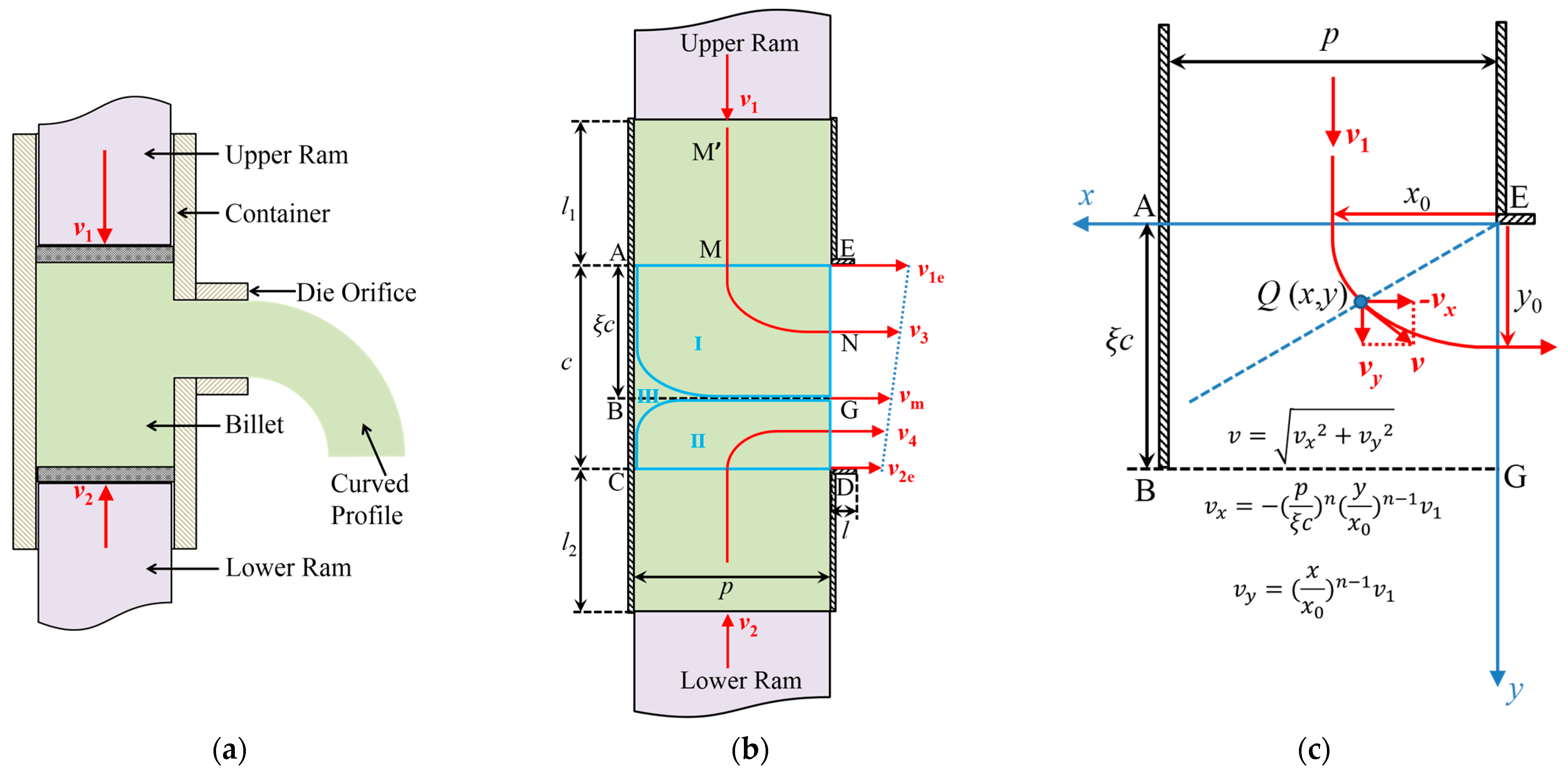
2.1. Theoretical Model

The schematic of the DVSE process is shown in Figure 1a, where a billet is extruded sideways through a die orifice by two opposing rams. The extrusion pressure and velocity of the ram are P 1 ,   v 1 and P 2 ,   v 2 , respectively. In this work, a plane strain configuration is considered where the container and die orifice have the same thickness (normal to the paper), and strain along the thickness direction is assumed to be zero [48]. Figure 1b illustrates the deformation model diagram, where the width of the billet (entrance channel) and the extruded profile (exit channel) is p and c , respectively. The material in the channel intersection region is divided into three regions. Regions I and II are the plastic deformation zone (PDZ) and region III is the dead metal zone (DMZ). Line BG passing through the vertex of the DMZ can be drawn, which divides the PDZ and extrudate into two parts coming from the two rams, respectively [32,47]. The location of line BG is represented by the eccentricity ratio ξ = A B / A C , which is affected by v 2 / v 1 for a given extrusion ratio λ = p / c . The velocity for the material flowing out of the die exit would be gradient where the upper side has the maximum velocity   v 1 e , and the lower side has the minimum velocity v 2 e . The die bearing land in DVSE is sufficiently short to ensure that the differential velocities are not compromised [32,47].
The present theoretical model is built on the basis of the upper bound theorem, where for a rigid-plastic material, amongst all the kinematically admissible velocity fields, the actual one minimises the power required for material deformation:
W ˙ i = 2 V k ¯ 1 2 ε ˙ i j ε ˙ i j   d V + S v k   Δ v   d S v + S f m k   Δ v   d S f S t P i v i   d S t
where k and k ¯ are the current and mean shear yield stresses of the material, ε ˙ i j is the strain rate tensor, m   is the constant friction factor, V is the volume of the PDZ, S v and S f are the areas of velocity discontinuity and frictional surfaces, respectively, S t is the area where tension may occur, Δ v is the amount of velocity discontinuity on the frictional and discontinuity surfaces,   v i and P i are the velocity and traction applied on S t , respectively.
The problem of upper bound analysis for this DVSE configuration is to find a continuous flow line field, such as streamline MN, shown in Figure 1b. The material passing PDZ will experience gradual and continuous variations in magnitude and orientation of velocity from v 1 (downward) at M to v 3 (rightward) at N. A continuous general flow line model is utilised here to avoid the discontinuity of the deformation process in the classical approach as simple shear model and better approximate the material flow in the DVSE:
ψ = x p n + y ξ c n = x 0 p n
where 0 x p , 0 y ξ c , as shown in Figure 1c, and x 0 defines the entering position of the flow line. n is a shape factor of the flow line in the PDZ. The minimum value of n is 2 and the sharpness of the flow line increases with   n . For the limiting case ( n ), the flow line becomes two orthogonal lines connected at the ideal intersection plane EB (see Figure 1b) of the two channels, as in the discontinuous simple shear model. The flow lines in region II can be described similarly by substituting 1 ξ for ξ .
An admissible velocity field satisfying the continuity equation and velocity boundary condition can be obtained from Equation (2) as:
v x = p ξ c n y x 0 n 1 v 1
v y = x x 0 n 1 v 1
The strain rate tensor can be derived from the velocity field, and then the effective strain rate in the sense of the H-M-H (Huber-Mises-Hencky) criterion can be obtained as:
ε ˙ ¯ = 2 3 ε ˙ i j ε ˙ i j = 1 3 n 1 x 0 ξ c p n 2 y x n 1 ξ c p n + y x n 2 n 2 y x + x y   v 1
As can be seen in Equation (5), the effective strain rate varies with locations. To calculate the effective strain of the extrudate after passing the PDZ, a mean value of the effective strain rate in the PDZ is defined as:
ε ˙ ¯ m = P D Z ε ˙ ¯ x , y d x d y P D Z d x d y = 2 π n 1 1 p + p ξ c 2 v 1 3 n sin π n B 1 n , 1 n
where B 1 n , 1 n is Beta Function whose value is known for a given n. The effective strain of the extrudate ε ¯ m can be calculated by the product of ε ˙ ¯ m and the related deformation time t , which is calculated by the time needed for replacing the material in the PDZ with the material in the entrance channel. Hence, ε ¯ m can be obtained as:
ε ¯ m = ε ˙ ¯ m t = π n 1 ξ c p + p ξ c 3 n 2 sin π n
The detailed derivation for Equations (3)–(7) can be seen in Appendix A.
The first integral term in Equation (1) is:
W ˙ d e f = 2 V k ¯ 1 2 ε ˙ i j ε ˙ i j   d V = 3 V P D Z k ¯ ε ˙ ¯ w d x d y = k ¯ w p 2 + ξ c 2 π n 1 v 1 ξ c n 2 sin π n
where w is the material thickness (normal to the paper) and d V = w d x d y is the differential volume element in the PDZ.
The second integral term in Equation (1) is the power dissipated on surfaces of velocity discontinuity. For the present continuous flow line model, the only velocity discontinuity surface is the DMZ boundary, and the related power dissipation is:
W ˙ S v = S D M Z k   Δ v   d S D M Z = S D M Z k ¯   Δ v   w d l = k ¯ w p 2 + ξ c 2 B 1 n , 2 1 n v 1 ξ c n
where d l = d x 2 + d y 2 is the differential length element on the DMZ boundary and Δ v = v x 2 + v y 2 is the amount of velocity discontinuity.
The third integral term in Equation (1) is the power dissipation on frictional surfaces and is divided into three parts 1–3.
Part 1—The power dissipation on frictional surfaces of the PDZ:
W ˙ S f 1 = S P D Z m k ¯   Δ v 1   d S P D Z = m k ¯ p p + ξ c B 1 n , 1 v 1 2 n
where d S P D Z = d x d y is the same as the differential area element used in d V for the calculation of deformation power W ˙ d e f and Δ v 1 = v x 2 + v y 2 is the same as the one used in W ˙ S v .
Part 2—The power dissipation on frictional surfaces of the exit channel:
W ˙ S f 2 = S f 2 m k f   Δ v 2   d S f 2 = m k f p 2 ξ c + w l v 1 ξ c
where k f is the shear yield strength of the material after passing PDZ, Δ v 2 = v 3 = p v 1 ξ c is velocity discontinuity, S f 2 = 2 ξ c + w l is the related frictional surface area and l is the exit channel length.
Part 3—The power dissipation on frictional surfaces of the entrance channel:
W ˙ S f 3 = S f 3 m k 0   Δ v 3   d S f 3 = 2 m k 0 p + w l 1 v 1
where k 0 is the initial shear yield strength of the material, Δ v 3 = v 1 is velocity discontinuity, S f 3 = 2 p + w l 1 is the related frictional surface area and l 1 is the transient billet length with velocity v 1 in the entrance channel. The detailed derivation for the above integral terms in Equation (1) can be seen in Appendix B.
The last integral term in Equation (1) is neglected as there is no external tension in the DVSE process. The dissipative power on the other side (region II, etc.) can be calculated by replacing ξ , v 1 , l 1 in the above W ˙ d e f , W ˙ S v , W ˙ S f with 1 ξ , v 2 ,   l 2 , respectively. The total dissipative power is calculated as:
W ˙ i = W ˙ d e f + W ˙ S v + W ˙ S f
Equation (13) is a function of the eccentricity ratio ξ , in which material coefficients ( k 0 , k ,   ¯ k f ) are determined by experiments. According to the upper bound theorem, the actual solution for ξ is found when W ˙ i reaches a minimum, i.e., differentiating W ˙ i with respect to ξ and setting the derivative as zero:
W ˙ i ξ = 0
The external supplied energy rate is:
W ˙ e = P 1 v 1 + P 2 v 2 p w
According to the upper bound theorem, the upper bound solution for the extrusion pressure is equal to or greater than the actually required pressure, i.e., the total dissipative power is supplied by the upper bound of the external pressure:
W ˙ i , m i n = P 1 u v 1 + P 2 u v 2 p w
where P 1 u and P 2 u are the upper bound solutions of P 1 and P 2 , respectively.
To determine the extrudate curvature, linear velocity distribution is assumed across the die orifice, which consists of two segments, ξ c and 1 ξ c (Figure 2). To facilitate illustration, a local O-XYZ reference system was set up, and the material exiting these two segments per unit time was considered to be two ‘‘prisms’’ whose centres of volume have flow velocities v 3 = p v 1 ξ c ,   v 4 = p v 2 1 ξ c , respectively, in the X direction. The bending radius R and curvature κ of the extrudate can be determined as:
R = Y ¯ 4 v 3 Y ¯ 3 v 4 v 3 v 4
κ = 1 R
where Y ¯ 3 , Y ¯ 4 are the Y-coordinates of the centres of volume of the two prisms, respectively. The detailed derivation for Equations (17) and (18) can be seen in Appendix C.

2.2. Experimental and Numerical Methods

The billet material used for tests was aluminium alloy AA1050, which was heat treated at 450 °C for 1 h for annealing. Uniaxial compression tests at room temperature (23 °C) were first conducted on cylindrical specimens (Ø8 × 12 mm) for a 50% reduction in height, giving an initial shear yield strength of 20 MPa and a stress-strain curve of σ = 145.5 ε 0.296 , from which a mean shear flow stress of 74 MPa and a final shear yield strength of 91 MPa were obtained [47]. The stress-strain curve was also imported in the finite element (FE) modelling performed at room temperature using Deform-3D, a friction coefficient of 0.16 and the upper limit of m = 0.3 for H-M-H (Huber-Mises-Hencky) criterion was used [32,47]. The ram, extrusion container and die in the FE modelling were assumed to be rigid and only the billet was deformable. The thicknesses of the ram and extrusion container wall were simplified to be 1 mm, and the die land length was 2 mm. The initial billet length was 130 mm and p = w = 25.6   mm . The velocity of the upper ram was fixed at   v 1 = 1   mm/s. The adjustable parameters for the modelling were the width c (20 mm for λ = 1.28 and 15 mm for λ = 1.71) of the die orifice and velocity v 2 of the lower ram. v 2 was set at 0, 0.333, 0.5, 0.667 and 1 mm/s, respectively, enabling different velocity ratios v 2 / v 1 (0, 1/3, 1/2, 2/3, 1) to be applied.

3. Results and Discussion

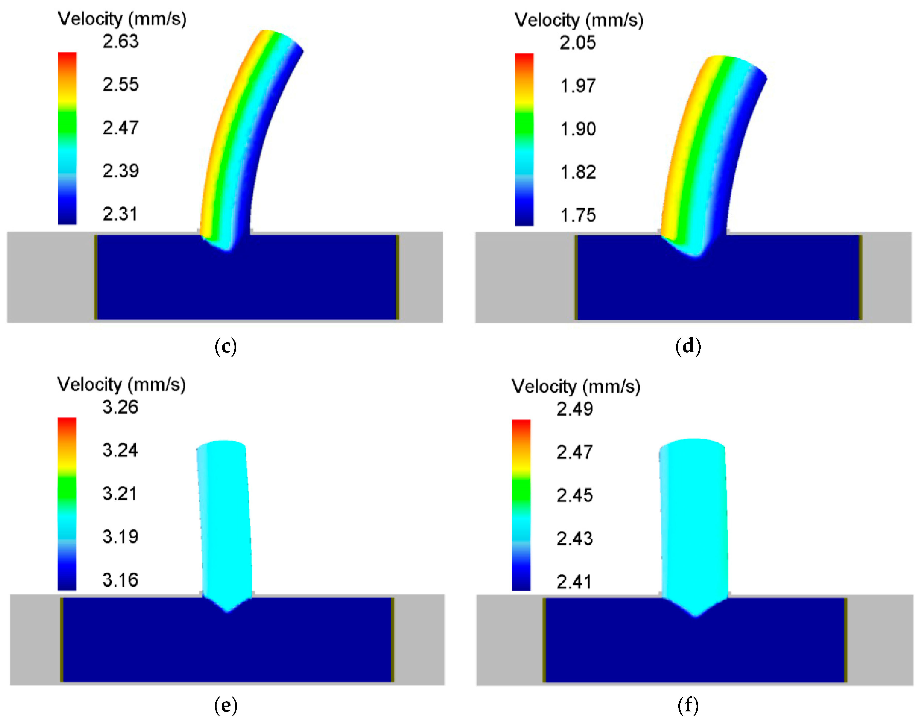
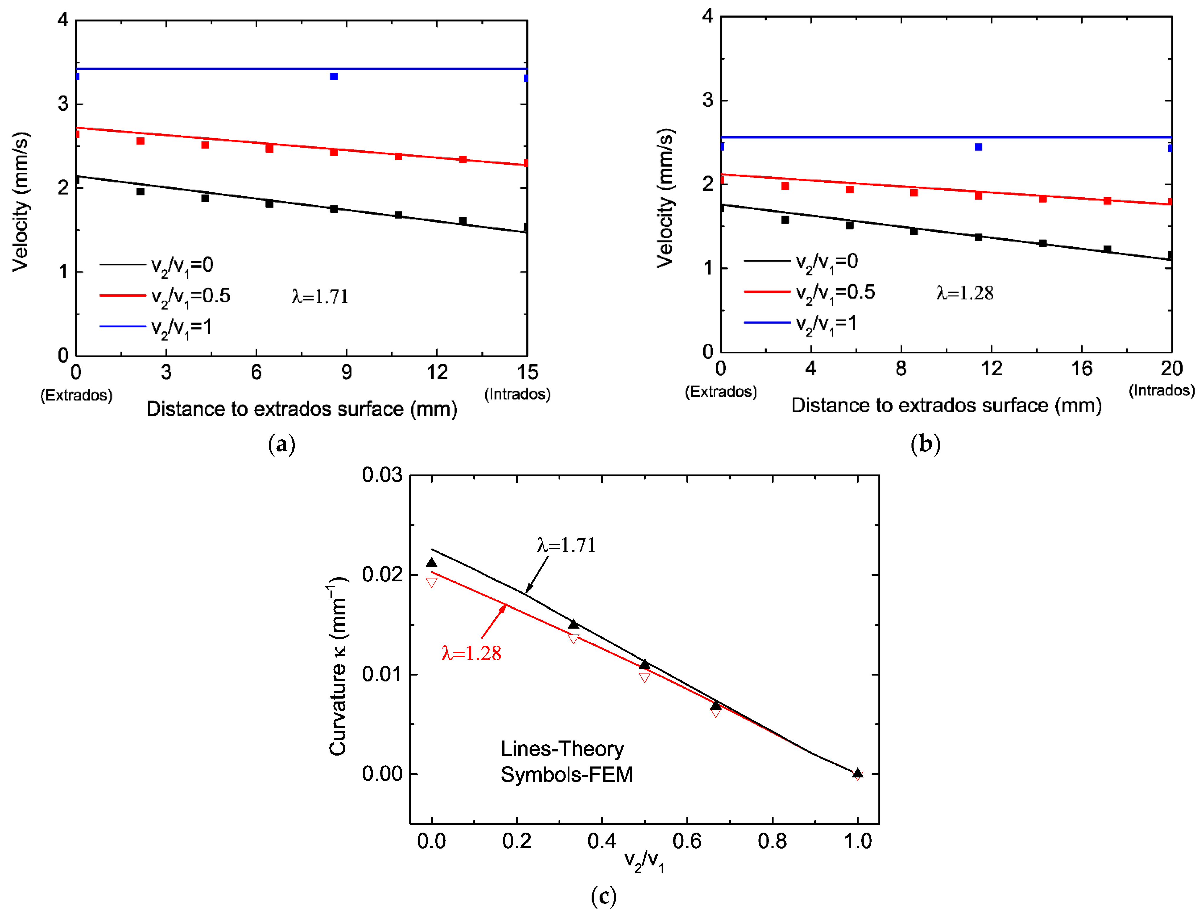
3.1. Prediction of the Extrudate Curvature

Figure 3 shows the simulated flow lines (~1.5 mm interval, at room temperature) of the billet and extrudate at different extrusion ratios and velocity ratios, from which the values of the eccentricity ratio variable ξ are extracted by manually drawing a line dividing the PDZ. The obtained values of ξ are shown in Figure 4, and the results predicted by the analytical model with different values of n are also plotted for comparison. As can be seen in Figure 4, a reasonably good agreement between the analytical results and FE modelling is achieved. It can also be seen that the eccentricity ratio variable ξ is hardly affected by the value of n; therefore, the n value is expected to have very little effect on the extrudate curvature, which will be discussed later. The asymmetrical patterns of the flow lines in Figure 3a–c clearly reflect that asymmetrical material flow caused by the differential extrusion velocities of upper and lower rams occurs at the die orifice. The interval (dense extent) of the flow lines in the extrudate also suggests the level of effective strain accumulated during the DVSE process. The quantitative comparison of the effective strain is discussed in Section 3.3.
Figure 5 shows the simulated material flow velocity distribution at the die exit orifice, which is compared with that obtained from the theoretical model in Figure 6a,b. As shown in Figure 5, an obvious velocity gradient across the die orifice exists for profiles extruded at a velocity ratio v2/v1 < 1. As a result, the profiles are bent towards the side which has a relatively lower velocity v2. In addition, it can be seen that the higher the velocity ratio v2/v1, the lower the extrudate curvature. The reason is that the velocity gradient across the die orifice decreases as the velocity ratio v2/v1 increases. It is noted that the velocity gradient for the cases of v2/v1 = 1, λ = 1.71 and v2/v1 = 1, λ = 1.28 are both negligible, although they are not exactly zero, possibly due to numerical errors. The specific value of the extrudate curvature obtained from FE modelling is shown in Figure 6c, which is estimated following procedures in previous works [32]. The curvature predicted from the theoretical model is also plotted for comparison.
We can see from Figure 6 that the predicted velocity and curvature by the theoretical model are generally compatible with the FE modelling results, and the curvature obtained from FE modelling is slightly smaller possibly due to the effect of friction at the die land on the material flow velocity at the die exit orifice, which was not considered in the theoretical model due to the very short die land length (2 mm). However, it might still have a straightening effect, and this straightening effect increases with the increase of the die land length [49]. As shown in Figure 6, FE modelling leads to a slightly reduced velocity gradient and thus smaller curvature of the extrudate compared with that obtained from theoretical analysis. It can also be seen that the n value has a negligible effect on the material flow velocity over the die exit orifice since it hardly affects the eccentricity ratio variable ξ ; therefore, the n value has a negligible effect on the extrudate curvature.

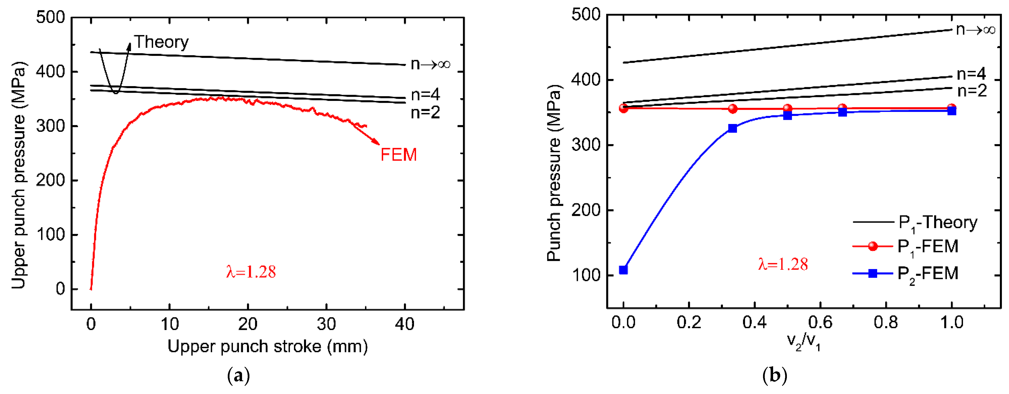
3.2. Prediction of the Extrusion Pressure

The extrusion pressure versus stroke obtained from FE modelling at velocity ratio v 2 / v 1 = 0 and extrusion ratio λ = 1.28 is shown in Figure 7a. The theoretical results obtained from different values of n are also plotted. It can be seen that the theoretically predicted extrusion pressure is higher than that obtained from FE modelling. The difference gradually decreases as the value of n decreases, and the minimum value of n = 2 gives the closest result. This is within expectations of the upper bound theory. Since the theoretically predicted value is always higher, the minimum value of the upper bound solution given by n = 2 will result in the best approximated extrusion pressure. As extrusion proceeds, the extrusion pressure gradually decreases as a result of decreased frictional surface area in the container. Figure 7b compares the extrusion pressure vs. velocity ratio obtained from theoretical analysis and FE modelling for velocity ratios v 2 / v 1 = 0 ~ 1 and an extrusion ratio λ = 1.28 . The stroke value used in the analytical model was the same as that in FE modelling, which was the stroke when the simulated pressure P 1 reaches peak value. The extrusion pressure P 2 of the lower ram was also extracted at this extrusion moment. Again, it can be seen that the theoretically predicted value is always higher than that obtained from FE modelling; the difference gradually decreases as the value of n decreases, and the minimum value of n = 2 gives the closest result. When v 1 > v 2 , the upper ram reaches the peak extrusion pressure earlier than that of the lower ram, which is reflected in the figure where the extrusion pressure P 2 is lower than   P 1 for v 2 / v 1 < 1 . The pressure difference of the two rams gradually decreases as their velocity difference decreases, and the greatest decrement in the extrusion pressure difference occurs at the very early stage of the velocity ratio increment, since the extrusion pressure of the lower ram is much lower when it is still than when it is moved, even at a very small velocity.

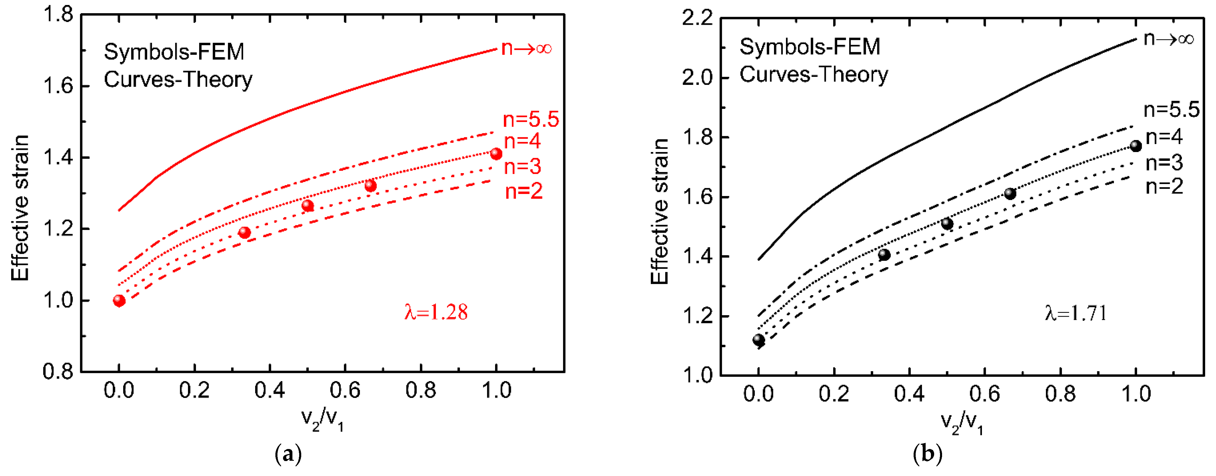
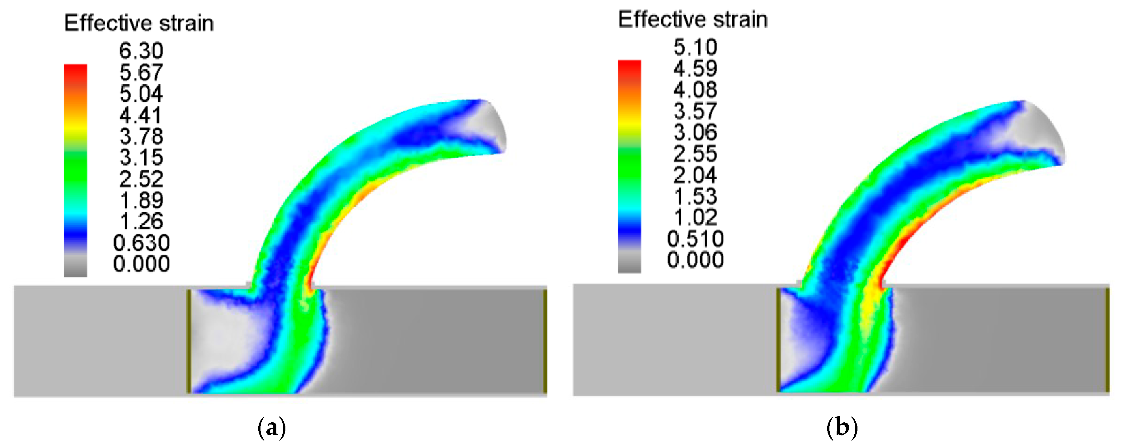
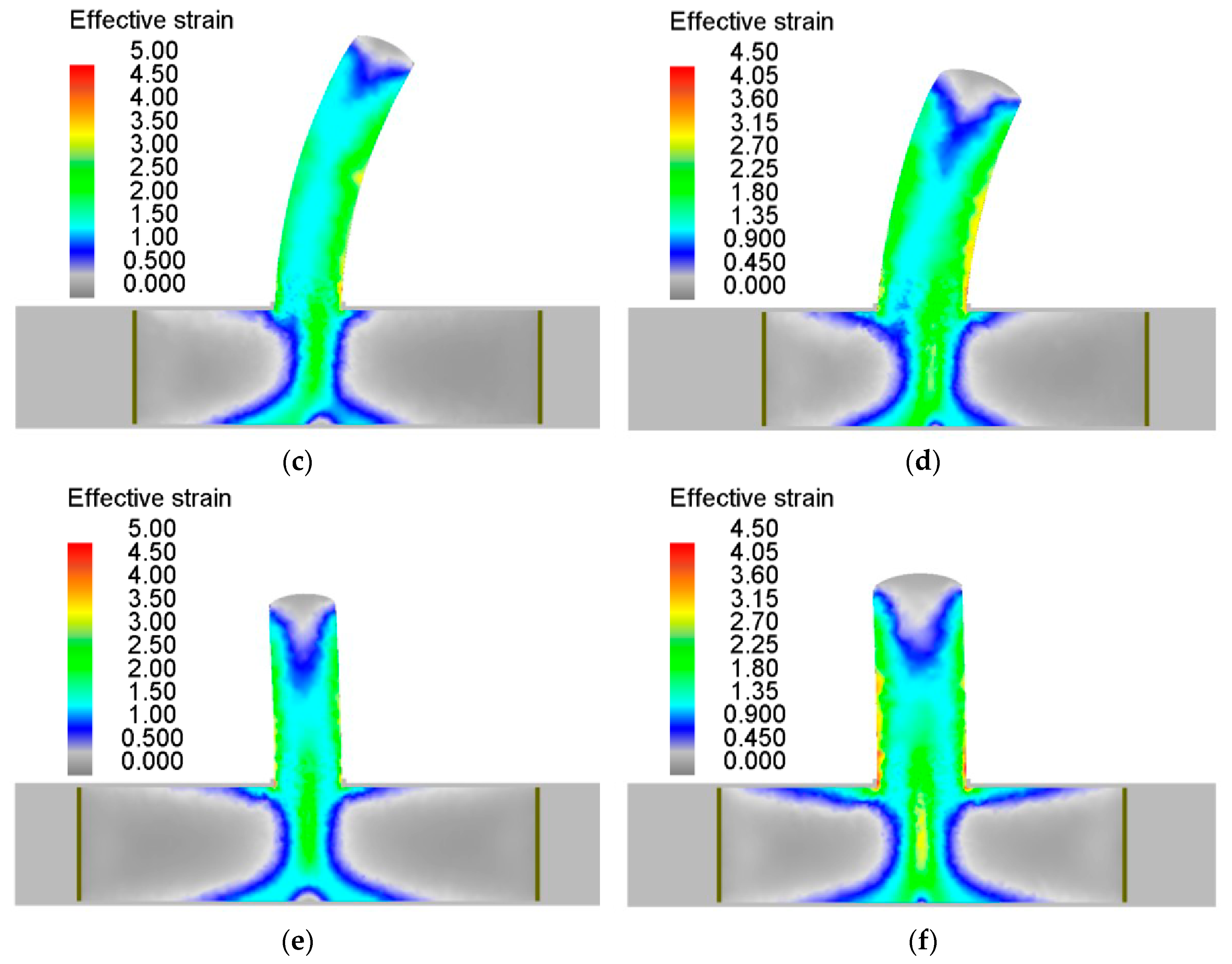
3.3. Prediction of the Effective Strain

The effective strain of the extrudate obtained from FE modelling [50] at different extrusion ratios and velocity ratios is shown in Figure 8. The average value of the effective strain over the cross-section of the outside bending part ( ξ c ) of the extrudate at the die orifice is extracted from FE modelling and compared with that predicted by the theoretical model with different values of n in Figure 9. It can be seen from Figure 9 that the predicted effective strain by the theoretical model increases as the value of n increases, and the limiting case ( n ) gives the upper limit value of the effective strain. For a given extrusion ratio, the n value for best predicting the effective strain is slightly increased as the velocity ratio v 2 / v 1 increases. As discussed before, the eccentricity ratio variable ξ decreases as the extrusion velocity ratio v 2 / v 1 increases; thus, the effective width ( ξ c ) of the extrusion exit channel decreases, leading to an increased effective extrusion reduction ratio ( p / ξ c ) and thus effective strain.
Figure 9 also shows that the best approximated effective strain on the whole is obtained for the case of n = 3.5. This value is slightly greater than the value of n = 2 for the best approximated extrusion pressure. As explained before, due to the essence of the upper bound theorem, the theoretically predicted extrusion pressure is always higher and decreases as the value of n decreases; thus, the value of n = 2 is simply determined because it gives the minimum theoretical result. The effective strain is inhomogeneous across the cross-section of the extrudate, suggesting that the n value might change slightly with positions for a given extrusion ratio and velocity ratio. In this work, the n value is considered to be constant for flow lines at different positions to study the mean effective strain; thus, a best fit value of n = 3.5 is obtained by comparing the theoretical and numerical results for different velocity ratios. To enable the prediction of the inhomogeneous effective strain distribution across the cross-section of the extrudate, the effect of the position on the value of n will be considered in the future. It should be noted that to avoid the velocity discontinuity, a fan-shaped flow line model in which any point of the material flows on a specific streamline having a unique trajectory of an ellipse has been proposed before. Although there is no velocity discontinuity in the PDZ where the material undergoes gradual and continuous change in velocity, the effective strain in the unique ellipse-shaped flow line model is not easily available, which can only be obtained numerically [50]. Here a more general form of the continuous flow line model is proposed, in which the flow line is more flexible depending on the shape parameter n. In addition, an explicit analytical expression of the effective strain can be derived (Equation (7)), which incorporates the upper limit obtained by the traditional discontinuous simple shear model [42,47] and provides a more easily available and accurate estimation. For n , Equation (7) results in ε ¯ m = p ξ c + ξ c p / 3 , which is the same as given by the simple shear model used before to estimate the extrudate effective strain.

4. Conclusions

A general flow line model controlled by the shape factor n has been presented on the basis of the upper bound theorem to better analytically describe the room temperature bending behaviour of AA1050 aluminium alloy profiles in a novel extrusion process: the differential velocity sideways extrusion (DVSE). It was concluded that the n value has a negligible effect on the material flow eccentricity ratio variable ξ of the AA1050 profiles in DVSE, and the minimum value of n = 2 gives the minimum and closest theoretical extrusion pressure. Additionally, the n value has a negligible effect on the material flow velocity over the die exit orifice and extrudate curvature since it hardly affects the eccentricity ratio variable ξ . The theoretically predicted velocity gradient is slightly greater than that obtained from FE modelling due to the straightening effect of the die bearing land being not considered; thus, the theoretically predicted curvature is slightly greater. For a given extrusion ratio, the n value for obtaining the best match average effective strain of the extrudate increases as the velocity ratio v 2 / v 1 increases, and the value of n = 3.5 results in the closest average effective strain as a whole.

Author Contributions

W.Z.—Investigation, Methodology, Data curation, Formal analysis, Writing—original draft, Writing—review & editing; Z.X.—Investigation, Software, Writing—review & editing. All authors have read and agreed to the published version of the manuscript.

Funding

This research received no external funding.

Institutional Review Board Statement

Not applicable.

Informed Consent Statement

Not applicable.

Data Availability Statement

The data presented in this study are available on request from the corresponding author.

Conflicts of Interest

The authors declare no conflict of interest.

Appendix A. Determination of the Velocity Field, Strain Rate and Effective Strain

An admissible velocity field satisfying the continuity equation can be defined as follows:
v x = q ψ y = y n 1 ξ c n n q
v y = q ψ x = x n 1 p n n q
where q is a parameter determined by the incoming velocity v 1 ( v 1 > 0 )   assumed to be the same at the incoming flow position   x 0 , i.e., at the plane defined by y = 0 . When x = x 0 ,   v y = v 1 then one obtains:
q = x 0 1 n p n v 1 n
When substituting Equation (A3) into Equations (A1) and (A2), the velocity field is then given by Equations (3) and (4).
The strain rate tensor can be obtained as:
ε ˙ x x = v x x = n 1 p ξ c n x 0 1 2 n x y n 1 v 1
ε ˙ y y = v y y = 1 n p ξ c n x 0 1 2 n x y n 1 v 1
ε ˙ x y = 1 2 v x y + v y x = 1 2 n 1 x 0 1 2 n p n x n 2 y ξ c n y n 2 x ξ c n v 1
When substituting Equations (A4)–(A6) into Equation (5), the effective strain rate can be obtained.
To obtain the effective strain, the following variable substitutions are made:
x p n = r n c o s 2 β
y ξ c n = r n s i n 2 β
x 0 p n = r n
where 0 β π 2 ,   0 r 1 , then:
x = p r c o s 2 n β
y = ξ c r s i n 2 n β
v x = p ξ c s i n 2 2 n β v 1
v y = c o s 2 2 n β v 1
When substituting Equations (A10) and (A11) into Equation (5), the effective strain rate is expressed as:
ε ˙ ¯ r , β = n 1 s i n β c o s β 2 4 n 3 r 1 p s i n 4 n β + p ξ c 2 c o s 4 n β v 1
The differential area element d x d y is:
d x d y = J r , β d r d β
where J r , β is the Jacobian determinant given by:
J r , β = x r x β y r y β
Substituting Equations (A10) and (A11) into Equation (A16) yields:
J r , β = 2 ξ c p r n s i n β c o s β 2 n 1
Thus:
P D Z ε ˙ ¯ x , y d x d y = 0 π 2 0 1 ε ˙ ¯ r , β J r , β d r d β = 0 π 2 2 n 1 v 1 3 n ( ξ c s i n 1 + 2 n β c o s 1 2 n β + p 2 ξ c s i n 1 2 n β c o s 1 + 2 n β ) d β = π n 1 ξ c + p 2 ξ c v 1 3 n 2 sin π n
P D Z d x d y = 0 π 2 0 1 J r , β d r d β = 0 π 2 ξ c p n s i n β c o s β 2 n 1 d β = ξ c p B 1 n , 1 n 2 n
ε ˙ ¯ m = P D Z ε ˙ ¯ x , y d x d y P D Z d x d y = 2 π n 1 1 p + p ξ c 2 v 1 3 n s i n π n B 1 n , 1 n
Based on the volume constancy, to replace the material in the PDZ with the material in the entrance channel, a ram stroke needed is:
Δ l 1 = P D Z d x d y p = ξ c B 1 n , 1 n   2 n
The deformation time t is calculated by the time needed for producing the stroke Δ l 1 :
t = Δ l 1 v 1 = ξ c B 1 n , 1 n   2 n v 1  
When substituting Equations (A20) and (A22) into Equation (7), the effective strain can be obtained.

Appendix B. Determination of the Internal Power Dissipation

Using Equation (A17), the differential volume element in the PDZ can be obtained as:
d V = w d x d y = w J r , β d r d β = 2 w ξ c p r n s i n β c o s β 2 n 1 d r d β
Thus:
W ˙ d e f = 3 0 π 2 0 1 k ¯ ε ˙ ¯ r , β w J r , β d r d β = 2 0 π 2 k ¯ w n 1 v 1 n ( ξ c s i n 1 + 2 n β c o s 1 2 n β + p 2 ξ c s i n 1 2 n β c o s 1 + 2 n β ) d β = k ¯ w p 2 + ξ c 2 π n 1 v 1 ξ c n 2 sin π n
d l in Equation (9) is the differential length element on the DMZ boundary and can be obtained when Equations (A10) and (A11) are applied with r = 1 :
d l = d x 2 + d y 2 = 2 n p 2 s i n 2 β c o s 4 n 2 β + ξ c 2 s i n 4 n 2 β c o s 2 β d β
Taking into account Equations (A12) and (A13), the related velocity discontinuity variable is:
Δ v = v x 2 + v y 2 = p 2 ξ c 2 s i n 4 4 n β + c o s 4 4 n β v 1
Thus:
W ˙ S v = 2 0 π 2   k ¯ w v 1 n p 2 ξ c sin 3 2 n β c o s 2 n 1 β + ξ c s i n 2 n 1 β c o s 3 2 n β d β = k ¯ w p 2 + ξ c 2 B 1 n , 2 1 n v 1 ξ c n

Appendix C. Determination of the Extrudate Curvature

As shown in Figure 2, assume the material at points O 3 , O 4 moves Δ X 3 , Δ X 4 , respectively, after a finite time element Δ t . As Δ X 3 > Δ X 4 , the extrudate will have a bending radius R , and the kinematic relations are:
Δ X 3 = v 3 Δ t  
Δ X 4 = v 4 Δ t  
The following geometrical relations exist:
Δ X 3 Δ X 4 = R Y ¯ 3 R Y ¯ 4  
where Y ¯ 3 , Y ¯ 4 are the Y-coordinates of the centres of volume of the two prisms, respectively:
Y ¯ 3 = V Y d V 3 V 3 = S 3 Y v X d S 3 S 3 v 3  
Y ¯ 4 = V Y d V 4 V 4 = S 4 Y v X d S 4 S 4 v 4  
where V 3 , V 4 are the volumes of the two prisms and d S 3 , d S 4 are the related differential surface elements. When substituting Equations (A28) and (A29) into Equation (A30), the bending radius R and curvature κ of the extrudate can be determined as Equations (17) and (18).
According to the principle of mass conservation:
v o = p c v 1 + v 2 = λ v 1 + v 2
v X is expressed in terms of Y ¯ 3   as:
v X = v 3 v o Y ¯ 3 Y + v o
When substituting Equations (A33) and (A34) into Equation (A31), Y ¯ 3 can be calculated as:
Y ¯ 3 = S 3 Y v X d S 3 S 3 v 3 = c 2 ξ 1 2 c Y v 3 v o Y ¯ 3 Y + v o w d Y ξ c w v 3 = ξ 1 2 3 + 1 8 c 2 ( v 3 v o ) 3 ξ Y ¯ 3 v 3 ξ ξ 2 c v o 2 ξ v 3
Equation (A35) is a quadratic equation of Y ¯ 3 where the negative root is the value needed for Y ¯ 3 :
Y ¯ 3 2 + ξ ξ 2 c v o 2 ξ v 3 Y ¯ 3 ξ 1 2 3 + 1 8 c 2 ( v 3 v o ) 3 ξ v 3 = 0  
Y ¯ 4 can be calculated similarly. Then v 1 e and v 2 e can be obtained by substituting Y = 1 2 c and 1 2 c into Equation (A34), respectively.

References

  1. Allwood, J.M.; Dunant, C.F.; Lupton, R.C.; Cleaver, C.J.; Serrenho, A.C.H.; Azevedo, J.M.C.; Horton, P.M.; Clare, A.; Low, H.; Horrocks, I.; et al. Absolute zero: Delivering the UK’s climate change commitment with incremental changes to today’s technologies. UK FIRES 2019. [Google Scholar] [CrossRef]
  2. Joost, W.J. Reducing vehicle weight and improving U.S. energy efficiency using integrated computational materials engineering. JOM 2012, 64, 1032–1038. [Google Scholar] [CrossRef] [Green Version]
  3. Hirsch, J. Recent development in aluminium for automotive applications. Trans. Nonferr. Met. Soc. China 2014, 24, 1995–2002. [Google Scholar] [CrossRef]
  4. Kohar, C.P.; Zhumagulov, A.; Brahme, A.; Worswick, M.J.; Mishra, R.K.; Inal, K. Development of high crush efficient, extrudable aluminium front rails for vehicle lightweighting. Int. J. Impact Eng. 2016, 95, 17–34. [Google Scholar] [CrossRef]
  5. Zhou, W.; Shao, Z.; Yu, J.; Lin, J. Advances and trends in forming curved extrusion profiles. Materials 2021, 14, 1603. [Google Scholar] [CrossRef]
  6. Chatti, S.; Dirksen, U.; Schikorra, M.; Kleiner, M. System for design and computation of lightweight structures made of bent profiles. Adv. Mater. Res. 2005, 6, 279–286. [Google Scholar] [CrossRef]
  7. Chatti, S. Production of Profiles for Lightweight Structures; Books on Demand GmbH: Norderstedt, Germany, 2005. [Google Scholar]
  8. Stevenson, K. Aluminum Extrusion Manual, 4th ed.; Aluminum Extruders Council: Chicago, IL, USA, 2014. [Google Scholar]
  9. Tekkaya, A.E.; Chatti, S. Bending (Tubes, Profiles); Springer: Berlin/Heidelberg, Germany, 2014. [Google Scholar]
  10. Merklein, M.; Geiger, M. New materials and production technologies for innovative lightweight constructions. J. Mater. Process. Technol. 2002, 125, 532–536. [Google Scholar] [CrossRef]
  11. Kleiner, M.; Chatti, S.; Klaus, A. Metal forming techniques for lightweight construction. J. Mater. Process. Technol. 2006, 177, 2–7. [Google Scholar] [CrossRef]
  12. Tekkaya, A.E.; Khalifa, N.B.; Grzancic, G.; Hölker, R. Forming of lightweight metal components: Need for new technologies. Procedia Eng. 2014, 81, 28–37. [Google Scholar] [CrossRef] [Green Version]
  13. Vollertsen, F.; Sprenger, A.; Kraus, J.; Arnet, H. Extrusion, channel, and profile bending: A review. J. Mater. Process. Technol. 1999, 87, 1–27. [Google Scholar] [CrossRef]
  14. Yang, H.; Li, H.; Zhang, Z.; Zhan, M.; Liu, J.; Li, G. Advances and trends on tube bending forming technologies. Chin. J. Aeronaut. 2012, 25, 1–12. [Google Scholar] [CrossRef] [Green Version]
  15. Chatti, S.; Hermes, M.; Kleiner, M. Three-Dimensional Bending of Profiles by Stress Superposition; Springer: Berlin/Heidelberg, Germany, 2007. [Google Scholar]
  16. Hermes, M.; Staupendahl, D.; Kleiner, M. Torque Superposed Spatial Bending; Springer: Berlin/Heidelberg, Germany, 2015. [Google Scholar]
  17. Hermes, M.; Kleiner, M. Method and Device for Profile Bending. U.S. Patent 9,227,236, 5 January 2016. [Google Scholar]
  18. Hermes, M.; Kurze, S.; Tekkaya, A.E. Method and Device for Forming a Bar Stock. European Patent EP2203264B1, 27 April 2011. [Google Scholar]
  19. Chatti, S.; Hermes, M.; Weinrich, A.; Ben-Khalifa, N.; Tekkaya, A.E. New incremental methods for springback compensation by stress superposition. Int. J. Mater. Form. 2009, 2, 817–820. [Google Scholar] [CrossRef]
  20. Kleiner, M.; Tekkaya, A.E.; Chatti, S.; Hermes, M.; Weinrich, A.; Ben-Khalifa, N.; Dirksen, U. New incremental methods for springback compensation by stress superposition. Prod. Eng. 2009, 3, 137–144. [Google Scholar] [CrossRef]
  21. Becker, C.; Hermes, M.; Tekkaya, A.E. Incremental Tube Forming; Springer: Berlin/Heidelberg, Germany, 2015. [Google Scholar]
  22. Chatti, S.; Hermes, M.; Tekkaya, A.E.; Kleiner, M. The new TSS bending process: 3D bending of profiles with arbitrary cross-sections. CIRP Ann. 2010, 59, 315–318. [Google Scholar] [CrossRef] [Green Version]
  23. Kleiner, M.; Arendes, D. The manufacture of non-linear aluminium sections applying a combination of extrusion and curving. In Proceedings of the Fifth International Conference on Technology of Plasticity, Columbus, OH, USA, 7–10 October 1996; pp. 971–974. [Google Scholar]
  24. Selvaggio, A.; Becker, D.; Klaus, A.; Arendes, D.; Kleiner, M. Curved Profile Extrusion; Springer: Berlin/Heidelberg, Germany, 2015. [Google Scholar]
  25. Müller, K.B. Bending of extruded profiles during extrusion process. Mater. Forum 2004, 28, 264–269. [Google Scholar] [CrossRef]
  26. Müller, K.B. Bending of extruded profiles during extrusion process. Int. J. Mach. Tools Manuf. Mater. 2006, 46, 1238–1242. [Google Scholar] [CrossRef]
  27. Brosius, A.; Hermes, M.; Ben Khalifa, N.; Trompeter, M.; Tekkaya, A.E. Innovation by forming technology: Motivation for research. Int. J. Mater. Form. 2009, 2, 29–38. [Google Scholar] [CrossRef]
  28. Ben Khalifa, N.; Selvaggio, A.; Pietzka, D.; Haase, M.; Tekkaya, A.E. Advanced extrusion processes. Mater. Res. Innov. 2011, 15, 487–490. [Google Scholar] [CrossRef]
  29. Nikawa, M.; Shiraishi, M.; Miyajima, Y.; Horibe, H.; Goto, Y. Production of shaped tubes with various curvatures using extrusion process through inclined die aperture. J. Jpn. Soc. Technol. Plast. 2002, 43, 654–656. [Google Scholar]
  30. Shiraishi, M.; Nikawa, M.; Goto, Y. An investigation of the curvature of bars and tubes extruded through inclined dies. Int. J. Mach. Tools Manuf. 2003, 43, 1571–1578. [Google Scholar] [CrossRef]
  31. Takahashi, Y.; Kihara, S.; Yamaji, K.; Shiraishi, M. Effects of die dimensions for curvature extrusion of curved rectangular bars. Mater. Trans. 2015, 56, 844–849. [Google Scholar] [CrossRef] [Green Version]
  32. Zhou, W.; Lin, J.; Dean, T.A.; Wang, L. Feasibility studies of a novel extrusion process for curved profiles: Experimentation and modelling. Int. J. Mach. Tools Manuf. 2018, 126, 27–43. [Google Scholar] [CrossRef] [Green Version]
  33. Zhou, W.; Yu, J.; Lin, J.; Dean, T.A. Manufacturing a curved profile with fine grains and high strength by differential velocity sideways extrusion. Int. J. Mach. Tools Manuf. 2019, 140, 77–88. [Google Scholar] [CrossRef]
  34. Zhou, W.; Yu, J.; Lu, X.; Lin, J.; Dean, T.A. A comparative study on deformation mechanisms, microstructures and mechanical properties of wide thin-ribbed sections formed by sideways and forward extrusion. Int. J. Mach. Tools Manuf. 2021, 168, 103771. [Google Scholar] [CrossRef]
  35. Ghassemali, E.; Tan, M.-J.; Jarfors, A.E.W.; Lim, S.C.V. Optimization of axisymmetric open-die micro-forging/extrusion processes: An upper bound approach. Int. J. Mech. Sci. 2013, 71, 58–67. [Google Scholar] [CrossRef]
  36. Parvizi, A.; Abrinia, K. A two dimensional upper bound analysis of the ring rolling process with experimental and FEM verifications. Int. J. Mech. Sci. 2014, 79, 176–181. [Google Scholar] [CrossRef]
  37. Wu, Y.; Dong, X.; Yu, Q. Upper bound analysis of axial metal flow inhomogeneity in radial forging process. Int. J. Mech. Sci. 2015, 93, 102–110. [Google Scholar] [CrossRef]
  38. Zhang, X.J.; Li, F.; Wang, Y.; Chen, Z.Y. An analysis for magnesium alloy curvature products formed by staggered extrusion (SE) based on the upper bound method. Int. J. Adv. Manuf. Technol. 2021, 119, 303–313. [Google Scholar] [CrossRef]
  39. Farahmand, H.R.; Abrinia, K. An upper bound analysis for reshaping thick tubes to polygonal cross-section tubes through multistage roll forming process. Int. J. Mech. Sci. 2015, 100, 90–98. [Google Scholar] [CrossRef]
  40. Wu, Y.; Dong, X. An upper bound model with continuous velocity field for strain inhomogeneity analysis in radial forging process. Int. J. Mech. Sci. 2016, 115, 385–391. [Google Scholar] [CrossRef]
  41. Cai, S.-p.; Wang, Z.-j. An analysis for three-dimensional upset forging of elliptical disks and rings based on the upper-bound method. Int. J. Mech. Sci. 2020, 183, 105835. [Google Scholar] [CrossRef]
  42. Lee, D.N. An upper-bound solution of channel angular deformation. Scr. Mater. 2000, 43, 115–118. [Google Scholar] [CrossRef]
  43. Segal, V.M. Equal channel angular extrusion: From micromechanics to structure formation. Mater. Sci. Eng. A 1999, 271, 322–333. [Google Scholar] [CrossRef]
  44. Altan, B.S.; Purcek, G.; Miskioglu, I. An upper-bound analysis for equal-channel angular extrusion. J. Mater. Process. Technol. 2005, 168, 137–146. [Google Scholar] [CrossRef]
  45. Ebrahimi, R.; Reihanian, M.; Kanaani, M.; Moshksar, M.M. An upper-bound analysis of the tube extrusion process. J. Mater. Process. Technol. 2008, 199, 214–220. [Google Scholar] [CrossRef]
  46. Laptev, A.M.; Perig, A.V.; Vyal, O.Y. Analysis of equal channel angular extrusion by upper bound method and rigid blocks model. Mater. Res. 2013, 17, 359–366. [Google Scholar] [CrossRef] [Green Version]
  47. Zhou, W.; Lin, J.; Dean, T.A.; Wang, L. Analysis and modelling of a novel process for extruding curved metal alloy profiles. Int. J. Mech. Sci. 2018, 138, 524–536. [Google Scholar] [CrossRef]
  48. Kwan, C.-T.; Hsu, Y.-C. An analysis of pseudo equal-cross-section lateral extrusion through a curved channel. J. Mater. Process. Technol. 2002, 122, 260–265. [Google Scholar] [CrossRef]
  49. Zhou, W.; Yu, J.; Lin, J.; Dean, T.A. Effects of die land length and geometry on curvature and effective strain of profiles produced by a novel sideways extrusion process. J. Mater. Process. Technol. 2020, 282, 116682. [Google Scholar] [CrossRef]
  50. Zhou, W.; Shi, Z.; Lin, J. Upper bound analysis of differential velocity sideways extrusion process for curved profiles using a fan-shaped flow line model. Int. J. Lightweight Mater. Manuf. 2018, 1, 21–32. [Google Scholar] [CrossRef]
Figure 1. (a) Schematic of the differential velocity sideways extrusion (DVSE) process, (b) deformation model diagram of the DVSE process and (c) velocity hodograph of the developed flow line model for a point Q (x,y) on a flow line entering at an arbitrary location x = x 0 .
Metals 12 00877 g001
Figure 2. Schematic of the velocity gradient across the die orifice and the bending radius, using the local Cartesian coordinate system O-XYZ.
Metals 12 00877 g002
Figure 3. Material flow lines at different extrusion ratios and velocity ratios: (a) λ = 1.28, v2/v1 = 0, (b) λ = 1.71, v2/v1 = 0, (c) λ = 1.71, v2/v1 = 0.5 and (d) λ = 1.71, v2/v1 = 1.
Metals 12 00877 g003
Figure 4. Comparison of the analytical and simulated eccentricity ratio ξ at different velocity ratios and extrusion ratios (room temperature).
Metals 12 00877 g004
Figure 5. Simulated material flow velocity distribution at different extrusion ratios and velocity ratios, highlighting the velocity gradient of the extruded profile across the die orifice: (a) v2/v1 = 0, λ = 1.71, (b) v2/v1 = 0, λ = 1.28, (c) v2/v1 = 0.5, λ = 1.71, (d) v2/v1 = 0.5, λ = 1.28, (e) v2/v1 = 1, λ = 1.71 and (f) v2/v1 = 1, λ = 1.28.
Metals 12 00877 g005aMetals 12 00877 g005b
Figure 6. Material flow velocity across the die orifice and extrudate curvature obtained from theory (lines) at different n values, and comparison of those extracted from FEM (symbols): (a) velocity, λ = 1.71, (b) velocity, λ = 1.28 and (c) curvature.
Metals 12 00877 g006
Figure 7. Extrusion pressure P 1 of the upper ram obtained from theory at different n values, and comparison of those extracted from FEM: (a) P 1 vs. stroke at v2/v1 = 0, λ = 1.28 and (b) P 1 vs. velocity ratio at v2/v1 = 0~1 and λ = 1.28.
Metals 12 00877 g007
Figure 8. Simulated effective strain distribution at different extrusion ratios and velocity ratios: (a) v2/v1 = 0, λ = 1.71, (b) v2/v1 = 0, λ = 1.28, (c) v2/v1 = 0.5, λ = 1.71, (d) v2/v1 = 0.5, λ = 1.28, (e) v2/v1 = 1, λ = 1.71 and (f) v2/v1 = 1, λ = 1.28.
Metals 12 00877 g008aMetals 12 00877 g008b
Figure 9. Effective strain of the extrudate obtained from theory (lines) at different n values, and comparison of those extracted from FEM (symbols): (a) λ = 1.28, v2/v1 = 0~1 and (b) λ = 1.71, v2/v1 = 0~1.
Metals 12 00877 g009
Publisher’s Note: MDPI stays neutral with regard to jurisdictional claims in published maps and institutional affiliations.

