Article

Machine-Learning-Based Model of Elastic—Plastic Deformation of Copper for Application to Shock Wave Problem

by
Alexander E. Mayer
*,
Mikhail V. Lekanov
,
Natalya A. Grachyova
and
Eugeniy V. Fomin
Department of Physics, Chelyabinsk State University, 454001 Chelyabinsk, Russia
*
Author to whom correspondence should be addressed.
Metals 2022, 12(3), 402; https://doi.org/10.3390/met12030402
Submission received: 10 January 2022 / Revised: 21 February 2022 / Accepted: 23 February 2022 / Published: 25 February 2022
(This article belongs to the Special Issue Shock-Wave Loading of Metallic Materials)

Abstract

:
Molecular dynamics (MD) simulations explored the deformation behavior of copper single crystal under various axisymmetric loading paths. The obtained MD dataset was used for the development of a machine-learning-based model of elastic–plastic deformation of copper. Artificial neural networks (ANNs) approximated the elastic stress–strain relation in the form of tensor equation of state, as well as the thresholds of homogeneous nucleation of dislocations, phase transition and the beginning of spall fracture. The plastic part of the MD curves was used to calibrate the dislocation plasticity model by means of the probabilistic Bayesian algorithm. The developed constitutive model of elastic–plastic behavior can be applied to simulate the shock waves in thin copper samples under dynamic impact.

1. Introduction

The structure and evolution of shock waves in pure metals [1,2,3,4,5], alloys [6] and microstructured material [7,8,9,10] still attract an increased attention, due to both the fundamental interest in dynamic behavior of materials and the practical issues related to high-energy-density technologies, aerospace and defense applications. The structure and evolution are closely related with plasticity, phase transformations and other processes of defect formation, as well as with the response of the existing microstructure of material. Even in the case of pure metals, the material response on the dynamic loading is complex and not completely explored [2,3], especially in the transient modes [11]. The application of short [12,13] and ultra-short powerful laser pulses for the irradiation of thin metal samples expands the range of strain rates investigated in experiments up to 107–109 s–1 [14,15,16,17]. These strain rates can be realized in molecular dynamics (MD) simulations for representative volume elements, but direct MD simulation of the shock-wave processes [18,19,20] is restricted from bellow by much higher strain rates—typically of about 1011 s–1. Thus, continuum mechanics models are used to investigate the shock-wave problem numerically [21,22,23,24]. It makes essential a transfer of information from the MD, which allows one to study the rich physics of inelastic deformation, to continuum models applicable for realistic spatial and temporal scales.
There are a large number of MD researches of elementary processes of the inelastic behavior of materials; the MD is used to determine parameters required on the level of crystal plasticity or continuum model. One can mention the investigations of the motion of dislocations [25,26,27], their interaction with precipitates in alloys [28,29,30] and many other problems. For instance, MD simulations of pure Cu and Cu-Ni solid solution are used in Reference [27] to fit the parameters of dislocation motion equation, which is further used in 2D discrete dislocation dynamics to describe the relaxation properties of an ensemble of dislocations. MD data on the interaction of an edge dislocation with θ’ precipitate in Al are applied in Reference [30] to fit the parameters of the dislocation–precipitate interaction model; in turn, this model is used in the frames of 2D discrete dislocation dynamics to investigate, at the macro-level, the flow strength of the alloy and its degradation due to successive cutting of precipitates. At the same time, the machine-learning techniques are intensively developing for applications in material science [31,32,33]. In application to the considered problem, they pave the way for automated and more accurate data transfer from the MD based on a series of MD runs and probability-based algorithms [34].
In the present paper, we propose a new approach to the data transfer from the MD to continuum model by application of machine-learning-based methods, which use the datasets generated by means of MD simulations. Unambiguous state functions, such as the elastic stress–strain relation and the dislocation nucleation threshold at a certain strain rate are approximated by artificial neural networks (ANNs). The kinetic process of plasticity is described by the time-differential equations of the dislocation plasticity model, and the machine-learning-type Bayesian algorithm is used to fit model parameters on the basis of MD data. Here we considerably develop our previous research [34], in which application of the ANNs was proposed to the tensor equation of state and nucleation threshold. In the present paper, we add the Bayesian calibration of the plasticity model that makes complete the data transfer from the MD to the continuum model, including the inelastic stage of deformation. As compared with Reference [34], we use a more accurate description of the dislocation nucleation by means of the strain-distance function introduced in Reference [35] and take into account the strain-rate dependence of the dislocation nucleation. The same methodology is applied to the void nucleation and phase transition. As compared with Reference [34], a wider range of strain paths is considered, including a combination of simultaneous tension and compression along different axes, and a more detailed analysis of the obtained MD data is performed.
We apply our approach to the case of copper single crystal as an example of material extensively investigated by means of MD simulations in recent years [36,37,38]. Section 2 describes the applied methods, including MD simulations of the deformation of a representative volume element along various deformation paths, its processing and incorporation into the constitutive model. Section 3 presents the results of application of this methodology to the case of the single copper crystal. We consider axisymmetric deformation, because it is related with the loading by a plane shock wave. Section 4 and Section 5 discuss and conclude the obtained results.

2. Materials and Methods

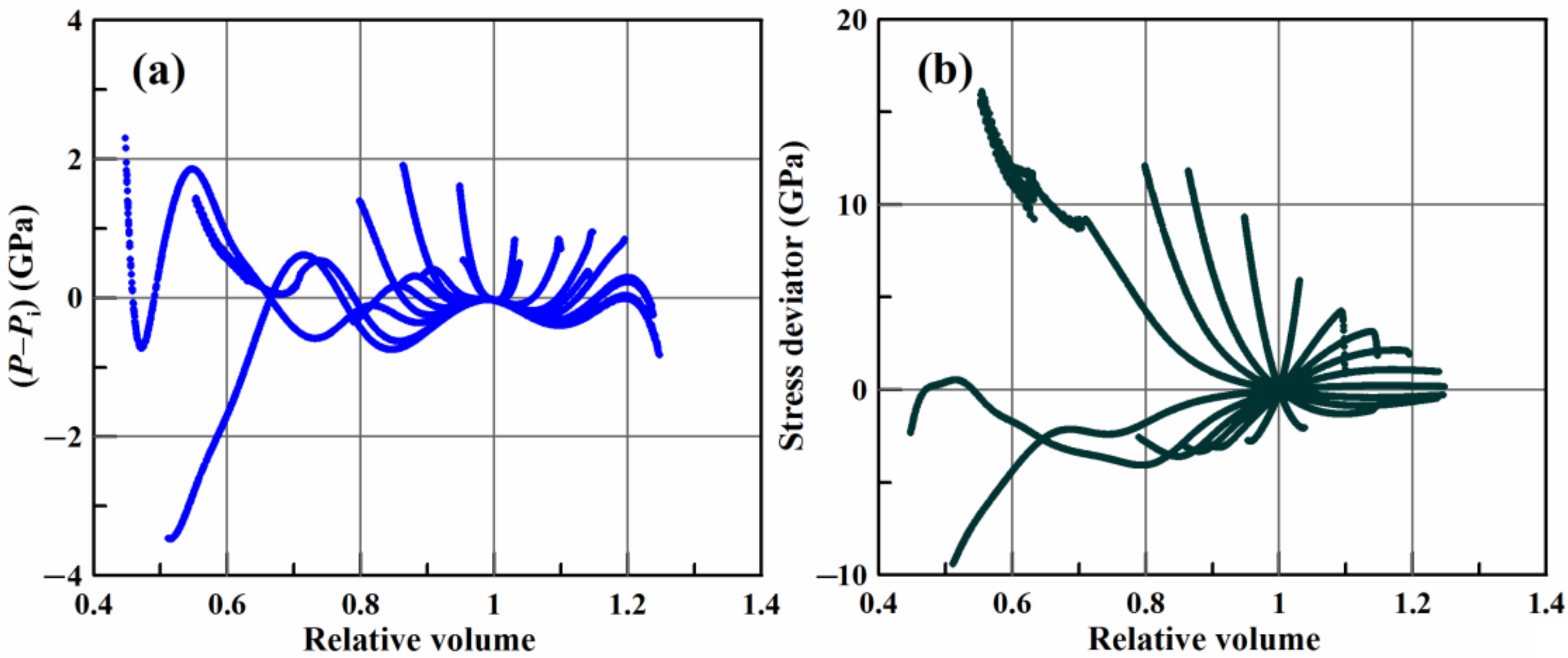
2.1. MD Simulations of Uniform Axisymmetric Deformation

MD simulations performed by means of LAMMPS software package [39], version 12Dec18, with EAM-type potential for Cu atoms [40] were used to explore the deformation behavior of copper single crystal under axisymmetric deformation. Different deformation paths were considered and are presented in Table 1, with the axial engineering strain rate ( ε ˙ x ) and the transverse engineering strain rate ( ε ˙ y = ε ˙ z ) fulfilling the following requirement: ε ˙ 0 = ε ˙ x + 2 ε ˙ y = 1 ns 1 . In the case of simultaneous tension or compression along all axes ε ˙ x ε ˙ y 0 , the strain rate ( ε ˙ 0 ) coincides with the absolute value of the volumetric strain rate, while in the case of combination of tension and compression along different axes, ε ˙ x ε ˙ y < 0 , the used strain rate ( ε ˙ 0 ) is a more convenient measure than the volumetric strain rate. For instance, if ε ˙ x = ε ˙ y / 2 , the volumetric strain rate is zero, while the deformation takes place, and the value ε ˙ 0 characterizes its rate.
The axis of symmetry, x , coincides with the lattice direction [100]. Uniform deformation is applied by means of the “fix deform” command, which rescales the atom coordinates. Initially, the MD system is cubic, and the edge length at 300 K is equal to L 0 = 18.16 nm ; half a million atoms is arranged in fcc lattice. The deformation transforms the sample into a parallelepiped with the edge lengths equal to L x along the axis of symmetry and L y = L z along the perpendicular directions. The diagonal components of the Cauchy–Green tensor can be expressed as follows [41]:
E 11 = 1 2 L x L 0 2 1 = ε x + 1 2 ε x 2 ,   E 22 = 1 2 L y L 0 2 1 = ε y + 1 2 ε y 2 ,
while the non-diagonal components are zero. The second parts of these equalities (expression through ε x and ε y ) are valid only for 300 K. The constant temperature is supported by Nose–Hoover thermostat [42] during the deformation. We consider the temperatures starting from 100 K up to 1300 K with the step of 100 K. Preliminary thermalization for 10 ps at zero pressure and test temperature is adopted before the deformation.
The investigated deformation paths form a dense grid of deformed states in the space E 11 , E 22 ; see Figure 1a. We do not consider pure hydrostatic (volumetric) tension/compression, but the path DG0 is close to it. The paths DG0–DG5 involve either tension or compression, while the paths DG6–DG9 combine axial compression with transverse tension and vice versa.
The points plotted in Figure 1 correspond to the elastic part of the deformation paths until the nucleation of dislocations or voids. The set of elastic compressive deformed states is elongated along the hydrostatic compression path, which is a diagonal in the coordinates E 11 , E 22 (Figure 1a). This is because the shear stress growths relatively slow during the increase in pressure along these paths, while an increase in pressure raises the threshold of dislocation nucleation [35,43,44]. Thus, we do not detect a transition to plastic deformation for the case of DG0 deformation path, and the entire calculated compressive part of this deformation path is shown. The transition to the coordinates of the relative volume is as follows:
V V 0 E V = 2 E 11 + 1 2 E 22 + 1 2 ,
where V is the current specific volume, and V 0 is the initial specific volume; and the shear strain,
E S E 11 E 22 / 2   ,
makes the distribution of the elastic states fitted in a rectangular domain (Figure 1b), which is more convenient for subsequent approximation of MD data by an ANN.
The incipience of plasticity and fracture during the deformation is detected by using the analysis of pressure, shear stress and temperature curves in combination with the analysis of atomic configurations. The onset of plasticity leads to a sharp drop in shear stress and a temperature spike: the thermostat cannot absorb all the energy released by the plastic flow. The beginning of tensile fracture leads to an abrupt increase in pressure and a strong temperature spike, due to the formation and growth of voids. Bursts in a monotonous evolution of the total energy can also be used as signs of inelastic behavior.
Concerning the atomic configurations, the transition to inelastic deformation is well seen with the help of “Polyhedral template matching” algorithm [45], which identifies different crystal structures: an emergence of hcp phase indicates the stacking faults, which are the traces of partial Shockley dislocations typical for copper and other fcc metals. The same algorithm identifies a complete or partial transition into bcc structure in most cases of deformation prior to the dislocation nucleation. This phase transition is not an inelastic process, because it does not lead to the energy dissipation and temperature spike. Detection of dislocations by means of DXA algorithm [46] and detection of voids by means of “Construct surface mesh” algorithm [47] are also used. All of these algorithms are realized in the OVITO program [48].
The virial theorem is used for the calculation of stresses, which are equivalent to the Cauchy stresses, σ , of continuum mechanics [49].

2.2. Training of ANNs for Tensor Equation of State and Structural Transformations

At first, consider the preparation of the training dataset for the tensor equation of state (EOS) in the form of artificial neural network (ANN). This EOS takes into account the nonlinear dependence of both pressure, P = σ 11 + 2 σ 22 / 3 , and stress deviator, S σ 11 + P , on the strains characterized by two quantities, E V and E S .
Figure 2 shows the room-temperature isotherm of copper as a compilation of the curves for all the deformation paths DG0–DG9. Our data are in good agreement with the experiments [50] involving diamond anvil cell and DFT calculations [51]; see Figure 2a. This agreement verifies the used interatomic potential [40]. According to the previous literature [35,44] and present MD results, the shear deformation affects the pressure, but this influence is much weaker than the influence of density (volume) variation. Therefore, the difference in pressure between the deformation paths is not seen on this scale. It is difficult for the ANN to describe such small variations against the background of a strong main trend of pressure increase with density. In order to subtract the main trend and to emphasize the shear-strain-caused variations, we approximate the room temperature isotherm by the following polynomial of the sixth order (see Figure 2b):
P i [ GPa ] = 15366     85428 E V + 203379 E V 2     263004 E V 3 + + 193562 E V 4     76549 E V 5 + 12674 E V 6 .
The difference P P i plotted in Figure 3a shows the dependence of pressure on shear strain. This shear-strain-dependent part of the pressure reaches about 1–2 GPa in absolute value, while the stress deviator reaches about 5–10 GPa in absolute value; see Figure 3.
The total energy of MD system per unit mass, which is equivalent to the specific internal energy of continuum mechanics, U , is also mostly dependent on the volumetric strain, E V . This main trend at room temperature can be approximated by the following polynomial within the considered range of strains:
U i [ kJ / g ] = 224     1291 E V + 3118 E V 2     4098 E V 3 + 3068 E V 4     1232 E V 5 + 207 E V 6 ,
while the difference U U i takes into account the influence of temperature, T , and shear deformation, E S .
The ANN for tensor equation of state maps the input vector E V , E S , T to the output vector P P i , S , U U i , ln K , ln G , ρ , where K = ρ c s 2 is the bulk modulus, G = ρ c t 2 is the shear modulus and ρ is the density of material; c s and c t are the bulk sound speed and transverse sound speed, respectively. We use ln K and ln G in the output vector of the ANN, because of the wide ranges of variation of these modulus. The bulk and shear modulus are calculated from MD stress–strain dependencies as the following derivatives along the deformation paths as introduced in Reference [34]:
K = P E 11 + 2 E 22 T , G = 3 4 S E 11 E 22 T .
The structure of the ANN and the procedure of its training are described in details elsewhere [34,35,44]. In the context under consideration, a feed-forward ANN is a complex composition of simple transfer (activation) functions of neurons arranged in layers, which provide a quite general mapping of an input vectors on the output one. “Leaky ReLU” transfer function is used for the neurons of the internal layers and “Sigmoid” transfer function is used for the neurons of the output layer. Variation of a number of coefficients allows one to tune the ANN to approximate the required dependence in the training data.
The ANNs are also used for description of the structural transformations in copper. Consider the case of the dislocation nucleation as a transition from an elastic perfect single crystal to plastic material with lattice defects. The dislocation nucleation threshold is described by means of the strain distance function, Q disl , proposed in Reference [35] and defined as follows:
Q disl = ε ε disl 0 ,
where ε is the engineering strain along some deformation path, and ε disl 0 is the strain at the dislocation nucleation under deformation with the reference strain rate, ε ˙ 0 . The strain distance function is negative inside the elastic domain, while the fulfillment of the following condition,
Q disl k B T A ln ε ˙ ε ˙ 0 ,  
means the beginning of dislocation nucleation at the current strain rate, ε ˙ , where k B is the Boltzmann constant, and A disl is a strain rate sensitivity parameter, which is about A disl = 120 eV for copper [35]. Knowing the dislocation nucleation thresholds for different deformation paths from the MD, we prepare the training dataset in accordance with Equation (7) and approximate it be means of the dislocation nucleation ANN with the input vector E V , E S , T and the output vector Q disl .
Similar description is used in the case of bcc phase transition with the strain distance function Q bcc = ε ε bcc 0 , where ε bcc 0 is the strain at appearance of 1% of bcc phase in copper, and in the case of void nucleation signifying the fracture beginning with the strain distance function Q void = ε ε void 0 , where ε void 0 is the strain at void nucleation under tensile loading. The strain-rate sensitivity of both bcc phase transition and void nucleation requires further investigation; therefore, we use simple criteria for these two processes:
Q bcc 0   and   Q void 0 .
The bcc phase transition ANN E V , E S , T Q bcc and void nucleation ANN E V , E S , T Q void are constructed similar to the case of dislocation nucleation.

2.3. Dislocation Plasticity Model and Parameter Fitting by Bayesian Algorithm

Here we consider the dislocation plasticity model [52] generalized to the case of finite deformations in Reference [34].
Let us first consider the kinematics of axisymmetric deformation of a representative volume element. The tensor of macroscopic strain gradient takes on a diagonal form [41]:
F = L x / L 0 0 0 0 L y / L 0 0 0 0 L y / L 0 ,
where the current dimensions in the transverse directions are equal to each other L y = L z , but differ from the axial dimension, L x . A multiplicative decomposition into elastic part, F e , and plastic part, F p , is commonly used [53,54]:
F = F e F p .
The plastic-strain gradient, F p , defines mapping of the reference configuration into the plastically deformed stress-free configuration, while the elastic strain gradient, F e , defines the following mapping into the stressed current configuration. Thus, the stresses are determined by the elastic part of deformation expressed by the elastic Cauchy–Green tensor of finite deformations [41]:
E e = 1 2 F e Τ F e I ,  
where I is an identity tensor, and the superscript “ T ” stands for transposition.
In the considered case of axisymmetric deformation, all tensors take on a diagonal form with the components “22” and “33” equal to each other. Thus, one can write the following:
E e = 1 2 F 11 / F 11 p 2 1 0 0 0 1 2 F 22 / F 22 p 2 1 0 0 0 1 2 F 22 / F 22 p 2 1 .
In the case of purely elastic deformation until the beginning of dislocation nucleation, F p = I , and Equation (13) coincides with the Equation (1). In the case of plastic flow, the accumulation of plastic deformation is described by the kinematics of dislocation slip [55]:
F ˙ p = L p F p ,  
where L p is the plastic velocity gradient. The symmetric part of L p is the tensor of plastic-strain rates. Equation (14) takes a simple form for the axisymmetric deformation:
F ˙ p = w ˙ F 11 p 0 0 0 w ˙ F 22 p / 2 0 0 0 w ˙ F 22 p / 2 ,
where w ˙ is the strain rate of plastic deformation in the axial direction.
Following [34,52], we use for w ˙ the Maxwell relaxation model with the static yield stress, Y , as a threshold:
w ˙ = η 1 S 2 3 Y sign S H S 2 3 Y ,
where H is the Heaviside step function, and η is a “viscosity” parameter, which is inversely proportional to the characteristic time of plastic relaxation [56]:
η 1 = 3 b 2 ρ D 16 B ,
where ρ D is the dislocation density, b is the modulus of Burgers vector of dislocation and B is the friction coefficient of gliding dislocation. According to the Taylor hardening law, an increment of the static yield strength is proportional to the square root of dislocation density:
Y = Y 0 + α G b ρ D ,
where Y 0 describes the influence of Peierls relief, which is small in fcc metals, and α is dimensionless hardening coefficient. The static yield strength of a defect-free single crystal is small and weakly influences on the material behavior under considered large deformations; therefore, we assume this coefficient to be Y 0 = 30 MPa .
The kinetics equation for dislocation density is written similar to Reference [34] as the following:
ρ ˙ D = Θ n + Θ m Θ a ρ D E ˙ V / E V ,
and it takes into account the rates of dislocation nucleation, Θ n ; dislocation multiplication, Θ m ; and dislocation annihilation, Θ a , as well as the last kinematic term. The dislocation nucleation triggers the plastic deformation in a perfect single crystal. The combination of the nucleation term used in Reference [34] and the strain distance function proposed in Reference [35] gives us the following equation for the nucleation rate:
Θ n = 2 π c t ρ m a exp W k B T H Q disl k B T A ln ε ˙ ε ˙ 0 ,
where m a is the mass of one atom of copper, W = k n G b 3 is the energy barrier of dislocation loop formation and k n is a dimensionless coefficient of nucleation barrier. The multiplication rate, Θ m , follows the approach proposed in Reference [22] and connects the length of newly arisen dislocation lines with the plastic dissipation power as follows:
Θ m = ε D 1 3 / 2 S w ˙ ,
where the expression in brackets is the dissipation power, and ε D is an efficient energy of the formation of unit length of dislocation line. The fraction of the dissipation power spending on the formation of new dislocations can vary; therefore, we express this efficient energy as follows:
ε D = k m G b 2 4 π 1 1 4 1 + 1 1 ν ln ρ D b 2 ,
where k m is a dimensionless coefficient of the efficient energy of multiplication, and the rest of this expression is the dislocation energy with accounting of both the core energy and the energy of the elastic field [57], taking ρ D 1 / 2 as a limiting distance for the elastic field similar to Reference [34]. The annihilation rate is written in the standard form:
Θ a = k a w ˙ ρ D ,
where k a is the annihilation coefficient.
The formulated dislocation plasticity model has five adjustable parameters: the dislocation friction coefficient, B ; the hardening coefficient, α ; the coefficient of nucleation barrier, k n ; the coefficient of the efficient energy of multiplication, k m ; and the annihilation coefficient, k a . These parameters are fitted to MD data by means of the Bayesian algorithm [58,59]. A number of alternative sets of model parameters are randomly seeded, and a “probability” Π of each set of parameters is estimated by comparison of the model prediction with MD data. We compare the evolution of stress deviator, S , between the model and MD, since the plasticity model should describe this evolution. The comparison is performed for different deformation paths and for multiple time points along each path. With the strain step of 10−4, the probability value is corrected in accordance with the difference between the model and the MD:
Π ( n + 1 ) = Π ( n ) exp 0.1 S model ( n ) S MD ( n ) Δ S MD 2 ,
where Δ S MD is the range of variation of the stress deviator from the MD for current deformation path. The initial value of probability is assumed to be Π ( 0 ) = 1 . The higher the final probability after comparison with all considered deformation paths, the more “likely” is the parameter set. This approach allows us to localize the area of more preferable values of model parameters. Arbitrary values from this area of high probability can be chosen. Difference between the model predictions for different sets of parameters lying near the maximum is negligible.

2.4. Application to Plane Shock Wave

Let us consider how the developed constitutive model can be applied to the case of plane shock wave. The macroscopic deformation is uniaxial in this case and directed along x x 1 . The macroscopic strain gradient takes the following form:
F = ρ 0 / ρ 0 0 0 0 0 0 0 0 ,
where ρ 0 is the initial density of substance. Equation (25), as well as Equations (13) and (15)–(23) of the dislocation plasticity model, is solved, and the ANNs of Section 2.2 are calculated locally at each node of the computational grid. The dynamics of macroscopic deformation is calculated on the basis of conservation laws, which form the adiabatic core [60] of any dynamic model of continuum mechanics. The continuity equation,
ρ ˙ = ρ v x   ,
expresses the mass conservation, where v is the velocity field. The motion equation,
v ˙ = 1 ρ x P + S   ,
expresses the conservation of linear momentum. The equation for internal energy follows from the energy conservation:
U ˙ = P S ρ ˙ ρ 2 U ˙ D ,
where U D = ε D ρ D / ρ is the energy stored in the dislocation system.
Equations (26)–(28) can be numerically solved by a finite-difference method [61,62,63]. Temperature is the input parameter of the developed ANNs, while Equation (28) calculates internal energy; a procedure of numerical iterations with the tensor equation of state ANN can be used to find the temperature corresponding to the current internal energy and strains. Lagrange numerical grid moving with substance is convenient for the case of plane shock waves.
Here we formulate the model for calculation of shock waves in copper, but a detailed investigation of the structure and evolution of shock waves on the basis of this model remains for future work.

3. Results

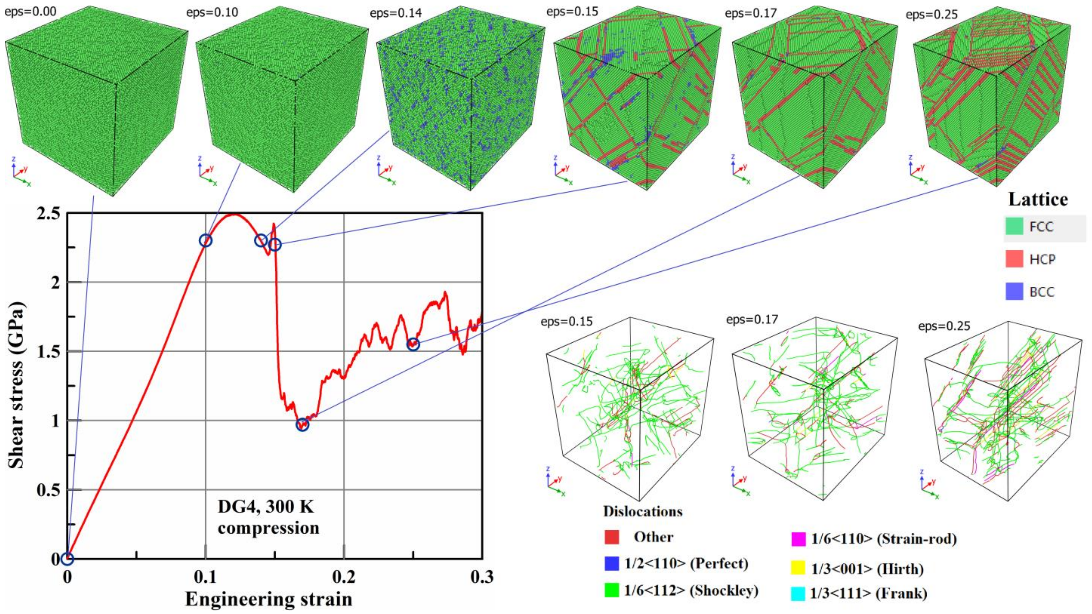
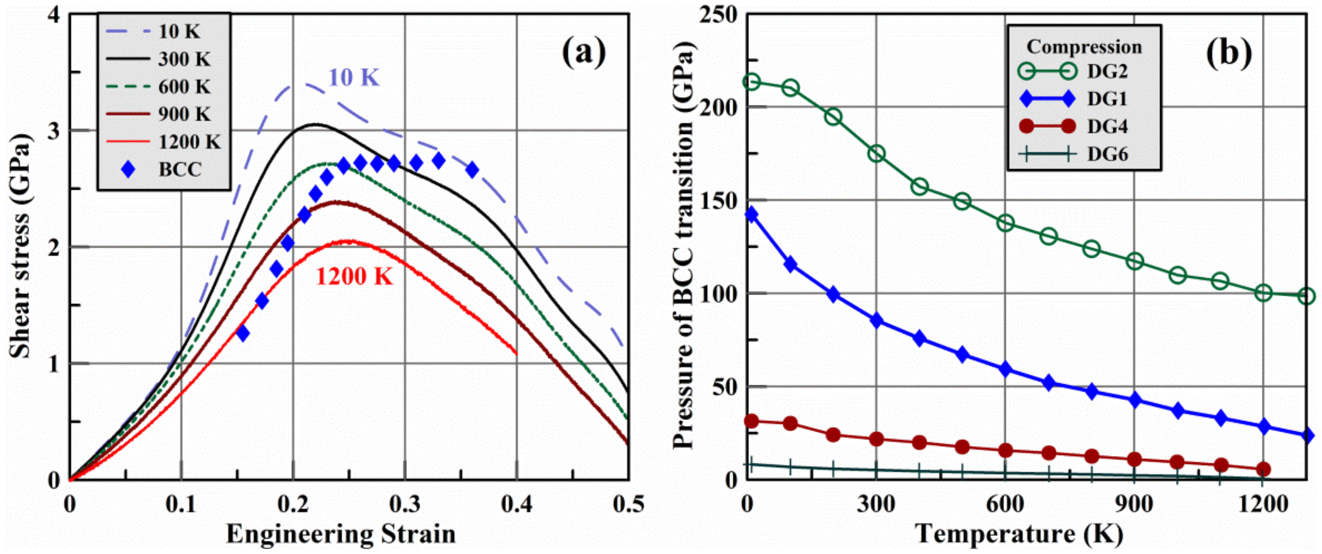
3.1. Results of MD Simulations

MD simulations of the loading of a copper single crystal along different deformation paths allowed us to investigate a wide range of axisymmetric deformed states. Figure 4 illustrates a typical evolution of MD system under compression by an example of uniaxial compression (DG4) at 300 K. The system response remains elastic until the engineering strain reaches about 0.145, after which a dislocation network forms and evolves, providing relaxation of the elastic strain. The smooth decrease in shear stress τ = σ 11 σ 22 / 2 = 3 S / 4 after the engineering strain of about 0.12 is a manifestation of non-linear elastic behavior of the material, but not a plastic relaxation. The dislocation nucleation, vice versa, leads to a short spike in the shear-stress dependence: the decrease in the elastic strain means a backward motion along the loading path and leads to an increase in shear stress before its subsequent falling down to a stress level of plastic flow. The non-zero and increasing level of plastic flow stress is explained by both the dynamic loading and strain hardening due to the high density of dislocations.
The traces of bcc phase are detected in the MD at large elastic strains (see Figure 4). For the case of compression along most deformation paths, the volume fraction of bcc phase reaches about 15–20% at the moment of dislocation nucleation and decreases after the nucleation. Thus, a partial bcc phase transition precedes the plasticity incipience in the perfect single crystal of copper. We conventionally assume an appearance of 1% of bcc phase as a beginning of this fcc–bcc phase transition. In the case of the deformation path DG1, a complete phase transition to the bcc phase is observed long before the plasticity incipience; the shear-stress curves with the marked-out points of the beginning of bcc transition are shown in Figure 5a. In the case of close-to-hydrostatic loading along the path DG0, our MD simulations reveal neither a bcc phase transition nor the dislocation nucleation. Figure 5b shows the pressure of bcc phase transition for compression along several deformation paths. One can conclude that this pressure considerably decreases with temperature and substantially varies depending on the lattice distortion, leading to the shear component of stress. The shear stress and the corresponding lattice distortion are different for different deformation paths. This conclusion is compared with the existing experimental data in the Section 4.
Figure 6 shows a typical picture of the tensile fracture of copper at negative pressure. The copper crystal remains elastic until voids and dislocations suddenly arise at a certain level of negative pressure. The beginning of plasticity is correlated with the beginning of void formation; moreover, a more intensive plasticity leading to a dense grid of staking faults is observed in the vicinity of voids at the first stage of its growth; see the atomic configuration for the engineering strain of 0.23 presented in Figure 6. On the other hand, a more detailed analysis shows that the plasticity starts somewhat earlier than the void nucleation. The time lag between these two processes depends on the deformation path. We considered initially perfect crystal without any defects. If this crystal is under hydrostatic tension, there is no average shear stress and lattice distortion, which can provoke plasticity by itself. Therefore, for close-to-hydrostatic tension, the void nucleation is the driving factor. In this case, dislocations nucleate locally in the places of future voids just before the formation of voids. An increase in the shear strains between different paths raises the influence of the average shear stress on the dislocation nucleation and on the reduction of the void nucleation threshold (see also comments in Section 3.2). Therefore, the time lag between the dislocation nucleation and void nucleation increases with the shear-strain increase, because the dislocation nucleation begins earlier and becomes the driving factor of the void formation. In all cases, this time lag for the perfect single crystal is rather small, and we neglected it in what follows.
The void nucleation and grow relax the negative pressure and even leads to a spike of positive pressure with further oscillations. This behavior of pressure at dynamic spall fracture is quite typical and is observed in MD simulations for other metals as well [64,65].
The loading paths DG6 and DG8 represent an exception: Due to a low hydrostatic component of the strain (see Figure 1b), the spall fracture is not observed in the considered range of deformation, but the dislocation nucleation takes place in both the compression part and the tension part of these deformation paths.

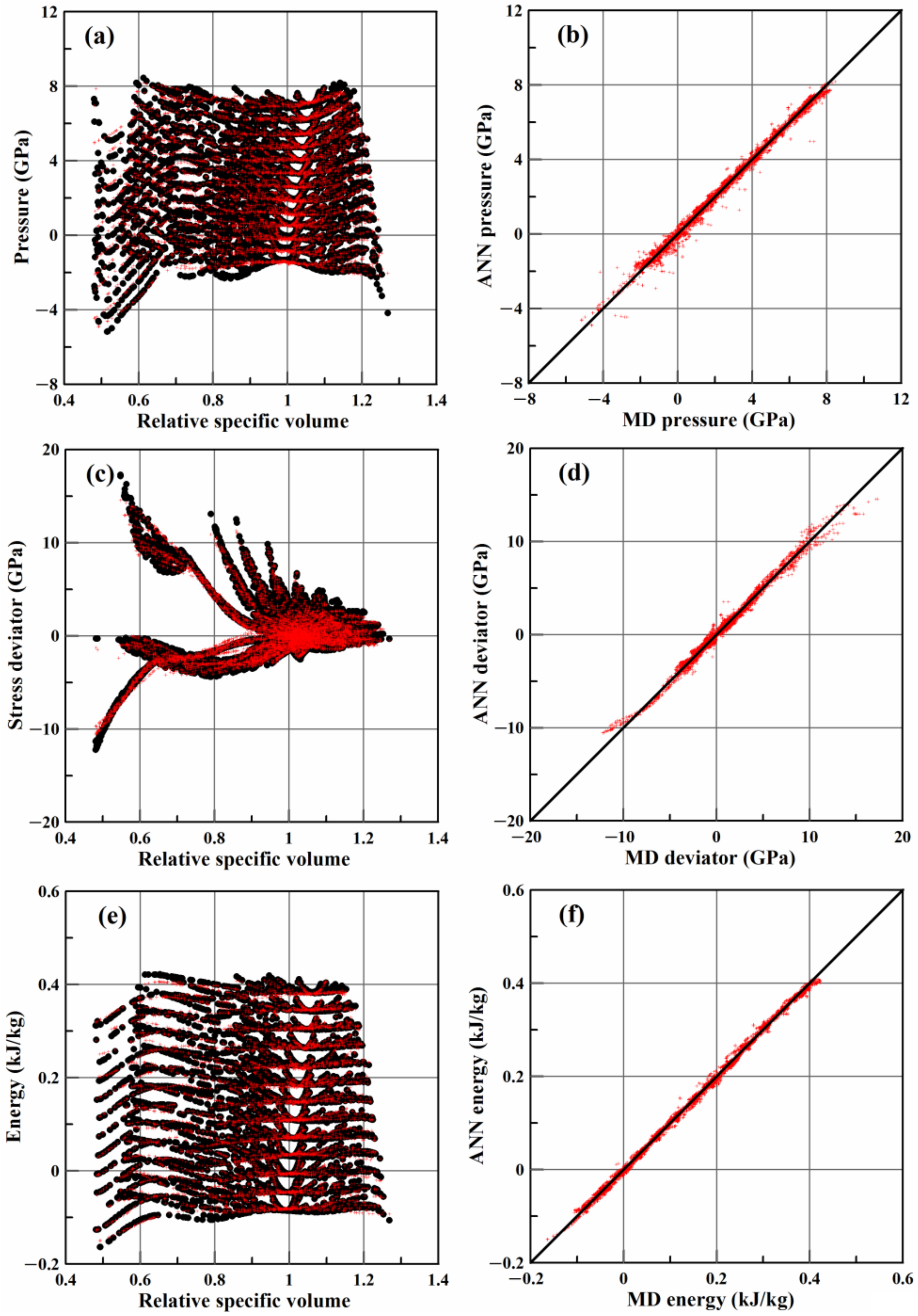
3.2. Results of ANN Training

The training results for the ANN approximating the tensor equation of state E V , E S , T P P i , S , U U i , ln K , ln G , ρ are presented in Figure 7. The ANN with four hidden layers and 64 artificial neurons in each hidden layer was used; this ANN adequately describes the complex dependencies from MD data. The four-stage training [44] allowed us to decrease the average error down to 0.8%. The obtained parameters are collected in the file “Cu.TEOS1.ANNp”, which is attached to the paper as Supplementary Materials; the structure of this file is described in Appendix A.
Figure 8 shows the dislocation nucleation threshold calculated with the strain-distance function ANN Q disl (solid lines) in comparison with the MD (circles). The threshold strains E V disl , E S disl in Figure 8a correspond to the condition Q disl E V disl , E S disl , T = 0 ; the ANN allows us to make a continuous interpolation between MD points. The stress deviator at the dislocation nucleation threshold in Figure 8b is calculated for the threshold strains E V disl , E S disl by application of the equation-of-state ANN in addition. One can see that application of these two ANNs provides an adequate correspondence of shear stress with MD points. The asymmetry with respect to the sign of the shear strain/shear stress is explained by the fact that σ 11 = P + S acts along one axial direction, while σ 22 = P S / 2 acts along two perpendicular directions. In the tensile state ( E V > 1 ) at low shear strain ( E S 0 ), the dislocation nucleation originates from the void nucleation, because formation and growth of voids involve dislocation plasticity in the vicinity of the voids. On the other hand, a hydrostatic compression ( E V < 1 and E S 0 ) does not lead to the dislocation nucleation.
The nucleation of voids takes place only for the tensile states of matter ( E V > 1 ), see Figure 9. The strain-distance function ANN Q void of the void nucleation is used in this case similar to the previously considered case of dislocation nucleation. The plotting of Figure 9b also involves the equation-of-state ANN. Figure 9b shows that increasing the absolute value of shear stress/shear strain decreases the absolute value of the threshold pressure for void nucleation. This is explained by interplay between the dislocation nucleation and void nucleation: the incipience of plasticity at additional shear deformation produces lattice defects, thus decreasing the threshold of void nucleation [66].
A similar consideration using the ANN of strain-distance function Q bcc of the bcc transformation leads to the results shown in Figure 10. This transformation goes on continuously, and the shown strain states/stress–strain states correspond to the conditional threshold of 1% transformation in the number of atoms.

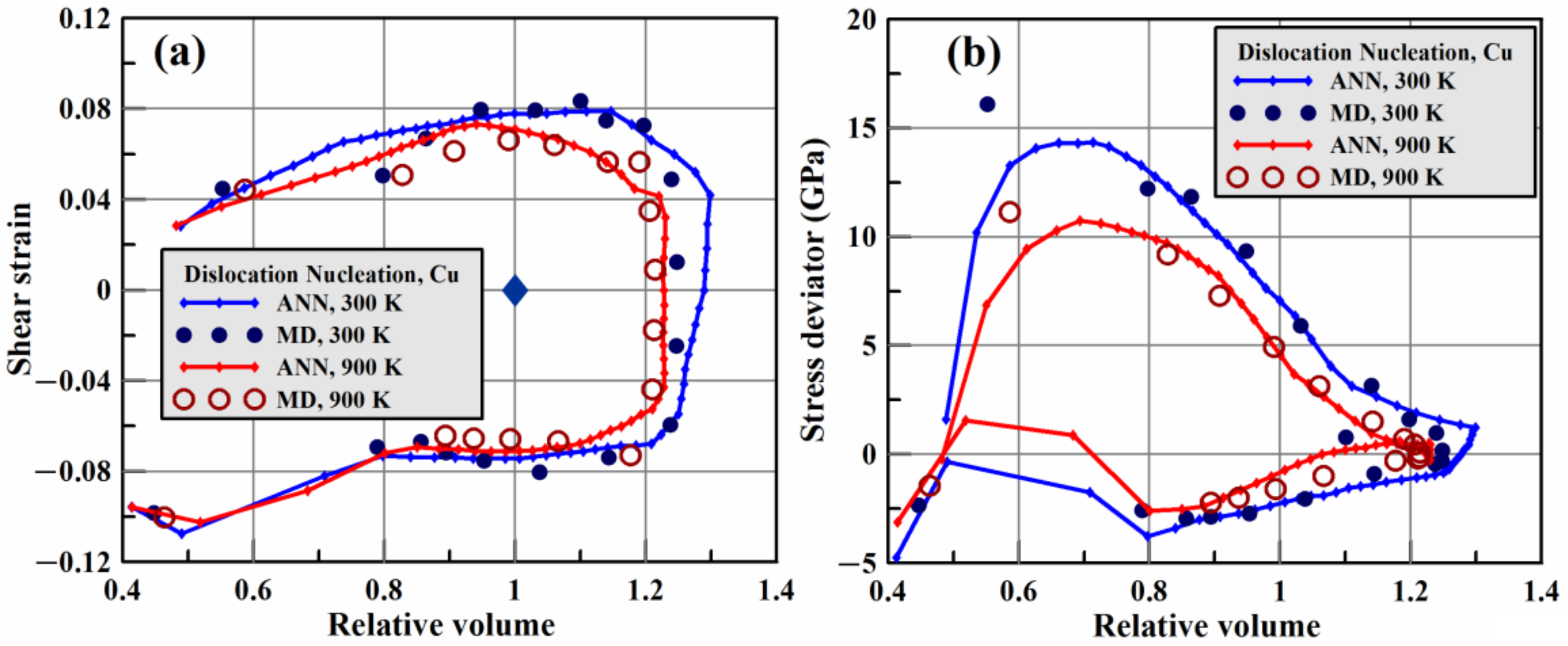
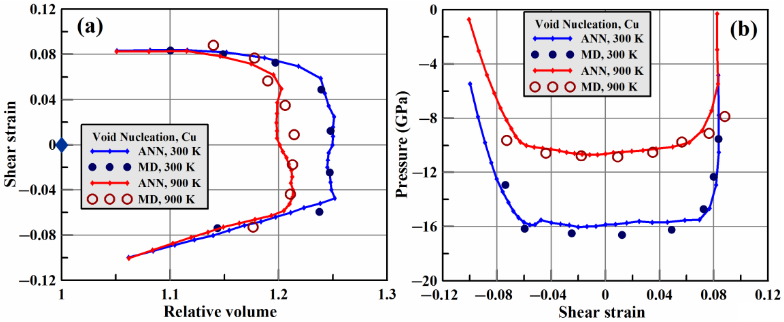
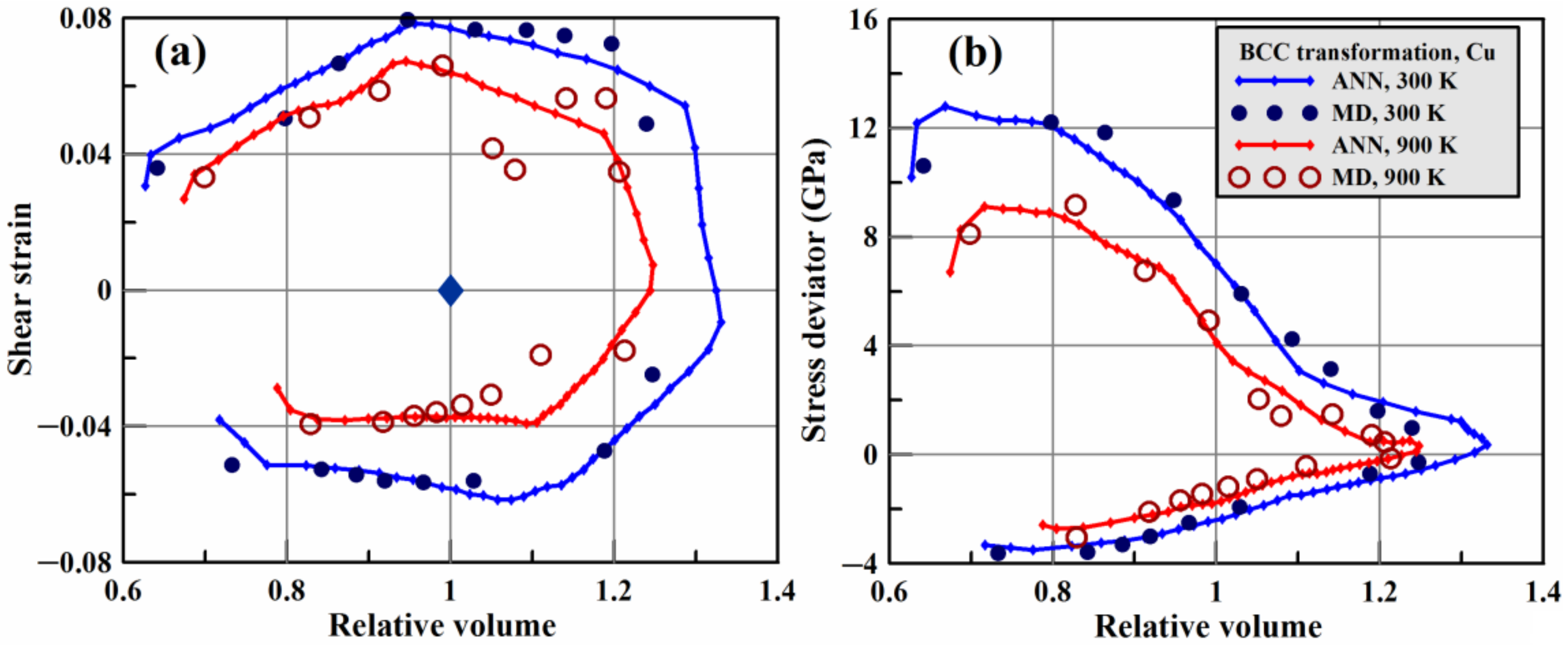
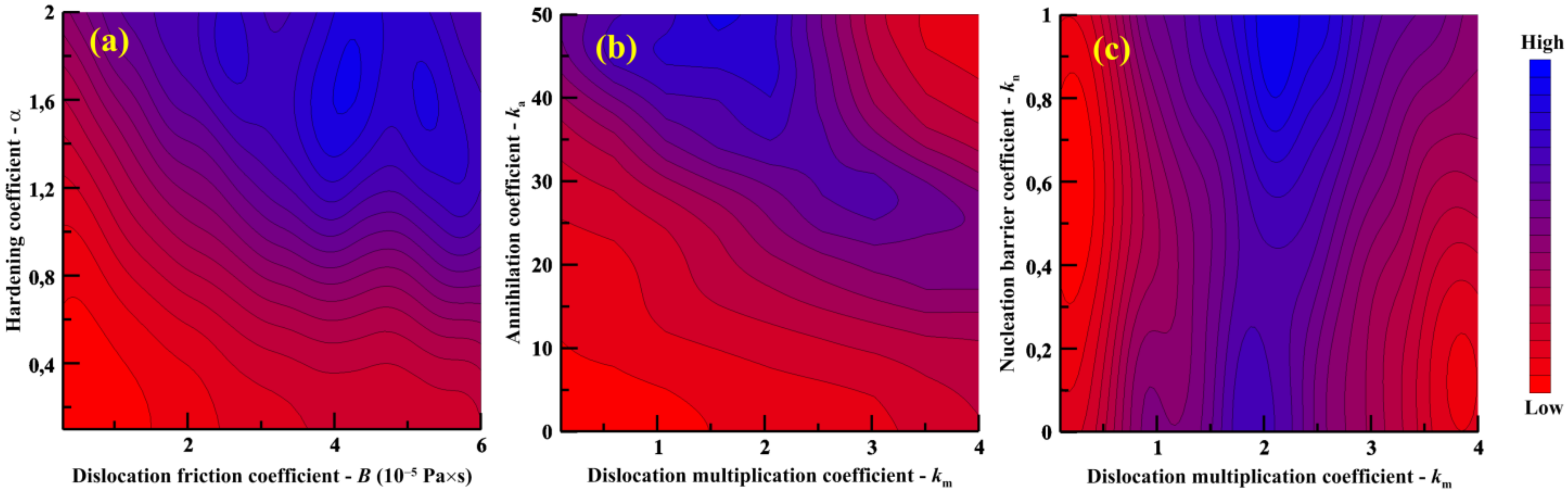
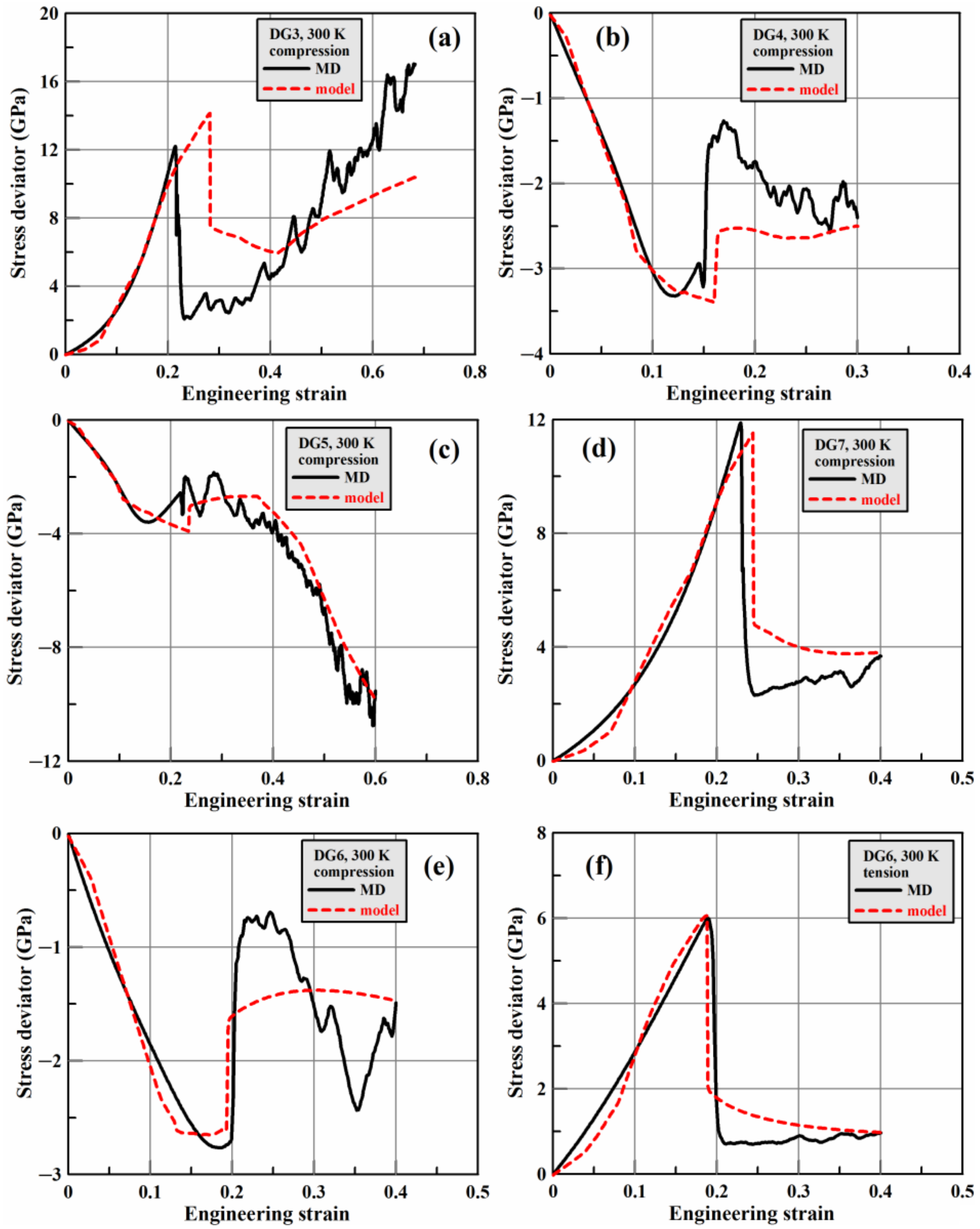
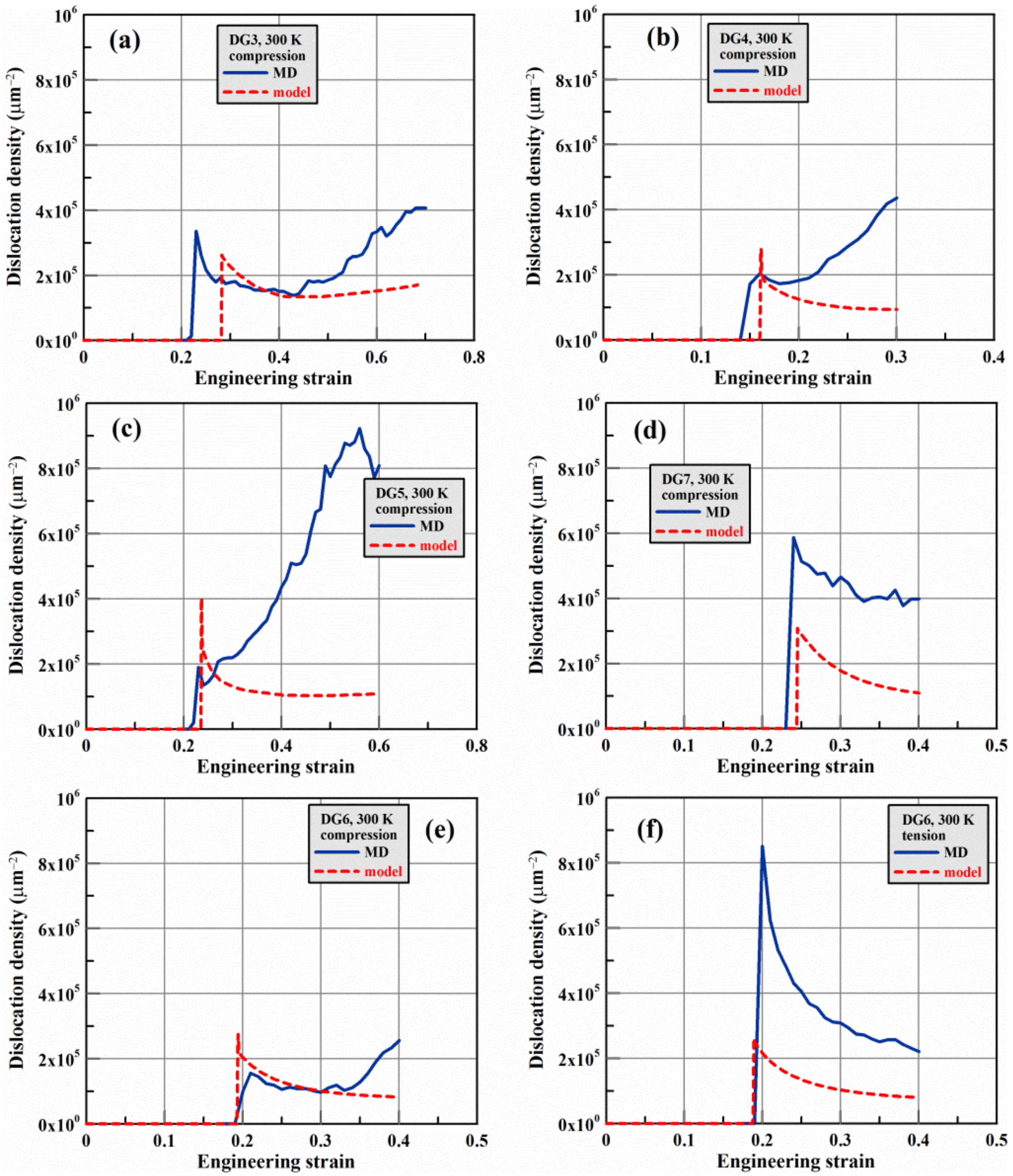
3.3. Results of Bayesian Parameterization of Dislocation Plasticity Model

For parameterization of the dislocation plasticity model, we used MD data for 300 K and for those deformation paths, leading to the nucleation of dislocations without the nucleation of voids, i.e., the compression pats of DG1, DG2, DG3, DG4 DG5, DG7 and DG9 and both compression and tension pats of DG6 and DG8. The results of Bayesian algorithm with 3500 random sets of parameters are shown in Figure 11; the considered ranges of parameters correspond to that are shown in this figure. In spite of a relatively small number of parameter sets for five adjustable parameters, the Bayesian algorithm allowed us to localize the areas of the most suitable values of these parameters.
The vertical stripe of high probability in Figure 11c shows that the used MD data are not enough to unambiguously determine the nucleation barrier coefficient, k n , while four other parameters are well-defined. The dislocation nucleation triggers the plasticity, while further kinetics is determined by the dislocation multiplication and annihilation; therefore, the system behavior is not very sensitive to the dislocation nucleation rate controlled by the coefficient k n . We chose the parameters presented in Table 2 and laying within the high probability area.
Figure 12 shows that the formulated constitutive model with these values of parameters provides an adequate description of copper deformation along various deformation paths. Calculations with other parameter sets from the high probability area show not very much difference compared with that presented in Figure 11; thus, there is no an instability of the model with respect to small variations of parameters.
Although the model parameters can depend on temperature, the calculations show that the set of parameters given in Table 2 for 300 K provides an adequate description for other temperatures as well; see Figure 13 as an example of elevated temperature. Therefore, we used this set of parameters for all considered temperatures for simplicity.
Figure 14 compares the model results for dislocation density with the MD. The dislocation density is not taken into account during the parameter identification, but the model gives adequate values for most of the deformation paths. The considerable difference in some cases is explained by simplified dislocation kinetics in the model, which takes into account only mobile Shockley dislocations, while other types of dislocations and immobilization of dislocations take place in the MD. For instance, MD data for the last frame of compression along DG4 show only about 30% fraction of the Shockley partial dislocations among other types of dislocations. Further improvement of the dislocation kinetics can solve this problem. On the other hand, the dislocation density is not a certainly defined value in the experiment, and the order-of-magnitude agreement can be considered sufficient.

4. Discussion

The homogeneous nucleation of dislocations triggers the plasticity of an initially perfect single crystal of copper at strains reaching about 0.1, and even higher, depending on the deformation path. The nonlinearity of the elastic deformation before the nucleation of dislocations manifests itself as a complex behavior of the stress deviator (Figure 3b) and dependence of pressure on the shear strain (Figure 3a). The later dependence is much weaker than the dependence of pressure on density, but it shows the effect of a partial loss of the initial crystal symmetry at large elastic shear deformations. The room-temperature isotherm from our MD simulations with EAM potential [40] coincides with the experimental data [50] and DFT calculations [51] (see Figure 2a). This coincidence verifies the used interatomic potential.
Compression along the trajectories close to the hydrostatic compression (DG0, DG1 and DG2) leads to a rapid increase in pressure at a slow increase in shear stress. As a result, the homogeneous nucleation of dislocations is either delayed (for DG1 and DG2) or completely suppressed (for DG0); see Figure 8a. Under tension, the dislocation nucleation and void nucleation are interconnected. The nucleating voids induce plastic flow and dislocations in their vicinity; this is the dominant process of dislocation nucleation at low shear stress. In this case, the nucleation of both types of lattice defects, voids and dislocations occurs almost simultaneously at a certain level of negative pressure; see Figure 9b. On the other hand, an increase in the shear stress provokes the dislocation nucleation as the leading process, while voids nucleate on the formed lattice defects at less negative pressure; see Figure 9b. In this case, the dislocations can nucleate substantially earlier than voids; in the particular case of tension along DG6 and DG8, we observe the dislocation nucleation, but we do not observe the void nucleation for the considered tensile strains.
Figure 9b shows that the level of negative pressure required for the void nucleation as a starting point of spall fracture decreases from about 16 GPa for 300 K to about 10 GPa for 900 K at low shear component of strain in both cases. These values of the spall strength of copper coincide with the experimental results [67,68], giving the range of 11–18 GPa for the close strain rates of (0.1–0.3) × 109 s−1. This coincidence additionally verifies the used interatomic potential [40].
Our MD simulations do not indicate an fcc–bcc phase transition in copper up to a pressure of 500 GPa in the case of the deformation path DG0, which is close to a hydrostatic compression. For other compression paths, a partial or complete (DG1) bcc transition takes place, and the pressure of this phase transition decreases with the increase in the shear component of strain and with the temperature rise. The shear component of strain reflects the elastic part of deformation and the corresponding distortion of the crystal lattice. At room temperature, the pressure of the bcc phase transition reaches about 170 GPa for the deformation path DG2, but it consists of only about 20 GPa for the uniaxial compression along the deformation path DG4 (see Figure 5). It should be mentioned that our MD data were obtained for an initially perfect single crystal of copper, which did not contain dislocations and traces of plasticity before the phase transition. Therefore, the response was elastic, and the shear component of strain was completely determined by the deformation path.
Our results on bcc transformation shed light on the existing experimental data for the shock-wave compression [69], ramp compression [70] and quasi-static loading in diamond anvil cell [50], which seem somewhat contradictory. The quasi-static measurements [50] show the stability of the ambient fcc phase of copper up to 150 GPa in the absence of non-hydrostatic stresses. According to Reference [70], copper retains its ambient fcc structure under dynamic ramp compression to 1150 GPa, while according to Reference [69], a shock compression to about 180 GPa initiates transformation into the bcc structure. All of these experiments were performed for polycrystals with initial defects tending to relax the shear stress and elastic shear strain, i.e., to decrease the distortion of the crystal lattice. This relaxation is most pronounced for the quasi-static compression in the diamond anvil cell and for the dynamic ramp compression with relatively low stain rate: The absence of the elastic shear strain and corresponding distortion suppresses the transformation to the bcc structure and makes the ambient fcc phase stable even under such strong pressure. The shock compression with higher strain rate retains a substantial shear stress due to the finite rate of plastic relaxation, and this shear stress/elastic shear strain makes possible the phase transition to bcc. Another factor that is favorable for the phase transformation is the increase in temperature in the case of shock loading. Due to the plastic relaxation in the course of shock compression, the shear strain in this case is weaker than for the uniaxial compression (DG4) of the perfect single crystal studied in our MD simulations. Therefore, as reported in Reference [69], pressure of bcc transformation (180 GPa) is much higher than that for DG4 (20 GPa, even at the room temperature). In our opinion, the correlation discovered in Reference [69] between the bcc transformation and the arising of stacking faults is explained by the existence and fast relaxation of shear stress under the shock loading. In our MD results, partial bcc transition precedes the dislocation activity, resulting in the multiple stacking faults left behind by Shockley partial dislocations. The calculated fraction of the hcp phase (stacking faults) is above 10%, which correlates with the X-ray measurements [69].
We developed a new approach for construction of MD-informed constitutive model of material with machine learning. This approach combines ANN approximation of unambiguous state functions, such as the equation of state and the threshold of dislocation nucleation, with the kinetics model for description of the plastic flow after the dislocation nucleation. By an example of copper single crystal, we show the efficiency of the developed approach in the description of the elastic–plastic deformation along various loading paths (Figure 12 and Figure 13). At the elastic stage before the dislocation nucleation, the correspondence depends on the precision of the trained ANNs for the tensor equation of state and nucleation threshold. In the training dataset for the equation of state ANN, we disregard the data with negative value of the local shear modulus, G , defined by Equation (6), because we need to calculate the transverse sound speed, c t = G / ρ (see Equation (20)), and we use ln G in the equation of state ANN to ensure the positivity of the shear modulus. Therefore, we see an extrapolation by the ANN for the parts of the stress deviator–strain curve after the shear stress minimum/maximum and before the dislocation nucleation in Figure 12b,c and Figure 13b,c. Expansion of the training dataset on and behind the border of the elastic range can increases the precision in this part. This expansion requires a more accurate determination of the transverse sound speed as the value connected with the shear modulus relative to the shear in the direction of the Burgers vector of the Shockley partial dislocation rather than the axial strain used in Equation (6). After the plasticity incipience, the precision can be increased by using a more complex dislocation plasticity model, for instance, with the accounting of immobilized dislocations. In spite of this comment, the present model provides a quite adequate description of the MD data. Another possible direction of the development of the present approach is the incorporation of the kinetics models for spall fracture and bcc phase transition.

5. Conclusions

We developed a new approach for constructing a constitutive model that describes both high strain rates and severe strains. Molecular dynamics data were incorporated into the constitutive model by means of machine learning. Artificial neural networks were used to approximate unambiguous state functions, such as the elastic stress–strain relation (tensor equation of state), the dislocation nucleation threshold, the void nucleation threshold and the beginning of bcc transformation. On the other hand, the kinetic process of plasticity was described by the time-differential equations of the dislocation plasticity model; the molecular dynamics data were used to fit model parameters by means of a probabilistic Bayesian algorithm. We applied and verified this approach in the case of axisymmetric deformation of copper single crystal; the problem statement relates to loading by plane shock waves and related issues. The equation system of elastic–plastic deformation under the shock-wave loading was formulated, but a detailed investigation of the structure and evolution of shock waves on the basis of this model remains for future work.

Supplementary Materials

The following are available online at https://www.mdpi.com/article/10.3390/met12030402/s1. File “Files.ANNp.xlsx”, with the following worksheets: “Cu.TEOS1.ANNp”, with parameters of ANN for tensor equation of state for copper under axisymmetric deformation; “Cu.DISL1.ANNp”, with parameters of ANN for the strain-distance function of dislocation nucleation, Q disl ; “Cu.VOID1.ANNp”, with parameters of ANN for the strain-distance function of void nucleation Q void ; and “Cu.BCC1.ANNp”, with parameters of ANN for the strain-distance function of bcc transformation, Q bcc .

Author Contributions

Conceptualization, A.E.M.; methodology, A.E.M., M.V.L., N.A.G. and E.V.F.; software, A.E.M.; validation, A.E.M. and M.V.L.; formal analysis, A.E.M., M.V.L., N.A.G. and E.V.F.; investigation, A.E.M., M.V.L. and N.A.G.; resources, A.E.M.; data curation, A.E.M.; writing—original draft preparation, A.E.M.; writing—review and editing, A.E.M.; visualization, A.E.M.; supervision, A.E.M.; project administration, A.E.M.; funding acquisition, A.E.M. All authors have read and agreed to the published version of the manuscript.

Funding

This research and the APC were funded by the RUSSIAN SCIENCE FOUNDATION, grant number 20-11-20153.

Institutional Review Board Statement

Not applicable.

Informed Consent Statement

Not applicable.

Data Availability Statement

The developed tensor equation of state of copper and the strain-distance functions for dislocation nucleation, void nucleation and bcc transformation in the form of parameter files of the trained ANNs are available as Supplementary Materials; the structure of this file is described in the Appendix A. Other data are available upon request.

Conflicts of Interest

The authors declare no conflict of interest.

Appendix A

The parameters of the trained ANNs are attached as Supplementary Materials to this paper. The description of ANN parameter files is given in Table A1. The structure of the ANN corresponds to that is proposed in Reference [44]. The first line contains the number of layers, L , of artificial neurons. The second line contains the numbers of neurons in each layer printed sequentially: N 1 , N 2 , N 3 , , N L . The type of transfer function is not explicitly specified in the files, but “Leaky ReLU” transfer function is used for hidden layers, and “Sigmoid” transfer function is used for the output layer. The third line should be missed. The weights a j k , m are printed starting, from the fourth line, in the following order: a 21 , 1 , a 21 , 2 , …, a 21 , N 1 ; line feed; a 22 , 1 , a 22 , 2 , …, a 22 , N 1 ; line feed; …, a 2 N 2 , N 1 ; empty line; a 31 , 1 , a 31 , 2 , a 31 , 2 , …, a 31 , N 2 ; line feed; a 32 , 1 , a 32 , 2 , …, a 32 , N 2 ; line feed; …, a 3 N 3 , N 2 ; empty line, etcetera. The next line after the ending of the weight’s section should be missed. Following this, the biases b j k are printed in the same order: b 21 , b 22 , …, b 2 N 2 ; empty line; b 31 , b 32 , …, b 3 N 3 ; empty line, etcetera. The next line after the ending of the biases section should be missed. The following N 1 + N L lines contain minimal and maximal values for ANN inputs and outputs. All the input values, X ˜ i , before being used in ANN, should be normalized as X i = X ˜ i X i min / X i max X i min . On the other hand, all the outputs, Y i , should be restored as Y ˜ i = Y i min + Y i Y i max Y i min .
Table A1. Description of ANN parameter files.
ParameterCu.TEOS1.ANNpCu.DISL1.ANNpCu.VOID1.ANNpCu.BCC1.ANNp
Number of inputs3
Inputs E V , E S , T
Number of outputs6111
Outputs P P i , S , U U i , ln K , ln G , ρ Q disl Q void Q bcc

References

  1. Gurrutxaga-Lerma, B.; Shehadeh, M.A.; Balint, D.S.; Dini, D.; Chen, L.; Eakins, D.E. The effect of temperature on the elastic precursor decay in shock loaded FCC aluminium and BCC iron. Int. J. Plast. 2017, 96, 135–155. [Google Scholar] [CrossRef]
  2. Kanel, G.I.; Savinykh, A.S.; Garkushin, G.V.; Razorenov, S.V. Effects of temperature on the flow stress of aluminum in shock waves and rarefaction waves. J. Appl. Phys. 2020, 127, 035901. [Google Scholar] [CrossRef]
  3. Kanel, G.I.; Savinykh, A.S.; Garkushin, G.V.; Razorenov, S.V. Effects of temperature and strain on the resistance to high-rate deformation of copper in shock waves. J. Appl. Phys. 2020, 128, 115901. [Google Scholar] [CrossRef]
  4. Savinykh, A.S.; Kanel, G.I.; Garkushin, G.V.; Razorenov, S.V. Resistance to high-rate deformation and fracture of lead at normal and elevated temperatures in the sub-microsecond time range. J. Appl. Phys. 2020, 128, 025902. [Google Scholar] [CrossRef]
  5. Kanel, G.I.; Savinykh, A.S.; Garkushin, G.V.; Razorenov, S.V. High-rate deformation of titanium in shock waves at normal and elevated temperatures. J. Exp. Theor. Phys. 2021, 132, 438–445. [Google Scholar] [CrossRef]
  6. Saveleva, N.V.; Bayandin, Y.V.; Savinykh, A.S.; Garkushin, G.V.; Razorenov, S.V.; Naimark, O.B. The formation of elastoplastic fronts and spall fracture in AMg6 alloy under shock-wave loading. Tech. Phys. Lett. 2018, 44, 823–826. [Google Scholar] [CrossRef]
  7. Brodova, I.G.; Petrova, A.N.; Shirinkina, I.G.; Rasposienko, D.Y.; Yolshina, L.A.; Muradymov, R.V.; Razorenov, S.V.; Shorokhov, E.V. Mechanical properties of submicrocrystalline aluminium matrix composites reinforced by “in situ” graphene through severe plastic deformation processes. J. Alloy. Compd. 2021, 859, 158387. [Google Scholar] [CrossRef]
  8. Ivanov, K.V.; Razorenov, S.V.; Garkushin, G.V. Investigation of structure and mechanical properties under quasi-static and planar impact loading of aluminum composite reinforced with Al2O3 nanoparticles of different shape. Mater. Today Commun. 2021, 29, 102942. [Google Scholar] [CrossRef]
  9. Klimova-Korsmik, O.; Turichin, G.; Mendagaliyev, R.; Razorenov, S.; Garkushin, G.; Savinykh, A.; Korsmik, R. High-strain deformation and spallation strength of 09CrNi2MoCu steel obtained by direct laser deposition. Metals 2021, 11, 1305. [Google Scholar] [CrossRef]
  10. Promakhov, V.; Schulz, N.; Vorozhtsov, A.; Savinykh, A.; Garkushin, G.; Razorenov, S.; Klimova-Korsmik, O. The strength of inconel 625, manufactured by the method of direct laser deposition under sub-microsecond load duration. Metals 2021, 11, 1796. [Google Scholar] [CrossRef]
  11. Khishchenko, K.V.; Mayer, A.E. High- and low-entropy layers in solids behind shock and ramp compression waves. Int. J. Mech. Sci. 2021, 189, 105971. [Google Scholar] [CrossRef]
  12. Moshe, E.; Eliezer, S.; Dekel, E.; Ludmirsky, A.; Henis, Z.; Werdiger, M.; Goldberg, I.B.; Eliaz, N.; Elieser, D. An increase of the spall strength in aluminum, copper, and Metglas at strain rates larger than 107 s−1. J. Appl. Phys. 1998, 83, 4004. [Google Scholar] [CrossRef] [Green Version]
  13. Krasyuk, I.K.; Pashinin, P.P.; Semenov, A.Y.; Khishchenko, K.V.; Fortov, V.E. Study of extreme states of matter at high energy densities and high strain rates with powerful lasers. Laser Phys. 2016, 26, 094001. [Google Scholar] [CrossRef] [Green Version]
  14. Ashitkov, S.I.; Komarov, P.S.; Struleva, E.V.; Agranat, M.B.; Kanel, G.I. Mechanical and optical properties of vanadium under shock picosecond loads. JETP Lett. 2015, 101, 276–281. [Google Scholar] [CrossRef]
  15. Kanel, G.I.; Zaretsky, E.B.; Razorenov, S.V.; Ashitkov, S.I.; Fortov, V.E. Unusual plasticity and strength of metals at ultra-short load durations. Phys. Uspekhi 2017, 60, 490–508. [Google Scholar] [CrossRef] [Green Version]
  16. Zuanetti, B.; McGrane, S.D.; Bolme, C.A.; Prakash, V. Measurement of elastic precursor decay in pre-heated aluminum films under ultra-fast laser generated shocks. J. Appl. Phys. 2018, 123, 195104. [Google Scholar] [CrossRef] [Green Version]
  17. Murzov, S.; Ashitkov, S.; Struleva, E.; Komarov, P.; Zhakhovsky, V.; Khokhlov, V.; Inogamov, N. Elastoplastic and polymorphic transformations of iron at ultra-high strain rates in laser-driven shock waves. J. Appl. Phys. 2021, 130, 245902. [Google Scholar] [CrossRef]
  18. Shao, J.-L.; Guo, X.-X.; Lu, G.; He, W.; Xin, J. Influence of shear wave on the HCP nucleation in BCC iron under oblique shock conditions. Mech. Mater. 2021, 158, 103878. [Google Scholar] [CrossRef]
  19. Jiang, D.-D.; Shao, J.-L.; Wu, B.; Wang, P.; He, A.-M. Sudden change of spall strength induced by shock defects based on atomistic simulation of single crystal aluminum. Scr. Mater. 2022, 210, 114474. [Google Scholar] [CrossRef]
  20. Wang, J.-N.; Wu, B.; Wu, F.-C.; Wang, P.; He, A.-M.; Wu, H.-A. Spall and recompression processes with double shock loading of polycrystalline copper. Mech. Mater. 2022, 165, 104194. [Google Scholar] [CrossRef]
  21. Austin, R.A.; McDowell, D.L. A dislocation-based constitutive model for viscoplastic deformation of fcc metals at very high strain rates. Int. J. Plast. 2011, 27, 1–24. [Google Scholar] [CrossRef]
  22. Krasnikov, V.S.; Mayer, A.E.; Yalovets, A.P. Dislocation based high-rate plasticity model and its application to plate-impact and ultra short electron irradiation simulations. Int. J. Plast. 2011, 27, 1294–1308. [Google Scholar] [CrossRef]
  23. Lloyd, J.T.; Clayton, J.D.; Austin, R.A.; McDowell, D.L. Plane wave simulation of elastic-viscoplastic single crystals. J. Mech. Phys. Solids 2014, 69, 14–32. [Google Scholar] [CrossRef]
  24. Zuanetti, B.; Luscher, D.J.; Ramos, K.; Bolme, C. Unraveling the implications of finite specimen size on the interpretation of dynamic experiments for polycrystalline aluminum through direct numerical simulations. Int. J. Plast. 2021, 145, 103080. [Google Scholar] [CrossRef]
  25. Gurrutxaga–Lerma, B.; Verschueren, J.; Sutton, A.P.; Dini, D. The mechanics and physics of high-speed dislocations: A critical review. Int. Mater. Rev. 2021, 66, 215–255. [Google Scholar] [CrossRef]
  26. Shen, Y.; Spearot, D.E. Mobility of dislocations in FeNiCrCoCu high entropy alloys. Modell. Simul. Mater. Sci. Eng. 2021, 29, 085017. [Google Scholar] [CrossRef]
  27. Bryukhanov, I.A.; Emelyanov, V.A. Shear stress relaxation through the motion of edge dislocations in Cu and Cu–Ni solid solution: A molecular dynamics and discrete dislocation study. Comput. Mater. Sci. 2022, 201, 110885. [Google Scholar] [CrossRef]
  28. Esteban-Manzanares, G.; Bellón, B.; Martínez, E.; Papadimitriou, I.; LLorca, J. Strengthening of Al–Cu alloys by Guinier–Preston zones: Predictions from atomistic simulations. J. Mech. Phys. Solids 2019, 132, 103675. [Google Scholar] [CrossRef] [Green Version]
  29. Rajput, A.; Paul, S.K. Effect of soft and hard inclusions in tensile deformation and damage mechanism of Aluminum: A molecular dynamics study. J. Alloy. Compd. 2021, 869, 159213. [Google Scholar] [CrossRef]
  30. Krasnikov, V.S.; Mayer, A.E.; Pogorelko, V.V.; Gazizov, M.R. Influence of θ’ phase cutting on precipitate hardening of Al–Cu alloy during prolonged plastic deformation: Molecular dynamics and continuum modeling. Appl. Sci. 2021, 11, 4906. [Google Scholar] [CrossRef]
  31. Shang, H.; Wu, P.; Lou, Y.; Wang, J.; Chen, Q. Machine learning-based modeling of the coupling effect of strain rate and temperature on strain hardening for 5182-O aluminum alloy. J. Mater. Process. Technol. 2022, 302, 117501. [Google Scholar] [CrossRef]
  32. Li, X.; Roth, C.C.; Bonatti, C.; Mohr, D. Counterexample-trained neural network model of rate and temperature dependent hardening with dynamic strain aging. Int. J. Plast. 2022, 151, 103218. [Google Scholar] [CrossRef]
  33. Bonatti, C.; Mohr, D. On the importance of self-consistency in recurrent neural network models representing elasto-plastic solids. J. Mech. Phys. Solids. 2022, 158, 104697. [Google Scholar] [CrossRef]
  34. Gracheva, N.A.; Lekanov, M.V.; Mayer, A.E.; Fomin, E.V. Application of neural networks for modeling shock-wave processes in aluminum. Mech. Solids 2021, 56, 326–342. [Google Scholar] [CrossRef]
  35. Mayer, A.E.; Krasnikov, V.S.; Pogorelko, V.V. Homogeneous nucleation of dislocations in copper: Theory and approximate description based on molecular dynamics and artificial neural networks. Comput. Mater. Sci. 2022, 206, 111266. [Google Scholar] [CrossRef]
  36. Ma, K.; Chen, J.; Dongare, A.M. Role of pre-existing dislocations on the shock compression and spall behavior in single-crystal copper at atomic scales. J. Appl. Phys. 2021, 129, 175901. [Google Scholar] [CrossRef]
  37. Wang, S.; Pan, H.; Wang, X.; Yin, J.; Hu, X.; Xu, W.; Wang, P. Atomic insights into the quasi-elastic response in shock reloading of shocked metals. Results Phys. 2021, 31, 104954. [Google Scholar] [CrossRef]
  38. Bryukhanov, I.A. Atomistic simulation of the shock wave in copper single crystals with pre-existing dislocation network. Int. J. Plast. 2022, 151, 103171. [Google Scholar] [CrossRef]
  39. Plimpton, S.J. Fast parallel algorithms for short-range molecular dynamics. J. Comp. Phys. 1995, 117, 1–19. [Google Scholar] [CrossRef] [Green Version]
  40. Mishin, Y.; Mehl, M.J.; Papaconstantopoulos, D.A.; Voter, A.F.; Kress, J.D. Structural stability and lattice defects in copper: Ab initio, tight-binding, and embedded-atom calculations. Phys. Rev. B 2001, 63, 224106. [Google Scholar] [CrossRef] [Green Version]
  41. Mase, G.E. Theory and Problems of Continuum Mechanics; McGraw-Hill: New York, NY, USA, 1970. [Google Scholar]
  42. Hoover, W.G. Canonical dynamics: Equilibrium phase-space distributions. Phys. Rev. A 1985, 31, 1695–1697. [Google Scholar] [CrossRef] [PubMed] [Green Version]
  43. Ogata, S.; Li, J.; Yip, S. Ideal pure shear strength of aluminum and copper. Science 2002, 298, 807–811. [Google Scholar] [CrossRef] [Green Version]
  44. Mayer, A.E.; Krasnikov, V.S.; Pogorelko, V.V. Dislocation nucleation in Al single crystal at shear parallel to (111) plane: Molecular dynamics simulations and nucleation theory with artificial neural networks. Int. J. Plast. 2021, 139, 102953. [Google Scholar] [CrossRef]
  45. Larsen, P.M.; Schmidt, S.; SchiØtz, J. Robust structural identification via polyhedral template matching. Model. Simul. Mater. Sci. Eng. 2016, 24, 055007. [Google Scholar] [CrossRef]
  46. Stukowski, A.; Bulatov, V.V.; Arsenlis, A. Automated identification and indexing of dislocations in crystal interfaces. Model. Simul. Mater. Sci. Eng. 2012, 20, 085007. [Google Scholar] [CrossRef]
  47. Stukowski, A. Computational analysis methods in atomistic modeling of crystals. JOM 2014, 66, 399–407. [Google Scholar] [CrossRef]
  48. Stukowski, A. Visualization and analysis of atomistic simulation data with OVITO—The Open Visualization Tool. Model. Simul. Mater. Sci. Eng. 2010, 18, 015012. [Google Scholar] [CrossRef]
  49. Thompson, A.P.; Plimpton, S.J.; Mattson, W. General formulation of pressure and stress tensor for arbitrary many-body interaction potentials under periodic boundary conditions. J. Chem. Phys. 2009, 131, 154107. [Google Scholar] [CrossRef] [Green Version]
  50. Dewaele, A.; Loubeyre, P.; Mezouar, M. Equations of state of six metals above 94 GPa. Phys. Rev. B 2004, 70, 094112. [Google Scholar] [CrossRef] [Green Version]
  51. Greeff, C.W.; Boettger, J.C.; Graf, M.J.; Johnson, J.D. Theoretical investigation of the Cu EOS standard. J. Phys. Chem. Solids 2006, 67, 2033–2040. [Google Scholar] [CrossRef]
  52. Popova, T.V.; Mayer, A.E.; Khishchenko, K.V. Evolution of shock compression pulses in polymethylmethacrylate and aluminum. J. Appl. Phys. 2018, 123, 235902. [Google Scholar] [CrossRef]
  53. Khan, A.S.; Liu, J.; Yoon, J.W.; Nambori, R. Strain rate effect of high purity aluminum single crystals: Experiments and simulations. Int. J. Plast. 2015, 67, 39–52. [Google Scholar] [CrossRef]
  54. Nguyen, T.; Luscher, D.J.; Wilkerson, J.W. A dislocation-based crystal plasticity framework for dynamic ductile failure of single crystals. J. Mech. Phys. Solids 2017, 108, 1–29. [Google Scholar] [CrossRef]
  55. Khan, A.S.; Liu, J. A deformation mechanism based crystal plasticity model of ultrafine-grained/nanocrystalline FCC polycrystals. Int. J. Plast. 2016, 86, 56–69. [Google Scholar] [CrossRef]
  56. Selyutina, N.; Borodin, E.N.; Petrov, Y.; Mayer, A.E. The definition of characteristic times of plastic relaxation by dislocation slip and grain boundary sliding in copper and nickel. Int. J. Plast. 2016, 82, 97–111. [Google Scholar] [CrossRef]
  57. Hirth, J.P.; Lothe, J. Theory of Dislocations; Wiley & Sons: New York, NY, USA, 1982. [Google Scholar]
  58. Nguyen, T.; Fensin, S.J.; Luscher, D.J. Dynamic crystal plasticity modeling of single crystal tantalum and validation using Taylor cylinder impact tests. Int. J. Plast. 2021, 139, 102940. [Google Scholar] [CrossRef]
  59. Mayer, A.E. Micromechanical model of nanoparticle compaction and shock waves in metal powders. Int. J. Plast. 2021, 147, 103102. [Google Scholar] [CrossRef]
  60. Kuropatenko, V.F. New models of continuum mechanics. J. Eng. Phys. 2011, 84, 77–99. [Google Scholar] [CrossRef]
  61. VonNeumann, J.; Richtmyer, R.D. A Method for the numerical calculation of hydrodynamic shocks. J. Appl. Phys. 1950, 21, 232–237. [Google Scholar] [CrossRef]
  62. Kuropatenko, V.F. On a difference method for the calculation of shock waves. USSR Comput. Math. Math. Phys. 1963, 3, 268–273. [Google Scholar] [CrossRef]
  63. Yalovets, A.P. Calculation of flows of a medium induced by high-power beams of charged particles. J. Appl. Mech. Tech. Phys. 1997, 38, 137–150. [Google Scholar] [CrossRef]
  64. Mayer, A.E.; Mayer, P.N. Evolution of pore ensemble in solid and molten aluminum under dynamic tensile fracture: Molecular dynamics simulations and mechanical models. Int. J. Mech. Sci. 2019, 157–158, 816–832. [Google Scholar] [CrossRef]
  65. Mayer, A.E.; Mayer, P.N. Strain rate dependence of spall strength for solid and molten lead and tin. Int. J. Fract. 2020, 222, 171–195. [Google Scholar] [CrossRef]
  66. Krasnikov, V.S.; Mayer, A.E. Initial stage of fracture of aluminum with ideal and defect lattice. J. Phys. Conf. Ser. 2015, 653, 012094. [Google Scholar] [CrossRef]
  67. Moshe, E.; Eliezer, S.; Henis, Z.; Werdiger, M.; Dekel, E.; Horovitz, Y.; Maman, S.; Goldberg, I.B.; Eliezer, D. Experimental measurements of the strength of metals approaching the theoretical limit predicted by the equation of state. Appl. Phys. Let. 2000, 76, 1555. [Google Scholar] [CrossRef]
  68. Werdiger, M.; Eliezer, S.; Moshe, E.; Henis, Z.; Dekel, E.; Horovitz, Y.; Arad, B. Al and Cu dynamic strength at a strain rate of 5*108 s–1. AIP Conf. Proc. 2002, 620, 583. [Google Scholar] [CrossRef]
  69. Sharma, S.M.; Turneaure, S.J.; Winey, J.M.; Gupta, Y.M. Transformation of shock-compressed copper to the body-centered-cubic structure at 180 GPa. Phys. Rev. B 2020, 102, 020103. [Google Scholar] [CrossRef]
  70. Fratanduono, D.E.; Smith, R.F.; Ali, S.J.; Braun, D.G.; Fernandez-Pañella, A.; Zhang, S.; Kraus, R.G.; Coppari, F.; McNaney, J.M.; Marshall, M.C.; et al. Probing the solid phase of noble metal copper at terapascal conditions. Phys. Rev. Lett. 2020, 124, 015701. [Google Scholar] [CrossRef]
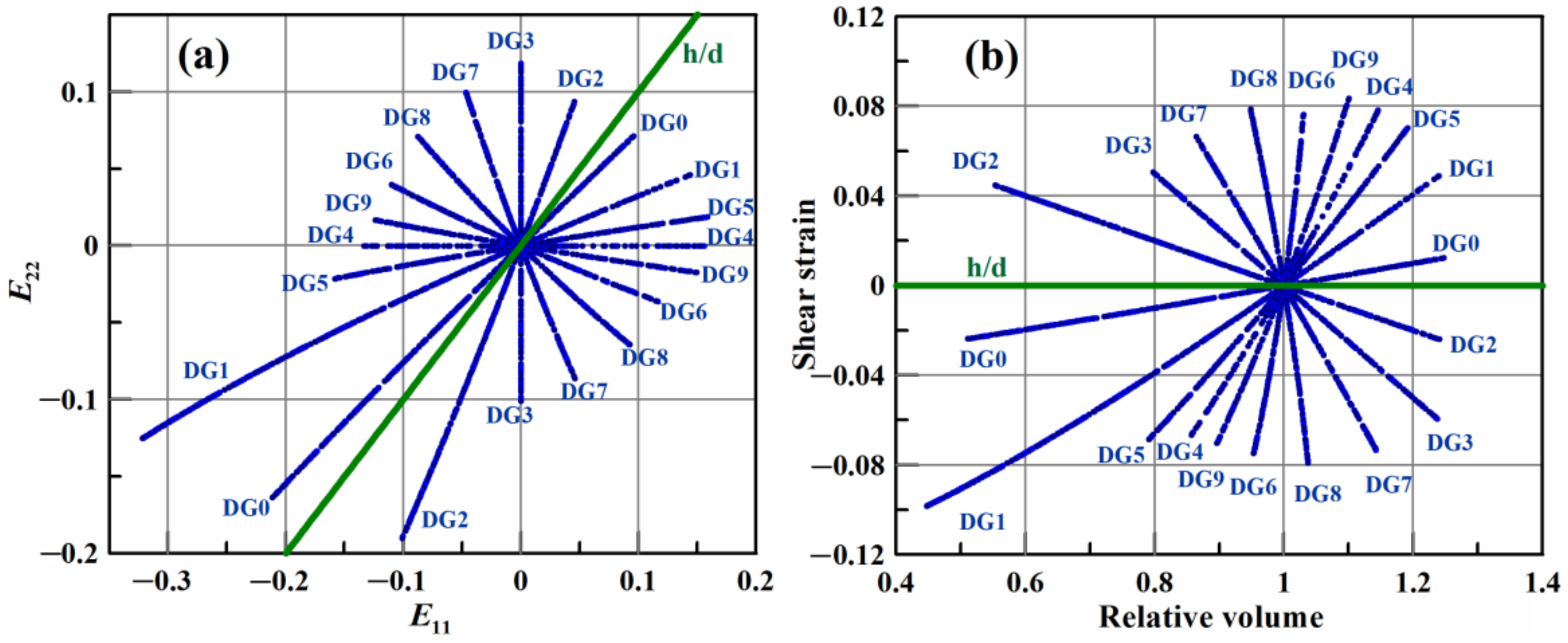
Figure 1. Deformation paths at the room temperature in the following coordinates: (a) Green–Lagrange strain tensor components E11 and E22, and (b) relative volume EV = V/V0—shear strain ES = (E11E22)/2. The green line “h/d” shows the case of hydrostatic (volumetric) deformation.
Metals 12 00402 g001
Figure 2. Room-temperature isotherm of Cu: (a) present MD simulations with EAM potential [40] in comparison with the experimental data [50] on compression in diamond anvil cell and DFT calculations [51]; (b) approximation of MD data by a sixth-order polynomial, Equation (4).
Metals 12 00402 g002
Figure 3. Data for training of the EOS ANN at room temperature: (a) shear-strain-dependent component of pressure and (b) stress deviator.
Metals 12 00402 g003
Figure 4. Evolution of shear stress, atomic structure and dislocation structure: compression along the path DG4 at 300 K. The stripes of hcp phase show the stacking faults left behind the partial Shockley dislocations.
Metals 12 00402 g004
Figure 5. Fcc–bcc phase transition in copper: (a) beginning of this transition under compression along the deformation path DG1 (b) and the pressure of bcc transition as a function of temperature for compression along several deformation paths.
Metals 12 00402 g005
Figure 6. Tensile fracture of copper: Evolution of pressure and atomic configurations for the case of tension along the deformation path DG3 at 300 K. The void surface is shown by blue surface mesh obtained by the “Construct surface mesh” algorithm of OVITO.
Metals 12 00402 g006
Figure 7. Results of ANN training for the tensor equation of state: MD data (black circles) and ANN predictions (red crosses) for (a) the pressure correction P P i , (c) the stress deviator ( S ) and (e) the correction U U i for the specific internal energy; correlation of the MD and ANN for (b) the pressure correction, (d) the stress deviator and (f) the correction of the specific internal energy, where black line shows the limit of perfect match.
Metals 12 00402 g007
Figure 8. Description of the homogeneous nucleation of dislocations in copper on the basis of trained ANNs: (a) the threshold strain states in the coordinates E V , E S ; (b) the same threshold in the strain–stress coordinates E V , S .
Metals 12 00402 g008
Figure 9. Description of the void nucleation in copper on the basis of trained ANNs: (a) the threshold strain states in the coordinates E V , E S ; (b) the same threshold in the strain–stress coordinates E S , P .
Metals 12 00402 g009
Figure 10. Description of the beginning of bcc transformation in copper on the basis of trained ANNs: (a) the strain states of the beginning of bcc transformation in the coordinates E V , E S ; (b) the same states in the strain–stress coordinates E V , S .
Metals 12 00402 g010
Figure 11. Results of Bayesian algorithm of parameter identification: contour maps of probability of model parameters: (ac) show different pairs of parameters to be identified.
Metals 12 00402 g011
Figure 12. Comparison of the MD with the dislocation plasticity model with optimal parameters determined by means of the Bayesian algorithm: strain dependencies of stress deviator for different strain paths at 300 K. Panels (af) correspond to different deformation trajectories and modes as indicated near the curves.
Metals 12 00402 g012
Figure 13. Comparison of the MD with the dislocation plasticity model with optimal parameters determined by means of the Bayesian algorithm: strain dependencies of stress deviator for different strain paths at 800 K. Panels (af) correspond to different deformation trajectories and modes as indicated near the curves.
Metals 12 00402 g013
Figure 14. Comparison of the MD with the dislocation plasticity model with optimal parameters determined by means of the Bayesian algorithm: evolution of dislocation density with applied strain at 300 K. Panels (af) correspond to different deformation trajectories and modes as indicated near the curves.
Metals 12 00402 g014
Table 1. Deformation paths studied in MD for copper single crystal with the axis of symmetry coinciding with the lattice direction [100].
IdentifierAxial Strain Rate (ns−1)Transverse Strain Rate (ns−1)
DG00.40.3
DG10.60.2
DG20.20.4
DG300.5
DG410
DG50.80.1
DG60.6−0.2
DG70.2−0.4
DG80.4−0.3
DG90.8−0.1
Table 2. Parameters of the dislocation plasticity model determined by fitting with MD by means of the Bayesian algorithm: B is the friction coefficient of gliding dislocation, α is the hardening coefficient, k m is the coefficient of efficient energy of dislocation multiplication, k n is the coefficient of nucleation barrier and k a is the annihilation coefficient.
ParameterValue
B 1.88 × 10⁻⁵ Pa × s
α 1.56
k m 1.4
k n 0.3
k a 50
Publisher’s Note: MDPI stays neutral with regard to jurisdictional claims in published maps and institutional affiliations.

