Abstract
The third generation of advanced high-strength steels (AHSS) brought attention to the steel and automotive industries due to its good compromise between formability and production costs. This work evaluated a third-generation AHSS (USS CR980XG3TM) through microstructural and X-ray diffraction (XRD) analyses, uniaxial tensile and plane-strain tension testing, and numerical simulations. The damage behavior of this steel is described with the Gurson–Tvergaard–Needleman (GTN) model using an identification procedure based on the uniaxial tensile and initial microvoids data. The microstructure of the CR980XG3TM steel is composed of ferrite, martensite–austenite islands, and retained austenite with a volume fraction of 12.2%. The global formability of the CR980XG3TM steel, namely the product of the uniaxial tensile strength and total elongation values, is 24.3 GPa%. The Lankford coefficient shows a weak initial plastic anisotropy of the CR980XG3TM steel with the in-plane anisotropy close to zero (−0.079) and the normal anisotropy close to unity (0.917). The identified GTN parameters for the CR980XG3TM steel provided a good forecast for the limit strains defined according to ISO 12004-2 standard from the uniaxial tensile and plane-strain tension data.
1. Introduction
Climate changes are becoming more and more of a central topic of global discussions. In addition to concerns about CO2 emissions, the high fossil fuel prices harm the global economy. Thus, reducing the dependence on fossil fuels by increasing the efficiency and sustainability of new passenger cars and light commercial vehicles became a priority [1]. The European Union agreed to set a reduction target of 37.5% CO2 for vehicles by 2030 with the 2021 baseline [2]. In response to the European Commission proposal, the European Automobile Manufacturers Association (ACEA) advocates a realistic target to reduce 20% of CO2 emissions [3]. In this context, the advanced high-strength steels (AHSS) have gained considerable importance in the automotive industry. This steel class has been developed to satisfy the requirements of vehicle performance and weight optimization. Several AHSS steel grades can be applied in the vehicle design, each strategically placed in the Body-in-White (BIW) to increase the crashworthiness performance. The excellent compromise between uniaxial tensile strength and elongation allows manufacturing of the BIW components with reduced thickness, producing lighter vehicles resulting in fuel economy and reducing greenhouse gas emissions.
The AHSS are commonly categorized by generation. The first generation comprises the Dual-Phase (DP), the Transformation Induced Plasticity (TRIP), Complex-Phase (CP), and martensitic (MART) steels. The second generation of the AHSS includes the Twinning Induced Plasticity (TWIP), Al-added lightweight steel with Induced Plasticity (L-IP), and the Austenitic Stainless Steel (AUST.SS). The first generation of AHSS, which has ferrite-based microstructures, is already well established [4]. Concerning the second generation, the automotive sector considers these materials attractive due to their excellent formability. However, the second generation is more expensive due to the high alloy addition required to stabilize the austenite at room temperature, mainly the Mn contents between 20 and 30 wt.%. The third generation of AHSS refers to a recent class with mechanical properties between the first and second generations and lower production costs than the second generation. These characteristics are achieved through a multiphase microstructure with a significant amount of retained austenite [5,6].
In 2003, Speer et al. [7] introduced the quenching and partitioning (Q&P) process to exploit novel martensitic steels containing retained austenite. Afterward, other steel compositions and processing routes have also been proposed within this new generation of AHSS. Among them, the Medium-Mn (MMnS), TRIP-aided Bainitic Ferrite (TBF), density-reduced (δ-TRIP), and Nanophase Refinement and Strengthening (NR&S) steels [8,9,10]. Wang and Speer [11] reported that, in 2009, the Baosteel group was the first company to process the third-generation AHSS sheets industrially. The industrial implementation of the third-generation AHSS started with the Q&P 980 1180 grades. However, there is still little information on marketable products. In 2015, General Motors (GM) announced the third generation of AHSS in the SIAC-GM’s Chevrolet LOVA RV, reducing the weight of selected body components by approximately 20%. This outcome was from a joint venture between GM Pan Asia Automotive Technical Center (PATAC), Baosteel, and the University of Tongji to introduce the third-generation AHSS in GM vehicles [12]. The U.S. Steel developed a third-generation AHSS with a 980 MPa minimum tensile strength, commercially referred to as 980XG3TM steel. The 980XG3TM steel exhibits an excellent combination of strength and ductility. According to the Japanese industrial standard (JIS), Hance and Link [13] found an ultimate tensile strength of 1017 MPa and a total elongation of 25% using the specimen Nº 5. Stamping tests were carried out with the 980XG3TM steel to manufacture components with reduced thickness for the Fiat Chrysler Automobiles [14].
The introduction of AHSS steel grades has been driven by global market requirements and increasing customer demands [15]. In principle, any steel with both ultimate tensile strength () and total elongation () within the window between the first and second generations could be a potential candidate for the 3rd generation of AHSS [16]. In terms of the and values determined from standard uniaxial tensile tests, there is still no consensus on the classification used for the 3rd generation of AHSS. Some authors establish as minimum global formability, being desirable at least and [4,9]. The U.S. Department of Energy set two targets, namely one steel grade with and () and another steel grade with and () [8]. Other authors consider performances greater than sufficient to be classified as the third generation of AHSS [17]. Most studies in the literature report AHSS steel sheets with global formability varying between 20 and 30 GPa%, which are commonly referred to as the current third generation. Figure 1 shows the global formability diagram, in which a window between the first and second generations is highlighted as an opportunity range for the development of the third-generation AHSS.
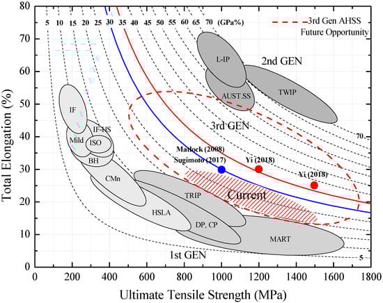
Figure 1.
Global formability diagram of various automotive steels: the future opportunity and classifications of the third generation of AHSS. Adapted from [4], data from [4,8,9].
Even though the third generation of AHSS is still in progress, some applications have already been started in the automotive sector. Its inclusion in selected parts in the BIW is expected to improve vehicle safety, fuel consumption, and drivability. Noder et al. [18] conducted a comparative evaluation between the first- and third-generation AHSS for automotive forming and crash applications. However, most of the research in the literature relating the mechanical properties of third generation-AHSS with industrial applications is focused on the structural embrittlement caused by martensitic transformation during welding processes [19,20,21,22,23].
It is crucial to understand its plastic behavior to better take advantage of the third-generation AHSS mechanical properties for sheet metal forming applications. Thus, the experimental testing procedures and modeling of this emerging steel class are necessary steps to evaluate the design of the components and verify the blank material performance in sheet metal forming operations. According to Sun et al. [24], the constitutive model proposed by Gurson [25] is the most established damage theory that describes the ductile fracture of metallic materials caused by the growth of microvoids. Afterward, the Gurson model was improved by several researchers. The extension developed by Tvergaard and Needleman [26], commonly referred to as the GTN damage model, has achieved wide acceptance by the scientific community [27]. The adequate use of the GTN in the simulation of engineering problems depends on the calibration of the nine constitutive parameters associated with the material. Generally, some very complex numerical approaches to identify these parameters are adopted, such as response surface methodology or artificial neural networks [28,29,30]. In this context, this work aims to contribute to the numerical modeling of the plastic behavior of the current third generation of AHSS with 980 grades. A simple methodology for identifying the parameters of the GTN damage model is adopted based on the uniaxial tensile data and microvoid analysis. As an outcome, the complete set of the GTN model parameters is obtained, which can reasonably reproduce the observed CR980XG3TM steel sheet plastic behavior between uniaxial tensile and plane-strain tension deformation modes.
2. Materials and Methods
The CR980XG3TM steel investigated in this work is a commercially available product being delivered to us as an uncoated cold-rolled sheet with a nominal thickness of 1.58 mm. The chemical composition and processing parameters are not given hereafter to respect the confidentiality requirements of the steel producer.
2.1. Microstructural Analysis
The microstructural characterization of the CR980XG3TM steel was performed following standard metallographic preparation procedures. The mechanical grinding, conventional polishing, followed by electropolishing using a Struers A2 electrolyte, were used to reveal the as-received microstructure. The sample preparation was completed by electrolytic polishing and etching using Struers LectroPol-5 automatic equipment operated at 35 V. The micrographs of the as-received CR980XG3TM steel were obtained with the scanning electron microscope Hitachi model SU-70.
The methodology detailed in the ASTM E975-13 standard was adopted to evaluate the volume fraction of retained austenite. The procedure is based on the analysis of X-ray diffractograms (XRD). The method can be applied to carbon and alloy steels with a near-random crystallographic orientation of the phases. The retained austenite volume fraction is calculated as:
where and denote, respectively, the austenite (-iron: face-centered cubic) and ferrite plus martensite (-iron: body-centered cubic). In Equation (1), is the integrated intensity per angular diffraction peak, whereas is a parameter that depends upon the interplanar spacing (), the Bragg angle , the crystal structure, and the composition of the phase being measured. The XRD measurements were performed in the Rigaku SmartLab (Rigaku Corporation, Tokyo, Japan) X-ray diffractometer with a Cu tube, and K-alpha radiation operated at 40 kV and 30 mA using a scanning range from 40° to 110° with a scan speed of 2°/min. The values of and can be calculated from basic principles [31].
2.2. Mechanical Testing
The mechanical properties of the CR980XG3TM steel sheet were assessed from uniaxial tensile tests. The digital image correlation (DIC) system manufactured by GOM coupled with the ARAMIS-5M software (GOM GmbH, Braunshweig, Germany) measured the strain fields. The specimens were manufactured by CNC (Computer Numerical Control) milling machining MIKRON VCE 500 (Mikron Machining, Agno, Switzerland) from guillotined sheet strips. The dog-bone specimen dimensions are depicted in Figure 2.
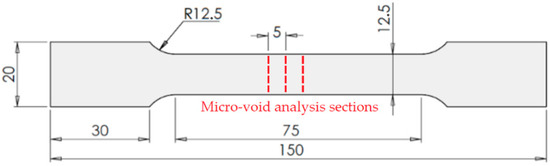
Figure 2.
Geometry, dimensions (mm) of the uniaxial tensile test specimen, and slices cut from the gauge length region for the void formation analysis.
The gauge length of 50 mm in the central specimen region was used as the reference image for DIC measurements. For this purpose, a high contrast stochastic (speckle) pattern was adopted by first applying a matte white aerosol ink to prepare the specimen background surface. Then, after a drying time of about 10 min, a matte black ink was sprayed over the white background. The uniaxial tensile tests were performed after the painting, about 30 min of curing. To evaluate the in-plane sheet anisotropy, the uniaxial tensile tests were performed at three angular orientations to the sheet rolling direction (RD), namely 0°, 45°, and 90°. Five replicas were tested for each angular orientation. The tests were carried out up to fracture at room temperature (20 °C) using the universal testing machine Shimadzu AG-X 100 kN (Shimadzu, Kyoto, Japan), under a constant crosshead speed of 4.5 mm/min, corresponding to a nominal strain rate of 10−3 s−1. The strain measurements were recorded with an image acquisition rate of 1 frame/s.
Double-notched specimens with a radium of 1 mm were adopted to assess the plane-strain tension mode. Figure 3 presents the specimen geometry. The universal testing machine Shimadzu AG-X 100 kN with a 0.1 mm/min crosshead speed was employed. The specimen preparation procedures for evaluating the strain field are the same as described above for the case of uniaxial tensile test samples. Uniaxial tensile and plane-strain specimens were used to obtain the limit strains. The limit strains were defined from the specimens taken at the rolling and transverse sheet directions in both deformation modes. According to the ISO 12004-2 standard [32], the principal limit strains were defined as the average values determined from three replicated tests for each deformation mode and specimen angular orientation to the rolling direction.
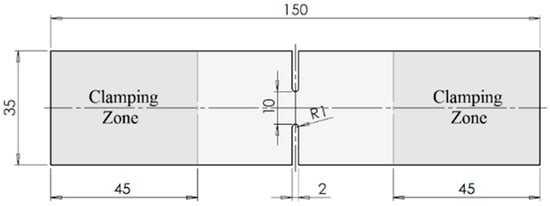
Figure 3.
Plane-strain tension specimen geometry and dimensions (mm) [33].
2.3. Microvoid Analysis
Interrupted uniaxial tensile tests were used to analyze the formation of voids resulting from the imposed straining level. Three increasing longitudinal true-strain levels were selected: 0% (as received), 13%, and the fractured condition. The uniaxial tensile tests were performed in specimens taken at the rolling direction using a crosshead speed of 4.5 mm/min. After the uniaxial tests, the samples were cut from the gauge length region in slices with 5 mm length; see the red cross sections shown in Figure 2. The slices were cut using a precision metallographic cutter by applying a low cutting feed and high cooling. Then, the sliced pieces were mounted into epoxy resin and mechanically prepared with SiC abrasive grinding papers 180, 240, 600, 800, 1200, and 2400-grit using a Struers TegraPol-2 machine (Struers, Tokyo, Japan). The polishing was performed in two steps by applying a diamond paste of 6 and 3 microns, respectively.
The uniaxial tensile samples were analyzed in the scanning electron microscopy (SEM) Hitachi TM4000Plus (Hitachi, Tokyo, Japan). Three sections were analyzed for each uniaxial tensile straining level. Twenty images were taken for each section, resulting in 60 images for each straining level. The ImageJ open-source software with the “Analyze Particles” function was employed in the quantitative analysis of microvoids to determine the measures of the void area fraction, defined as [34]:
2.4. GTN Damage Model Parameters Calibration
The GTN damage model, proposed initially by Gurson [25] and later extended by Tvergaard and Needleman [26], is widely used to describe the micromechanical damage effects of ductile metals. The GTN damage model is defined by following the yield function:
With
where is a critical value of void volume fraction, and is the void volume fraction at fracture. In Equation (6), , , and are the yield locus parameters, whereas is the damage parameter defined by Equation (7). The GTN model is an extension of the von Mises isotropic yield function accounting for the effects of the hydrostatic pressure on the plastic yielding of metals. In Equation (6), is the von Mises equivalent stress measure defined from the components of the deviatoric stress tensor:
In which is the Cauchy second-order stress tensor, is the hydrostatic stress component, and is the second-order identity tensor. In Equation (6), is the stress triaxiality factor defined by the ratio between the hydrostatic stress and the yield stress of the fully dense matrix material, that is, . In the GTN model, the damage arises partly from the growth of existing microvoids and the nucleation of new voids by cracking or from the interface decohesion of inclusions and precipitates at the material matrix. The damage evolution in the GTN model is written in terms of an additive rate decomposition considering the contributions of both void growth (VG) and nucleation (VN) as:
In which
In Equation (9), stands for the plastic strain-rate second order while is the equivalent plastic strain rate. In Equation (10), is defined by a nucleation plastic strain which follows a normal strain distribution with an average plastic strain value and a corresponding standard deviation . The parameter is the void volume fraction of nucleating particles. The damage material behavior using the GTN model is entirely defined by three material parameters (, , ), three void nucleation parameters (, , ), two failure parameters (, ), and the initial relative density which is obtained from the initial porosity, .
The adopted procedure is firstly cast by assuming that the effective plastic behavior of the material matrix is fully dense, namely with no initial voids. Thus, the work-hardening equations describing the experimental plastic behavior can be corrected using the effective stress measure concept defined from the uniaxial tension load [35]. The effective stress concept is schematically depicted in Figure 4a by a representative volume element (RVE) in which is the uniaxial load, whereas and stand for the overall section and the voided areas of the RVE, respectively. In this way, the effective stress measure is obtained as:
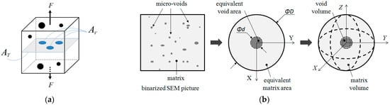
Figure 4.
(a) Representative volume element (RVE): effective stress measure and (b) definition of the initial void volume fraction from the measured void area fraction [36].
In Equation (11), is the fraction area of voids, and is the true stress which can be defined from the work-hardening equations () fitted to the experimental uniaxial tensile curve at the rolling direction. Moreover, is viewed as a scalar variable by assuming isotropic damage conditions. The voids are supposed to be equally distributed in the matrix and independent of the loading path.
Secondly, from the average measured values of the voided area fraction as a function of the total longitudinal true strain in uniaxial tension at the sheet rolling direction, and neglecting the elastic strains, a linear relationship is adopted to describe the voided area fraction with the true plastic strain as:
The initial porosity parameter of the initial void volume fraction was obtained from an RVE, which is assumed to be equivalent to the binarized image determined from SEM analysis, as schematically depicted in Figure 4b. This RVE is composed of a small single spherical void embedded concentrically in a large spherical metal matrix. The spherical matrix has a diameter , whereas the spherical single void has a diameter , which, in turn, is assumed to be equivalent to the actual binarized SEM areas of the material matrix and voids, respectively. The initial void volume fraction () can thus be estimated from the initial area of voids () represented by the intercept of Equation (12), that is:
For steels, the typical values of the GTN yield locus parameters in Equation (6) are , , and [26]. The parameter affects the load-bearing capacity of the material, namely provides a decrease in yield strength leading to a material softening due to void growth to the detriment of the matrix material’s work hardening. The second GTN yield locus parameter is associated with the stress triaxiality factor in the GTN yield function, , which depends on the hydrostatic stress and the material yield strength. This work adopted the calibration results of the micromechanical modeling developed by Faleskog et al. [37].
The nucleation of new voids in the GTN model is controlled by the equivalent plastic strain rate with a probability density function, which follows a normal distribution, Equations (9) and (10), and depends on the calibration of three parameters (, , ). The parameter is a mean value of characteristic nucleation plastic strain and corresponds to its standard deviation. The parameter is the volume fraction of the nucleated voids. The following ranges of values are reported in the literature for typical metals: = 0.1–0.3, = 0.05–0.1, and = 0.01–0.05 [28]. In this work, the calibration of the nucleation parameters of the CR980XG3TM steel was performed by finite element simulations of the uniaxial tensile test. Here, the idea is to vary the set of parameters to obtain a predicted nominal stress–strain curve close to the experimental uniaxial tensile test results, including post-necking behavior. Figure 5 shows the schematic geometrical model proposed to simulate the uniaxial tensile test. The simulation test was conducted by fixing one grip section and applying a prescribed constant speed at the other grip section. The quasi-static numerical simulations were performed with the ABAQUS/explicit commercial finite element code, wherein the GTN model is available as porous metal plasticity. In all numerical simulations, the specimen has meshed with the C3D8R element type: 8-nodes linear brick, reduced integration, and hourglass control [38]. The functionality Element Deletion was selected in the finite element ABAQUS mesh module. This option removes the finite element when it loses the strength capacity completely.
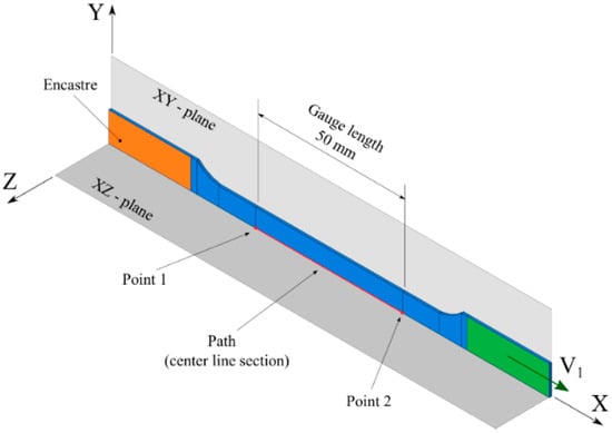
Figure 5.
Boundary conditions for the uniaxial tensile specimen with 1/4 symmetry.
Once the nucleation parameters are determined, it is possible to produce numerical predictions for the uniform domain. These numerical predictions and experimental measurements obtained through the uniaxial tensile test were used to calibrate the failure parameters. To determinate the critical value of the void volume fraction (), an image of the major strain field obtained from the uniaxial tension specimen immediately before the fracture was used as a reference. A critical region in the localized necking and another area located sufficiently far from the necking was monitored from finite element simulation and compared with the experimental result. To identify the parameter , two experimental results were considered, namely the endpoint of the elongation–force curve and the width reduction in the specimen after the fracture.
3. Results
3.1. As-Received Microstructure
From the analysis conducted by Finfrock et al. [39] for Q&P steels and the martensitic structure characterization performed in the work of Navarro-Lopez et al. [40], the dark regions in Figure 6b are ferrite (F) and the fine internal laths surrounded by white blocks are martensite–austenite islands (MA). In contrast, the elongated white regions are the retained austenite (RA). According to Wang and Speer [11], the main alloy elements of Q&P 980 steel are C, Mn, and Si, with nominal values ranging between 0.20–0.25, 1.50–2.40, and 1.2–1.6%, respectively. Other elements such as Al, P, and S could also be found in residual amounts. The microstructure of commercial Q&P steels is primarily composed of martensite (50–80%) formed during the quenching process, ferrite (20–40%) resulting from the austenitic phase during slow cooling, and the dispersed retained austenite (5–10%), which, in turn, is stabilized by the carbon enrichment during the partitioning step [11].
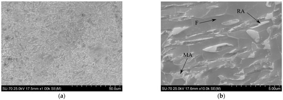
Figure 6.
SEM micrographs of the as-received CR980XG3TM steel sheet with (a) 1000× and (b) 10,000× highlighting the ferrite (F), martensite–austenite (MA), and retained austenite (RA).
The X-ray diffractogram of the CR980XG3TM steel for the as-received condition is shown in Figure 7, in which the peaks are identified as -iron or -iron.
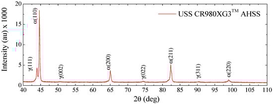
Figure 7.
X-ray diffractogram patterns from the as-received CR980XG3TM steel.
Table 1 presents the calculated and values for Cu radiation and the integrated intensity per angular diffraction peak. Each peak was fitted with the Lorentz fit peak tool available in the OriginLab software. From Equation (1) and Table 1 data, the estimated volume fraction of the retained austenite in the present CR980XG3TM steel sheet is 12.2%, which was very close to the value of ~12% reported for the Q&P 980 steel [19,20].

Table 1.
Theoretical and using Cu radiation (data from [41]) and integrated intensity per angular diffraction.
3.2. Mechanical Properties
The average elastic properties of the CR980XG3TM steel determined in the rolling direction are the Young modulus, = 195 ± 5 GPa, and Poisson’s ratio = 0.289 ± 0.003. The plastic behavior of the CR980XG3TM sheet was evaluated from the yield stress defined at 0.2% of the plastic-strain offset (), ultimate tensile strength (), uniform elongation (), total elongation (), and Lankford’s anisotropy coefficient (-value). The -value was defined as the slope between the width and the thickness strains between yield strength and the maximum uniform plastic strain values. Table 2 resumes the average mechanical properties of the CR980XG3TM steel as a function of the angular orientation and the corresponding standard deviation values.
Table 2.
The uniaxial tensile properties of the CR980XG3TM steel.
The CR980XG3TM steel is classed as a current third-generation AHSS, as shown in Figure 8. Its ultimate tensile strength (1040 MPa) and total elongation (23.4%) allow reaching 24.3 GPa% as performance in the global formability diagram, which is close to the Q&P results reported in the literature [11,19,20,39]. The quenching and partitioning steels are still under the desired performance target, namely 30 and 35 GPa% (Figure 1). However, they significantly outperform the well-established first-generation AHSS, such as DP and TRIP.
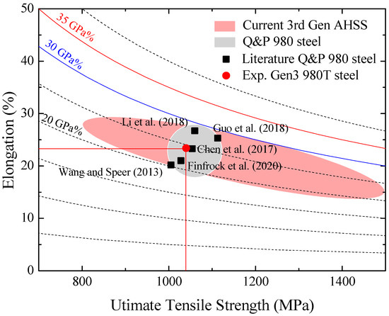
Figure 8.
Placement of the investigated CR980XG3TM steel in the global formability diagram. Data from [11,17,18,22,23].
From Table 2, the planar and normal anisotropy coefficients are obtained, respectively, and . At first glance, the uniaxial tensile plastic behavior of the investigated CR980XG3TM steel sheet can be regarded as isotropic given that the values found for and are close to zero and unity, respectively. However, in Figure 9a, one can observe deviations in the uniaxial tensile engineering stress–strain behavior at 0°, 45°, and 90° in-plane angular orientations. Figure 9b further emphasizes this observed anisotropic behavior wherein the CR980XG3TM steel would present small amplitudes of earing formation in the cup-drawing test. The formability of the CR980XG3TM steel is close to that of DP600, with higher strength. Figure 9c shows the yield stress and strength values normalized by the corresponding data at the rolling direction. The yield stress behavior presents a monotonic increase of about 11% between 0° and 90° orientations, whereas the ultimate tensile strength varies by less than 5%.
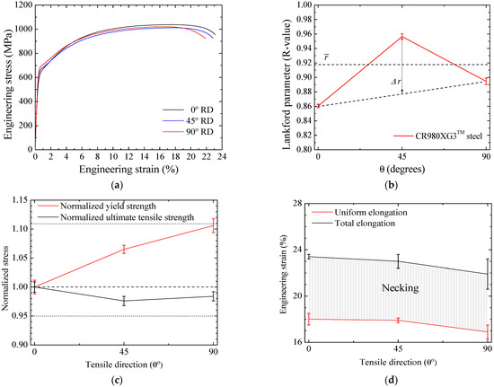
Figure 9.
Uniaxial tensile test results of the CR980XG3TM steel sheet: (a) engineering stress–strain curves at 0°, 45°, and 90°, and angular evolutions of the (b) Lankford r-values, (c) normalized yield stress and ultimate tensile strength, and (d) uniform and total elongation.
Conversely, the average uniform and total elongation values and corresponding standard deviations are depicted in Figure 9d. A slight reduction between the sheet rolling and transverse directions is observed in both uniaxial uniform and total elongation values. Moreover, the average engineering strain amount during the post uniform uniaxial tensile behavior shows minor variation, as indicated by the shaded area in Figure 9d.
The uniaxial tensile plastic behavior at the rolling direction of the CR980XG3TM steel sheet was fitted according to the Hollomon, Ludwik, Swift, and Voce work-hardening equations. Table 3 presents the average values of the fitted work-hardening parameters along with the corresponding goodness-of-fit (R2) values. The Ludwik work-hardening equation corresponds to the first term of the Johnson–Cook plasticity model, which is widely adopted in finite element simulations [42]. Alternatively, the pre-strain term in Swift’s equation can be used to describe the initial plastic yielding or a prior deformation process as, e.g., from a cold-rolling skin pass. The best fits were obtained with the Swift and Voce work-hardening equations with R2 equal to 0.996 and 0.999, respectively.
Table 3.
Parameters of the work-hardening equations of the CR980XG3TM steel sheet determined from the uniaxial tensile tests performed at the rolling direction.
3.3. Limit Strains
Figure 10 shows the major and minor true total-strain fields in the gauge length of the uniaxial and plane-strain tension specimens obtained before the fracture. The average principal limit strain values and corresponding standard deviations for both uniaxial and plane-strain tension deformation modes are resumed in Table 4. The limit strains obtained from the uniaxial tension tests are close at the rolling ( deg) and transverse ( deg) directions. The corresponding in-plane strain ratio at an angular orientation to the sheet rolling direction, , , that is equal to −0.4568 and −0.4656 for and 90 deg, respectively. These values are also very close to the theoretical in-plane strain ratios that can be defined from the normal anisotropy coefficients listed in Table 4. From the Lankford r-value definition, by assuming plastic incompressibility, it is obtained under a proportional strain path that The latter gives the in-plane strain ratio, respectively, equal to −0.4626 and −0.4723 for the rolling and transverse angular orientations.
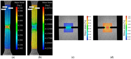
Figure 10.
DIC measurements during the in-plane tests: (a) major strain and (b) minor strain fields obtained from the uniaxial tension specimen, and the selected (c) major strain and (d) minor strain fields from the double-notched plane strain specimen.
Table 4.
Limit strains of the CR980XG3TM steel sheet determined from the in-plane tests.
3.4. Void Results
The polished surface of the as-received sample is shown in Figure 11a, and the corresponding binarized image is depicted in Figure 11d, wherein the black regions represent the voids. Figure 12 exhibits the void area fraction values obtained from Equation (2), ranging from 0.1 to 0.5%. The void density, mean void size, and the void aspect ratio determined from Equations (2)–(5) are also presented in Figure 12.
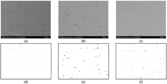
Figure 11.
SEM micrographs (1500×) and corresponding binarized image of CR980XG3TM steel sheet in (a,b) as received, (c,d) 13% true strain, and (e,f) fractured condition.
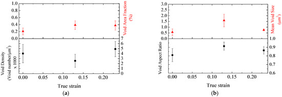
Figure 12.
Void analysis results: (a) void density and void area fraction, (b) void aspect ratio and mean void size.
3.5. Full Set of GTN Damage Model Parameters
3.5.1. Effective Work Hardening and Initial Porosity
Figure 13a shows the linear fitting results determined from the experimental average void area fraction of the CR980XG3TM steel sheet. The corresponding and values in Equation (12) are also indicated in Figure 13a. The predicted stress–strain curves of Swift and Voce work-hardening equations obtained from Equation (11) are compared with the experimental true-stress and true plastic strain in Figure 13b. Both work-hardening equations show good agreement with the experimental uniaxial tensile behavior observed in the uniform plastic-strain domain. Despite presenting a better fit, Voce’s equation provides saturation of the work hardening for larger strains. Using the GTN damage model, such plastic behavior will rapidly lose the load-bearing capacity at the necking onset. In this way, the Swift work-hardening equation was selected to describe the behavior of the fully dense matrix since it provides a better fit to the experimental stress–strain data when considering the softening effect. From the result presented in Figure 13a and Equations (12)–(14), the initial porosity was estimated as: .
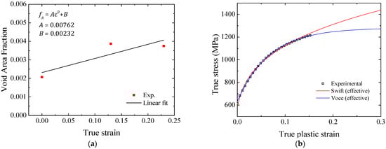
Figure 13.
(a) Experimental void area fraction as a function of the true longitudinal plastic strain obtained for the CR980XG3TM steel sheet under uniaxial tension concerning the rolling direction and (b) comparison between the experimental true-stress and true plastic-strain data and the predicted work-hardening curves in the rolling direction.
3.5.2. Yield Locus Parameters (, , )
From micromechanical simulations considering unit cell finite element models with a homogeneous material and a single spherical void, the former described by the GTN model, Faleskog et al. [37] proposed a procedure for the yield locus parameters calibration, revealing that (, ) parameters exhibited a dependence on the strain-hardening exponent () and the ratio between the yield strength () and Young’s modulus (). This procedure is adopted here to define these GTN yield loci parameters avoiding extensive experimental and or combined numerical investigations given the non-uniqueness of the GTN damage model parameters. From the calibration results of the micromechanical modeling developed by Faleskog et al. [37], the parameters (, ) are obtained as a function of the average strain-hardening exponent and the ratio between the yield stress and the Young modulus, . Thus, the yield locus parameters found for the CR980XG3TM steel sheet are , , and .
3.5.3. Void Nucleation Parameters (, , )
The parameter produces a softening of the plastic behavior. Considering the values of , , to be fixed, increasing the -value produces a more significant softening effect [38]. Table 5 presents the parameters used to simulate the elastoplastic behavior of the fully dense material. The total reaction force was obtained by summating the fixed region nodal reaction forces (the orange area in Figure 5) multiplied by four to account for the two planes of symmetry. The specimen elongation was calculated from the difference in displacements of points 1 and 2, indicated in Figure 5.
Table 5.
Elastic properties and parameters of the isotropic effective work hardening.
Figure 14 compares the experimental and predicted displacement–force determined using the parameters listed in Table 5. The current numerical results overpredict the experimental data, mainly the post-necking elongation up to fracture. From the typical values for metals presented in the literature, several combinations of , , were tested, aiming to describe the post-necking displacement–force curve. The set of nucleation parameters that provided the best fit is listed in Table 6. The softening resulting from the nucleation parameters can be observed in Figure 14.
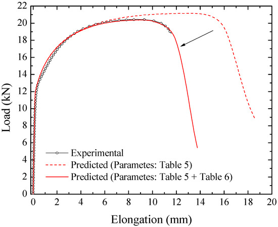
Table 6.
Initial porosity, material, and void nucleation parameters.
3.5.4. Failure Parameters (, )
To determinate the critical value of the void volume fraction (), Figure 10a was used as a reference. The picture shows the major strain field immediately before the fracture in the uniaxial tension mode. According to the digital image correlation analysis, the maximum longitudinal total strain reached before the fracture onset is = 0.54. Two specimen regions were monitored from the finite element simulation calibrated with the GTN nucleation parameters, see Figure 14. One region is the critical region in the localized necking, and the other is located at a distance sufficiently far from the necking, shown in Figure 15a. The plot in Figure 15b shows that, as expected, up to the necking onset, all the elements of the gauge length deform uniformly. After starting the necking, the strain far from the necking remains almost constant while the strain at the necking zone increases rapidly. Thus, once the necking begins, only the specimen central region increases elongation, and the failure parameters must be calibrated from this region.
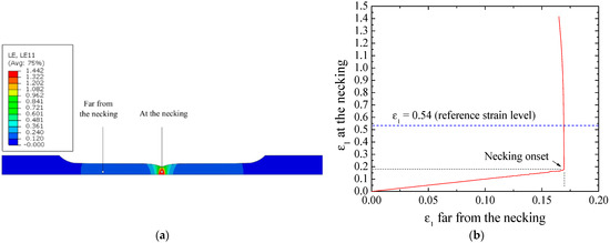
Figure 15.
Major strain predictions of the uniaxial tensile test without the failure parameters: (a) regions at the necking and far from the necking and (b) corresponding major strain history.
Figure 16 resumes the methodology for selecting the parameter from the major strain value. The major strain field is observed along the specimen gauge length at the time where the maximum value is equal to = 0.54 in the necking region, Figure 16a. Figure 16b shows the value of the void volume fraction for the same time. The void volume fraction (VVF), the nucleation (VVFN), and void growth (VVFG) contributions are plotted in Figure 16c as a function of the major strain. From the major strain = 0.54, the critical void volume fraction was found equal to 0.05.
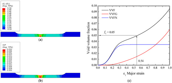
Figure 16.
Proposed identification procedure for the critical void volume fraction -value: contours plots of the (a) major strain and (b) void volume fraction, and (c) void volume fraction measures as a function of the major strain in the necking region.
The parameter denotes the void volume fraction after the complete specimen fracture. From the critical value, , the void fraction increases rapidly through the void coalescence until the value, and then, the corresponding finite element is deleted from the mesh of the uniaxial specimen model. The coalescence is governed by Equation (7) in the GTN damage model. The -value must be greater than the parameter and is limited to unity, that is, 100% voids.
To identify the parameter , two experimental results were considered. Firstly, the endpoint of the elongation–force curve. Secondly, the width reduction in the specimen after the fracture. Figure 17 shows a sequence of three different moments in the uniaxial tensile test, namely (a) undeformed, (b) localized necking before the fracture, and (c) specimen after the fracture. The width of the specimen in the fractured region measures approximately 9.80 mm, and the value of the failure parameter that best fits the experimental results for the CR980XG3TM steel under the uniaxial tension deformation mode was = 0.095. Thus, the identified parameters of the GTN damage model are presented in Table 7.
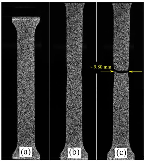
Figure 17.
Images of the uniaxial tensile specimen during the testing at (a) the unloaded state, (b) immediately before the fracture, and (c) after the fracture.
Table 7.
Full set parameters of the GTN damage model for the CR980XG3TM steel.
The contour plot predictions of the void volume fraction determined using the complete set of the GTN model parameters are shown in Figure 18a. Figure 18a depicts one of the experimental samples placed with the final predicted model shape. Moreover, the load–elongation curves showed similar results, see Figure 18b. The predicted curve is higher than the experimental data in the elongation range, close to the yielding point up to ~3 mm elongation. It may be attributed to the work-hardening description.
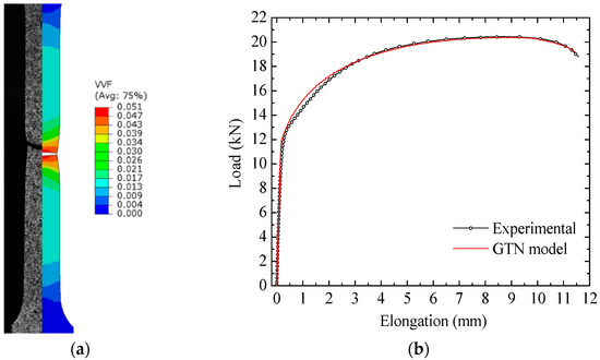
Figure 18.
(a) Finite element simulation of the uniaxial tensile test: experimental digital image and predicted deformed specimen, and (b) experimental uniaxial tensile test load elongation and predicted results obtained with the full set parameters of the GTN damage model for the CR980XG3TM steel.
3.5.5. Mesh Sensitivity
The influence of the mesh size in predicting the uniaxial tensile test was evaluated using the GTN model parameters given in Table 7. Four different mesh sizes in the specimen gauge length region were considered, namely 1.6, 0.8, 0.4, and 0.2 mm, as shown in Figure 19.
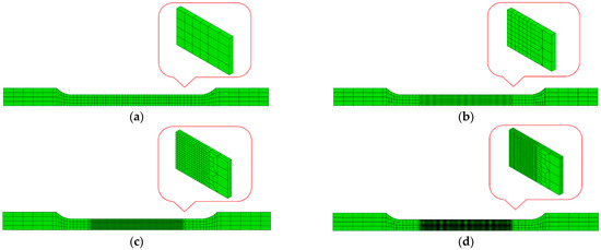
Figure 19.
Different mesh sizes in the gauge length region of the uniaxial tensile specimen: (a) 1.6 mm, (b) 0.8 mm, (c) 0.4 mm, and (d) 0.2 mm.
Figure 20 compares the force-elongation prediction determined with different mesh sizes with the experimental data to the rolling direction. The four mesh sizes provided the same behavior until the beginning of the necking. For the post-necking curve, except for the 1.6 mm mesh that exceeded the experimental curve by approximately 0.5 mm in elongation, the other finite element mesh size showed very close values, as shown in Figure 18b, were obtained with a mesh size of 0.4 mm. According to Slimane et al. [43], who conducted a parametric study of the GTN model, the numerical prediction does not have a significant mesh size dependence in the uniform plastic behavior. During the uniform elongation, the whole elements in the specimen gauge length have the same strain level. However, only a few elements continue to deform in the fracture zone from the necking point. Thus, the macroscopic behavior prediction of the uniaxial tensile test becomes dependent on the element mesh size. A fine mesh triggers the void formation faster than a coarse mesh.
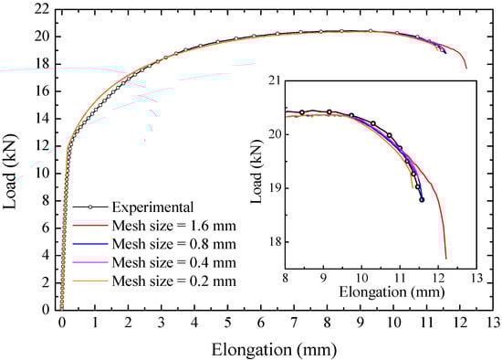
Figure 20.
Influence of the mesh size on the load–elongation curve.
The minimum standard error () was adopted to calculate the difference between the experimental and predicted results, Equation (15). The is calculated for common values of the numerical prediction and the experimental result of load–elongation of the uniaxial tensile specimen. As there is no dependence on the mesh size for the curve before the necking, the values were very close. The mesh size of 0.4 mm shows less error among the other mesh sizes concerning the experimental data. Moreover, it presented a good number of elements for its CPU time. Although the 0.8 mm mesh can represent the material’s behavior, its coarse mesh can mainly provide a poor numerical forecast in the thickness direction. Table 8 shows the minimum standard error found for each mesh size, as well as the CPU time and the number of elements, both normalized by the 1.6 mm case.
Table 8.
Mesh sensitivity—minimum standard error of load–elongation curve, CPU time, and the number of elements.
3.6. Numerical Predictions of the In-Plane Limit Strains
Using the full set parameters of the GTN damage model, finite element simulations of the flat specimens were performed. Concerning the limit strains obtained from the uniaxial tension mode, the evaluation was carried out in the experimental testing by applying the ISO 12004-2 standard. As in the experiments, these strains were analyzed along the sections in the specimen gauge length. Both experimental data obtained at 0° and 90° to the rolling direction are compared to the numerical prediction, Figure 21a. The Lankford r-values are close to unity, thus justifying the isotropic assumption made in this work. The calibrated GTN parameter for CR980XG3TM steel provided a good agreement with the experimental strains determined at 0° and 90° angular orientations. Figure 21b shows the limit strain predictions for uniaxial tension. The predicted major limit strain equals 0.346, while the minor limit strain is −0.164. For comparison purposes, the corresponding average experimental limit strain values, listed in Table 4, obtained for the specimen at the rolling direction, are 0.324 and −0.148, respectively.
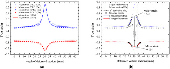
Figure 21.
(a) Experimental and predicted major and minor strains at the centerline section of the uniaxial tensile specimen, and (b) limit strains from the uniaxial tensile test simulations using the GTN model.
The finite element simulation of the plane strain with a flat double-notched specimen was also performed using a 3D mesh with C3D8R elements. The boundary conditions were like those used in the uniaxial tension model. Figure 22a shows the mesh used in the flat double-notched specimen, in which the zoomed region displays the refined elements with a mesh size of 0.4 mm. The mechanical behavior response using the GTN model was compared with the experimental results in terms of the stress–strain curve. The graph shows the experimental values with samples manufactured at 0° and 90° of the rolling direction and the stress–strain curve obtained through the finite element model. Although the calibration of the GTN model parameters was made from the uniaxial tensile test, it was observed that the selected parameters provided a mechanical behavior close to the experimentally determined values for the plane-strain tension test. The predicted stress behavior is about 2% higher than the experimental stress values. Regarding the true strain, the corresponding prediction is slightly beyond the value recorded experimentally, as shown in Figure 22b.
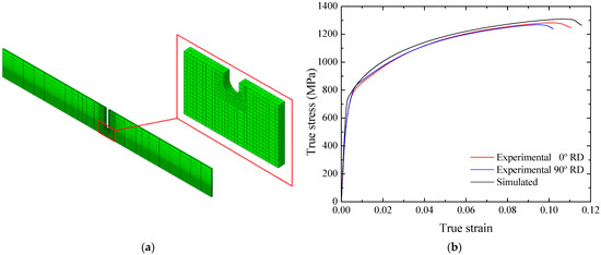
Figure 22.
(a) Mesh refinement adopted in the flat double-notched specimen, and (b) experimental true stress–strain curve of the plane strain test and predicted results obtained with the complete set of parameters of the GTN model.
Regarding the limit strains for the plane strain condition, the major strain determined from the GTN model was equal to 0.123, and the minor strain equal to 0.012. The values obtained experimentally for the major and minor strain were 0.152 and 0.011 along the rolling direction and 0.134 and 0.010 for the case perpendicular to the rolling direction. Figure 23a compares experimental and predicted major and minor strain along the specimen’s centerline, while Figure 23b exhibits limit strains calculated according to the ISO 12004-2 standard for the plane strain.
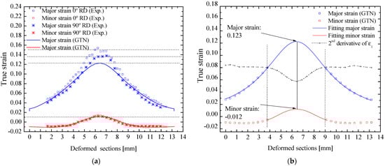
Figure 23.
(a) Experimental and predicted major and minor strain in the centerline of the double-notched plane-strain sample and (b) limit strains from the plane-strain tension test simulations using the GTN model.
The results of limit strains presented in Figure 21 and Figure 23 can also be expressed according to the concept of forming limit curve (Figure 24), in which below the curve is a safe forming condition. In this case, a safe region means the absence of necking. The predicted limit strains for the left side of the forming limit diagram reasonably agreed with the corresponding experimental data. In this sense, the proposed methodology can be applied to describe the CR980XG3TM steel sheet behavior under sheet metal forming processes conditions with .
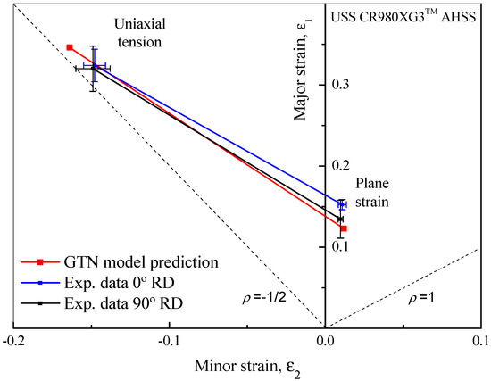
Figure 24.
Comparison between the experimental left-hand side of the forming limit curve and the numerical prediction determined for the CR980XG3TM steel sheet using flat specimens and the GTN model.
4. Discussion
In this work, the third-generation AHSS CR980XG3TM steel was evaluated using mechanical tests and microstructural analysis to calibrate the parameters of the GTN damage model. The numerical predictions of limit strains showed that the selected GTN model parameters provided a similar behavior to the experimentally observed results, representing the left side of the forming limit curve. This good agreement can be ascribed to the low planar anisotropy behavior of the CR980XG3TM steel. In this context, the methodology proposed in this work proved to be capable of predicting the macro-mechanical behavior of a recent third-generation AHSS. Many researchers in the literature have already introduced important extensions to the GTN damage model, some more widespread and adopted than others. According to Bergo et al. [44], contributions aimed at solving the GTN model’s limitation of correctly predicting material failure under low stress triaxiality, as well as extensions related to incorporating different microvoid features, such as the shape, orientation, and rotation, have been added to the GTN model by several authors in the last 20 years.
Conversely, most of these extensions increase the complexity of determining the parameters of the GTN model, either by introducing new parameters or by using more sophisticated experimental devices and calibration methods, such as tensile tests with in-situ 3D X-ray microtomography [45,46,47] and parameters identification using artificial neural networks [24,28,29,48], respectively. The model used in this work does not consider these extensions of the GTN model. The adopted modeling also does not include the strain-induced martensite transformation, which might occur in the investigated current third-generation AHSS, nor the contribution of each phase for strength and formability analyses.
Regarding the microvoids analysis, some remarks regarding the proposed methodology should be addressed. Firstly, the void area fraction analysis requires exhaustive laboratory work obtained from the treatment of several micrographs. In practical terms, only three strain levels were selected: as-received material, fractured condition, and an intermediate straining stage to assess the trendline. The straining level obtained from the fractured state (23% engineering strain) is still considered low to determine the void area fraction owing to the resulting narrow region of the localized necking. Using notched specimens, Saeidi et al. [49] observed the more significant void area fraction at higher equivalent straining levels in dual-phase (ferrite-martensite) steel. Secondly, the void analysis results were used only to define the initial void volume fraction and to forecast the plastic behavior of the completely dense material. Moreover, it is worth observing that the necking instability increases the stress triaxiality factor in the fracture region. The level of localized strain in the uniaxial tensile tests was obtained employing DIC measurements, which, together with the specimen width measurements after fracture, were used to determine the GTN model failure parameters in Section 3.5.4. Complementary void data were also presented, including void density, aspect ratio, and average size. The void analysis technique used in this work has a qualitative value since a different specimen was employed for each straining level. Therefore, it was not possible to follow the evolution of a group of microvoids. As the void measurements were performed in the specimen’s cross-section, the growth of voids was not observed along the specimen loading direction, which is usually viewed in the literature as an ellipsoid shape [50]. The proposed methodology is based on a spherical void in which volume fraction is estimated from the void area measurements of 2D micrograph images. For this reason, these experimental results were applied only to determine the initial void volume fraction, which corresponds to the undeformed condition.
The classical GTN damage model considers the void contributions related to the growth of existing voids and the nucleation of new voids. The GTN void nucleation follows a normal distribution, and its accumulated equation tends to the saturated value of , which was calibrated in Section 3.5.3 with and to describe the observed behavior of uniaxial tensile load-elongation data. According to the GTN model, only the stress triaxiality influences the void growth. It should be observed that the parameters of the GTN model were calibrated from the uniaxial tensile data at the sheet rolling direction. Thus, the corresponding limit strain predictions are close to the experimental values of the uniaxial tension deformation mode. On the other hand, this work showed that the GTN complete set parameters determined by the proposed methodology provide a reasonable forecast for the plane-strain tension mode. In this context, the set of the selected GTN parameters provides conservative predictions of the in-plane limit strains for the CR980XG3TM steel between the uniaxial and plane-strain tension deformation modes.
5. Conclusions
This work evaluated the uncoated cold-rolled CR980XG3TM steel sheet from mechanical tests and finite element modeling. The material presented a global formability = 24.3 GPa% within the region known as the current third-generation advanced high-strength steels. This excellent formability results from its multiphase microstructure composed of martensite, ferrite, and retained austenite. From the performed testing procedures and proposed finite element modeling, the main conclusions are summarized as follows:
- The standard mechanical testing provided the average mechanical properties, namely the yield stress (604 MPa), ultimate tensile strength (1040 MPa), and total elongation (23.4%). The tested material presents a weak initial plastic anisotropy, with a planar anisotropy close to zero (−0.079) along with the normal anisotropy coefficient close to unity (0.917).
- In the as-received state, the XRD analysis provided a retained austenite volume fraction of 12.2%, which, in turn, is prone to transform into martensite during the early stages of plastic straining.
- The CR980XG3TM steel provided an experimental Lankford r-value close to the unity, and thus isotropic plasticity could be assumed as a first approximation in the modeling. The identified damage parameters of the GTN model were able to reproduce the experimental load-elongation obtained from the uniaxial tensile test. The mesh sensitivity analysis also showed that the mesh size does not influence the finite element predictions in the uniform elongation domain. However, as the necking appears, the smaller the mesh size, and hence the deformation is more localized. A mesh size of 0.4 mm in the gauge length zone was enough to fit the experimental data.
- A simple methodology for calibrating the parameters of the GTN model was performed based on the adopted mechanical testing and finite element simulations. The calibration method provided the complete set of the GTN damage model parameters for the CR980XG3TM steel, namely = 0.99988, = 1.74, = 0.83, = 0.18, = 0.07, = 0.035, = 0.05, and = 0.095. Moreover, the calibrated GTN parameters provided an excellent forecast for the experimental limit strains located on the left-hand side of the forming limit curve.
Author Contributions
Conceptualization, R.O.S., L.P.M. and M.C.B.; methodology, R.O.S., L.P.M. and G.V.; validation, R.O.S., L.P.M. and G.V.; writing—original draft preparation, R.O.S.; writing—review and editing, A.B.P., L.P.M., M.C.B. and G.V.; resources, project administration, and funding acquisition, A.B.P., L.P.M. and M.C.B. All authors have read and agreed to the published version of the manuscript.
Funding
This research was funded by Coordenação de Aperfeiçoamento de Pessoal de Nível Superior (CAPES, Brazil)—Finance Code 001. The authors also acknowledge the research funding from the Operational Program for Competitiveness and Internationalization, in its FEDER/FNR component, and the Portuguese Foundation of Science and Technology (FCT), in its budget component (OE), through projects POCI-01-0145-FEDER-032466 (PTDC/EME-EME/32466/2017), UIDB/00481/2020 and UIDP/00481/2020, and CENTRO-01-0145-FEDER-022083-Centro Portugal Regional Programme (Centro2020), under the PORTUGAL 2020 Partnership Agreement, through the European Regional Development Fund. Luciano Pessanha Moreira acknowledges CNPq (Brazil) for the PQ2 research grant 306141/2019-1 and FAPERJ (Rio de Janeiro, Brazil) for the APQ1 research grant E-26/010.001858/2015.
Acknowledgments
The authors would like to thank the support of General Motors and US Steel for supplying the material investigated in this work.
Conflicts of Interest
The authors declare no conflict of interest.
References
- Council of European Union–European Parliament. Regulation (EU) Nº 333/2014 of European Parliament of the Council of 11 March 2014 amending Regulation (EC) Nº 443/2009 to define the modalities for reaching the 2020 target to reduce CO2 emissions from new passenger cars. Off. J. Eur. Union 2014, 103, 15–21. [Google Scholar]
- Mock, P. CO2 Emission Standards for Passenger Cars and Light Commercial Vehicles in European Union. ICCT—The International Council on Clean Transportation. 2019. Available online: https://theicct.org/publication/co2-emission-standards-for-passenger-cars-and-light-commercial-vehicles-in-the-european-union/ (accessed on 9 December 2021).
- ACEA—European Automobile Manufacturers Association. The European Commission’s Proposal on Post-2021 CO2 Targets for Cars and Vans. ACEA European Automobile Manufacturers Association, March 2018. Available online: https://www.acea.auto/publication/position-paper-european-commission-proposal-on-post-2021-co2-targets-for-cars-and-vans/ (accessed on 9 December 2021).
- Matlock, D.K.; Speer, J.G. Chapter 11—Third Generation of AHSS: Microstructure Design Concepts. In Proceedings of the International Conference on Microstructure and Texture in Steel and Other Materials, Jamshedpur, India, 5–7 February 2008; Haldar, A., Suwas, S., Bhattacharjee, D., Eds.; Springer: Berlin/Heidelberg, Germany, 2008; pp. 185–205. [Google Scholar]
- Grajcar, A.; Kuziak, R.; Zalecki, W. Third generation of AHSS with increased fraction of retained austenite for the automotive industry. Arch. Civ. Mech. Eng. 2012, 12, 334–341. [Google Scholar] [CrossRef]
- Aydin, H.; Essadiqi, E.; Jung, I.-H.; Yue, S. Development of 3rd generation AHSS with medium Mn content alloying compositions. Mater. Sci. Eng. A 2013, 564, 501–508. [Google Scholar] [CrossRef]
- Speer, J.; Matlock, D.K.; De Cooman, B.C.; Schroth, J.G. Carbon partitioning into austenite after martensite transformation. Acta Mater. 2003, 51, 2611–2622. [Google Scholar] [CrossRef]
- Yi, H.L.; Sun, L.; Xiong, X.C. Challenges in the formability of the next generation of automotive steel sheets. Mater. Sci. Technol. 2018, 34, 1112–1117. [Google Scholar] [CrossRef]
- Sugimoto, K.-I.; Hojo, T.; Kobayashi, J. Critical assessment 29: TRIP-aided bainitic ferrite steels. Mater. Sci. Technol. 2017, 33, 2005–2009. [Google Scholar] [CrossRef]
- Branagan, D.; Parsons, C.; Machrowicz, T.; Cischke, J.; Frerichs, A.; Meacham, B.; Cheng, S.; Justice, G.; Sergueeva, A. Effect of Deformation during Stamping on Structure and Property Evolution in 3rd Generation AHSS. Open J. Met. 2018, 8, 15–33. [Google Scholar] [CrossRef] [Green Version]
- Wang, L.; Speer, J.G. Quenching and Partitioning Steel Heat Treatment. Met. Microstruct. Anal. 2013, 2, 268–281. [Google Scholar] [CrossRef] [Green Version]
- Shen, I. General Motors Applies Third-Generation Advanced High-Strength Steel in New Vehicles for China—Open Innovation Enables Fast Adoption of Lightweight Technology. GM Corporate Newsroom, Shanghai, 1 January 2015. Available online: https://media.gm.com/media/cn/en/gm/news.detail.html/content/Pages/news/cn/en/2015/dec/1201_advanced-steel.html (accessed on 12 October 2021).
- Hance, B.M.; Link, T.M. Effects of fracture area measurement method and tension test specimen type on fracture strain values of 980 class AHSS. In Proceedings of the IOP Conference Series: Materials Science and Engineering, 38th International Deep Drawing Research Group Annual Conference, Enschede, The Netherlands, 3–7 June 2019; Volume 651, p. 012061. [Google Scholar] [CrossRef]
- Macek, B.; Lutz, J. Virtual and Physical Testing of Third-Generation High Strength Steel—Evaluating a New High-Strength Steel’s Ability to Improve on an Existing Stamped-Steel Production Part. SAE International—Automotive Engineering. 18 August 2020. Available online: https://www.sae.org/news/2020/08/stamping-ahss-tech-paper (accessed on 12 October 2021).
- Kempken, J. Chapter 16—Technological challenges and solutions for the production of state-of-the-art second-and third-generation AHSS grades. In Advanced High Strength Steel, Lecture Notes in Mechanical Engineering; Roy, T.K., Ed.; Springer: Dusseldorf, Germany, 2018; pp. 143–148. [Google Scholar]
- Paykani, M.A.; Shahverdi, H.R.; Merismaeilli, R. First and third generation of advanced high strength steel in FeCrNiBSi system. J. Mater. Process. Technol. 2016, 238, 256–265. [Google Scholar]
- Hance, B. Advanced High Strength Steel (AHSS) performance level definitions and targets. SAE Int. J. Mater. Manf. 2018, 11, 505–516. [Google Scholar] [CrossRef]
- Noder, J.; Gutierrez, J.E.; Zhumagulov, A.; Dykeman, J.; Ezzat, H.; Butcher, C. A Comparative Evaluation of Third-Generation Advanced High-Strength Steels for Automotive Forming and Crash Applications. Materails 2021, 14, 4970. [Google Scholar] [CrossRef] [PubMed]
- Li, W.; Ma, L.; Peng, P.; Jia, Q.; Wan, Z.; Zhu, Y.; Guo, W. Microstructural evolution and deformation behavior of fiber laser welded QP980 steel joint. Mater. Sci. Eng. A 2018, 717, 124–133. [Google Scholar] [CrossRef]
- Guo, W.; Wan, Z.; Peng, P.; Jia, Q.; Zou, G.; Peng, Y. Microstructure and mechanical properties of fiber laser welded QP980 steel. J. Mater. Process. Technol. 2018, 256, 229–238. [Google Scholar] [CrossRef]
- Guo, W.; Wan, Z.; Jia, Q.; Ma, L.; Zhang, H.; Tan, C.; Peng, P. Laser weldability of TWIP980 with DP980/B1500HS/QP980 steels: Microstructure and mechanical properties. Opt. Laser Technol. 2020, 124, 105961. [Google Scholar] [CrossRef]
- Pereira, A.B.; Santos, R.O.; Carvalho, B.S.; Butuc, M.C.; Vincze, G.; Moreira, L.P. The Evaluation of Laser Weldability of the Third-Generation Advanced High Strength Steel. Metals 2019, 9, 1051. [Google Scholar] [CrossRef] [Green Version]
- Zhao, H.; Huang, R.; Sun, Y.; Tan, C.; Wu, L.; Chen, B.; Song, X.; Li, G. Microstructure and mechanical properties of fiber laser welded QP980/press-hardened 22MnB5 steel joint. J. Mater. Res. Technol. 2020, 9, 10079–10090. [Google Scholar] [CrossRef]
- Sun, Q.; Lu, Y.; Chen, J. Identification of material parameters of a shear modified GTN damage model by small punch test. Int. J. Fract. 2020, 222, 25–35. [Google Scholar] [CrossRef]
- Gurson, A. Continuum theory of ductile rupture by void nucleation and growth. Part I. Yield criteria and flow rules for porous ductile media. J. Eng. Mater. Technol. 1977, 99, 2–15. [Google Scholar] [CrossRef]
- Tvergaard, V.; Needleman, A. Analysis of the cup-cone fracture in a round tensile bar. Acta Metall. 1984, 32, 157–169. [Google Scholar] [CrossRef]
- Li, G.; Cui, S. A review on theory and application of plastic meso-damage mechanics. Theor. Appl. Fract. Mech. 2020, 109, 102686. [Google Scholar] [CrossRef]
- Gholipour, H.; Biglari, F.; Nikbin, K. Experimental and numerical investigation of ductile fracture using GTN damage model on in-situ tensile tests. Int. J. Mech. Sci. 2019, 164, 105170. [Google Scholar] [CrossRef]
- Abbasi, M.; Ketabchi, M.; Izadkhah, H.; Fatmehsaria, D.; Aghbash, A. Identification of GTN model parameters by application of response surface methodology. Procedia Eng. 2011, 10, 415–420. [Google Scholar] [CrossRef] [Green Version]
- Kami, A.; Dariani, B.M.; Vanini, A.S.; Comsa, D.S.; Banabic, D. Numerical determination of the forming limit curves of anisotropic sheet metals using GTN damage model. J. Mater. Process. Technol. 2015, 216, 472–483. [Google Scholar] [CrossRef]
- ASTM. Standard E975-13; Standard Practice for X-ray determination of retained austenite in steel with Near-Random Crystallographic Orientation. American Society for Testing and Materials; ASTM: West Conshohocken, PA, USA, 2013.
- ISO 12004-2:2007; Metallic Materials—Sheet and Strip—Determination of Forming Limit Curves—Part 2: Determination of Forming-Limit Curves in Laboratory. International Organization for Standardization: Geneva, Switzerland, 2007.
- Schwindt, C.D.; Stout, M.; Iurman, L.; Signorelli, J.W. Forming Limit Curve Determination of a DP-780 Steel Sheet. Procedia Mater. Sci. 2015, 8, 978–985. [Google Scholar] [CrossRef] [Green Version]
- Samei, J.; Green, D.E.; Cheng, J.; Lima, M.S.D.C. Influence of strain path on nucleation and growth of voids in dual phase steel sheets. Mater. Des. 2016, 92, 1028–1037. [Google Scholar] [CrossRef]
- Chaboche, J. Continuum damage mechanics: Present state and future trends. Nucl. Eng. Des. 1987, 105, 19–33. [Google Scholar] [CrossRef]
- Santos, R.O.; da Silveira, L.B.; Moreira, L.P.; Cardoso, M.C.; da Silva, F.R.F.; Paula, A.D.S.; Albertacci, D.A. Damage identification parameters of dual-phase 600–800 steels based on experimental void analysis and finite element simulations. J. Mater. Res. Technol. 2019, 8, 644–659. [Google Scholar] [CrossRef]
- Faleskog, J.; Gao, X.; Shih, C.F. Cell model for nonlinear fracture analysis—I. Micromechanics calibration. Int. J. Fract. 1998, 89, 355–373. [Google Scholar] [CrossRef]
- Abaqus User’S Manual; Version 6.9; Dassault Systemes Simulia Corp.: Providence, RI, USA, 2009.
- Finfrock, C.B.; Clarke, A.J.; Thomas, G.A.; Clarke, K.D. Austenite Stability and Strain Hardening in C-Mn-Si Quenching and Partitioning Steels. Met. Mater. Trans. A 2020, 51, 2025–2034. [Google Scholar] [CrossRef]
- Navarro-López, A.; Hidalgo, J.; Sietsma, J.; Santofimia, M.J. Characterization of bainitic/martensitic structures formed in isothermal treatments below the Ms temperature. Mater. Charact. 2017, 128, 111–127. [Google Scholar] [CrossRef]
- Jatczak, C.F. Retained Austenite and Its Measurement by X-ray Diffraction. In SAE Technical Paper Series; SAE: Warrendale, PA, USA, 1980. [Google Scholar]
- Pantalé, O.; Gueye, B. Influence of the constitutive flow law in FEM simulation of the radial forming process. J. Eng. 2013, 2013, 231847. [Google Scholar] [CrossRef] [Green Version]
- Slimane, A.; Bouchouicha, B.; Benguediab, M.; Slimane, S.-A. Parametric study of the ductile damage by the Gurson–Tvergaard–Needleman model of structures in carbon steel A48-AP. J. Mater. Res. Technol. 2015, 4, 217–223. [Google Scholar] [CrossRef] [Green Version]
- Bergo, S.; Morin, D.; Hopperstad, O.S. Numerical implementation of a non-local GTN model for explicit FE simulation of ductile damage and fracture. Int. J. Solids Struct. 2021, 219–220, 134–150. [Google Scholar] [CrossRef]
- Cao, T.-S.; Maire, E.; Verdu, C.; Bobadilla, C.; Lasne, P.; Montmitonnet, P.; Bouchard, P.-O. Characterization of ductile damage for a high carbon steel using 3D X-ray micro-tomography and mechanical tests—Application to the identification of a shear modified GTN model. Comput. Mater. Sci. 2014, 84, 175–187. [Google Scholar] [CrossRef]
- Requena, G.; Maire, E.; Leguen, C.; Thuillier, S. Separation of nucleation and growth of voids during tensile deformation of a dual phase steel using synchrotron microtomography. Mater. Sci. Eng. A 2014, 589, 242–251. [Google Scholar] [CrossRef]
- Maire, E.; Bouaziz, O.; Di Michiel, M.; Verdu, C. Initiation and growth of damage in a dual-phase steel observed by X-ray microtomography. Acta Mater. 2008, 56, 4954–4964. [Google Scholar] [CrossRef]
- Chen, D.; Li, Y.; Yang, X.; Jiang, W.; Guan, L. Efficient parameters identification of a modified GTN model of ductile fracture using machine learning. Eng. Fract. Mech. 2021, 245, 107535. [Google Scholar] [CrossRef]
- Saeidi, N.; Ashrafizadeh, F.; Niroumand, B.; Forouzan, M.; Barlat, F. Damage mechanism and modeling of void nucleation process in a ferrite–martensite dual phase steel. Eng. Fract. Mech. 2014, 127, 97–103. [Google Scholar] [CrossRef]
- Morin, L.; Leblond, J.-B.; Kondo, D. A Gurson-type criterion for plastically anisotropic solids containing arbitrary ellipsoidal voids. Int. J. Solids Struct. 2015, 77, 86–101. [Google Scholar] [CrossRef]
Publisher’s Note: MDPI stays neutral with regard to jurisdictional claims in published maps and institutional affiliations. |
© 2022 by the authors. Licensee MDPI, Basel, Switzerland. This article is an open access article distributed under the terms and conditions of the Creative Commons Attribution (CC BY) license (https://creativecommons.org/licenses/by/4.0/).