
Prediction of the Transition-Temperature Shift Using Machine Learning Algorithms and the Plotter Database


Abstract
:1. Introduction
2. Methods
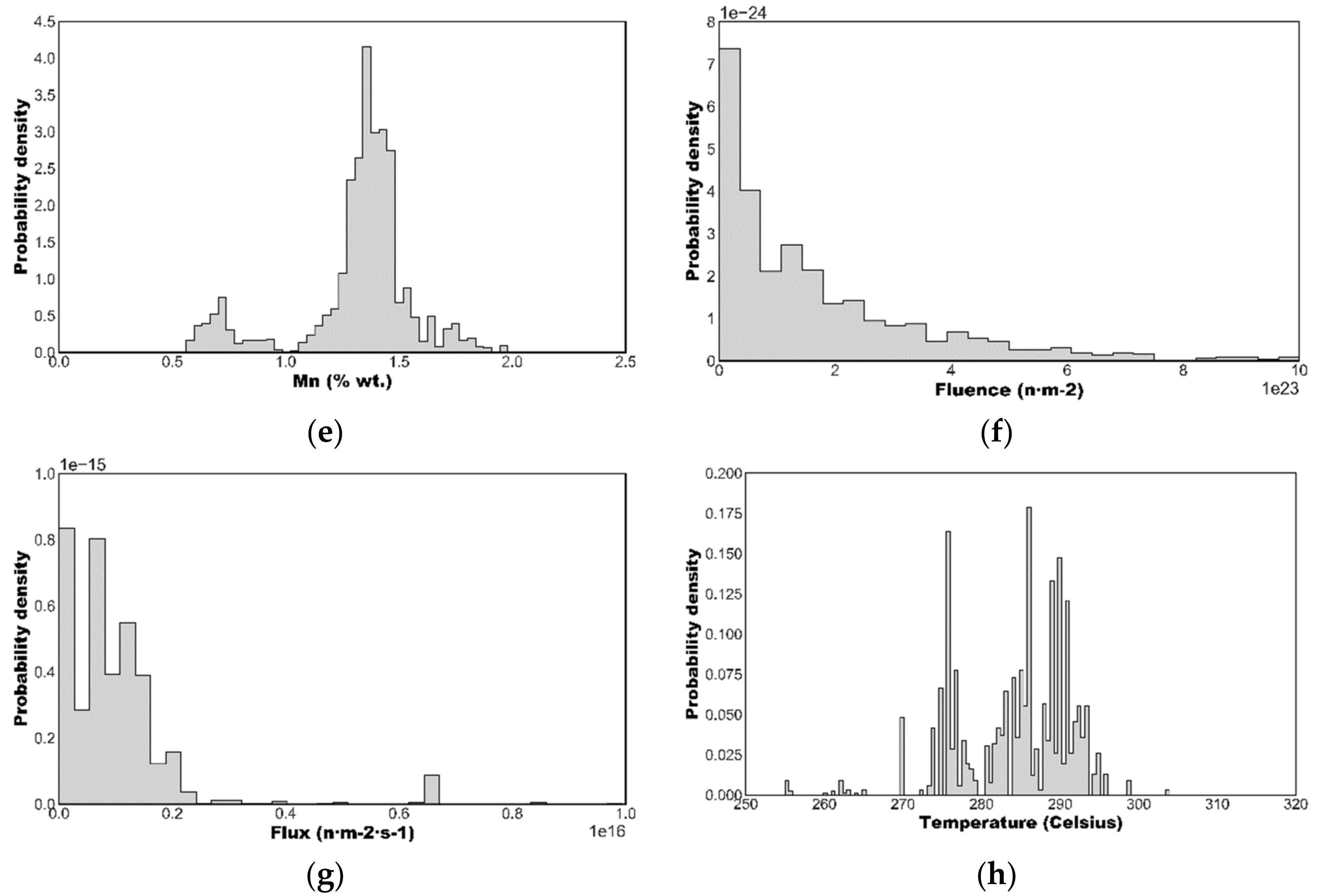
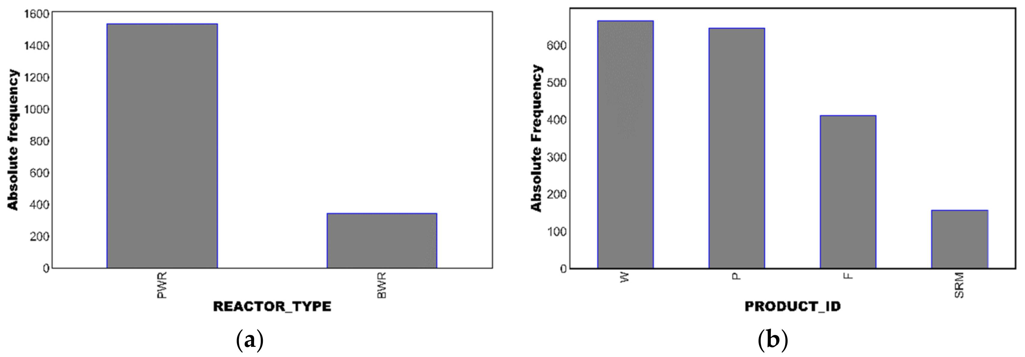
2.1. The ASTM PLOTTER Database
- The TTS is the target (or variable to be predicted).
- The predictor (or regressor) variable includes numeric vales to describe the chemical composition (Cu, Ni, P, Mn) and irradiation conditions (neutron fluence, flux and temperature) and also indicator/categorical variables describing the product type (welds, plates, forgings, or SRM plates) and the reactor type (BWR or PWR).
2.2. The ASTM E900-15 Embrittlement Trend Curve
2.3. Machine Learning
2.3.1. Scope of the Analysis
2.3.2. Data Preprocessing
- Data outliers can result in longer training times and less accurate models. Outliers, which were defined as data points beyond a z-score (see Formula (8) for the definition of the z-score of the observation xi, where mx is the sample mean and sx is the sample standard deviation) |z| > 3.0, were not observed in the PLOTTER BASELINE dataset.
- Multicollinearity is potentially harmful for the performance of the model; it may reduce its statistical significance and make it difficult to determine the importance of a feature to the target variable. The Pearson’s correlation matrix (see Expression (9) for the definition of the sample Pearson correlation coefficient, r) of the dataset, Figure 3, was estimated to identify correlations between features. It was decided to remove one of the features of every couple with a correlation coefficient exceeding (in absolute value) 0.60. Nevertheless, since the maximum correlations observed were between Cu and P (r = 0.48), no features were eliminated.
- Standardization/feature scaling of a dataset is mandatory for some ML algorithms and advisable for others. In this study, features were scaled through the StandardScaler provided by Scikit-Learn [13] which standardizes the features by removing the mean and scaling to unit variance.
- Nominal categorical variables (reactor type and product id) were subjected to the Scikit-Learn OneHotEncoder [13].
2.3.3. ML Algorithms
- In MLR, the relationship between the predictors and the response variable is fitted through a multilinear equation to the observed data. MLR is considered as a baseline algorithm for regression, i.e., a simple model with a reasonable chance of providing decent results. Baseline models are easy to deploy and provide a benchmark to evaluate the performance of more complex models. Many early approaches to embrittlement modeling for RPV steels adopted a “chemistry factor” that was a weighted sum of the contributions of different chemical elements to embrittlement [16]. The data fittings needed to establish these chemistry factors were essentially multi-linear regressions.
- In KNN, regression is carried out for a new observation by averaging the target variable of the ‘K’ closest observations (the neighbors) with weights that can be uniform or proportional to the inverse of the distance from the query point. KNN is an example of an instance-based algorithm that depends on the memorization of the dataset; then, predictions are obtained by looking into these memorized examples. The distance between instances is based on features (e.g., Cu, Ni, temperature) important to the target variable (TTS) and is quantified through the Minkowski metric, which depends on the power parameter, ‘p’. When p = 1, this is equivalent to using the Manhattan distance and for p = 2, the Euclidean distance.
- CARTs were introduced in 1984 by Breiman et al. [17]. These “trees” may be thought of as flowcharts; they have a branching structure in which a series of decisions is used to make a prediction that either classifies the data (outputting a categorical value) or regresses the data (outputting a continuous value). The CART splits the dataset to form a tree structure; the branching decisions (called decision nodes) are guided by the homogeneity of data. The resultant tree has “leaf nodes” at the end of the branches. Ideally, each leaf represents a more-or-less uniform response of the target variable, be it categorical or continuous. The Gini index and the entropy are the most common scores to measure the homogeneity of the data and to decide which feature should be selected for the next split. Building a decision tree requires finding the attribute that returns the highest information gain (which is defined as the entropy of the parent node minus the entropy of the child nodes after the dataset has been split on that attribute) or the highest reduction in the Gini index. The main advantages of decision trees are that the interpretation of results is straightforward and that they implicitly perform a feature selection since the earliest (or top) nodes of the tree are the most important variables within the dataset. The main limitation of a CART is that when a decision tree grows and becomes very complex, it usually displays a high variance and a low bias, which are evidence of overfitting. This makes it difficult for the model to generalize and to incorporate new data.
- The support vector machine (SVM) algorithm was originally designed as a classifier [18] but may also be used for regression, SVR, and feature selection [19]. In classification, SVM determines the optimal separating hyperplane between linearly separable classes maximizing the margin, which is defined as the distance between the hyperplane and the closest points on both sides (the support vectors). For non-perfectly separable classes, SVM must be modified to allow some points to be misclassified, which is achieved by introducing a “soft margin” [20]. Datasets that are highly nonlinear may in some cases be (linearly) separated after being (nonlinearly) mapped into a higher dimensional space [21]. This mapping gives rise to the kernel, which can be chosen by the user among different options such as linear, sigmoid, Gaussian or polynomial. The appropriate kernel function is selected by trial and error on the test set. In this case, SVM is referred to as kernelized SVM.
- Ensemble learning is a paradigm that focuses on training a large number of low-accuracy models, which are called “weak learners,” and combining their predictions to obtain a high accuracy meta-model. Decision trees (as just described under CARTs) are the most widely used weak learners. The idea behind ensemble learning is that if the trees are not identical and they predict the target variable with an accuracy that is slightly better than random guessing, a prediction based on some sort of weighted voting of a large number of such trees will improve accuracy. Ensemble methods are classified into bagging-based and boosting-based, which are designed to reduce variance and bias, respectively.
- ○
- Bagging (which stands for bootstrap aggregation) is the application of the bootstrap procedure (i.e., random sampling with replacement) to a high-variance ML model (e.g., a regression tree). Many models are created, and every model is trained in parallel. Each of the models is trained on a subset of the whole dataset composed of a number of observations randomly selected with replacement using a subset of features. The predicted value produced by bagging is simply the average of the predictions from all the models. The most widely used bagging-based ML algorithm is RF [22], which uses shallow classification trees as the weak learners. The most important hyperparameters to tune in a RF are the number of trees and the size of the random subset of the features to consider at each split. By using multiple samples of the original dataset, the variance of the ensemble RF model is reduced, as is the overfitting (see Section 2.3.4).
- ○
- Boosting consists of using the original training data and iteratively creating multiple models by using a weak learner, usually a regression tree. Each new model tries to fix the errors made by previous models. Unlike bagging, which aims at reducing variance, boosting is mainly focused on reducing bias. In adaptative boosting, AB, and in GB, the ensemble model is defined as a weighted sum of weak learners. The weights are placed more heavily on the data that were poorly predicted by the initial weak learners, thereby gradually improving the accuracy of the overall model. XGB is an algorithm that uses a GB framework developed in 2016 by Chen and Guestrin [23]. Among its advantages, it provides a good combination of performance and processing time through systems optimization and algorithmic enhancements (such as parallelized implementation).
- ANNs are used for data classification, regression and pattern recognition. A basic ANN contains a large number of neurons arranged in layers. An MLP begins with an input layer, which contains one or more hidden layers that are trained to make decisions, and an output layer. The nodes of consecutive layers are connected, and these connections have weights associated with them. During training, weights are initially assigned randomly. Known data are then fed forward through the network from the input nodes, through the hidden nodes (if any), and to the output nodes. The output of every neuron is obtained by applying an activation function to the linear combination of inputs (weights) to the neuron; sigmoid, tanh and rectified linear unit (ReLu) are the most widely used activation functions. MLPs are trained to produce better answers through backpropagation. During backpropagation, the network is provided with feedback concerning outputs that have been incorrectly predicted. The network then changes the weights associated with the nodes in the hidden layers to produce a more accurate output. Gradient descent, Newton, conjugate gradient and Levenberg–Marquardt are different algorithms used to train an ANN.
2.3.4. Evaluation of Machine Learning Algorithms
3. Results
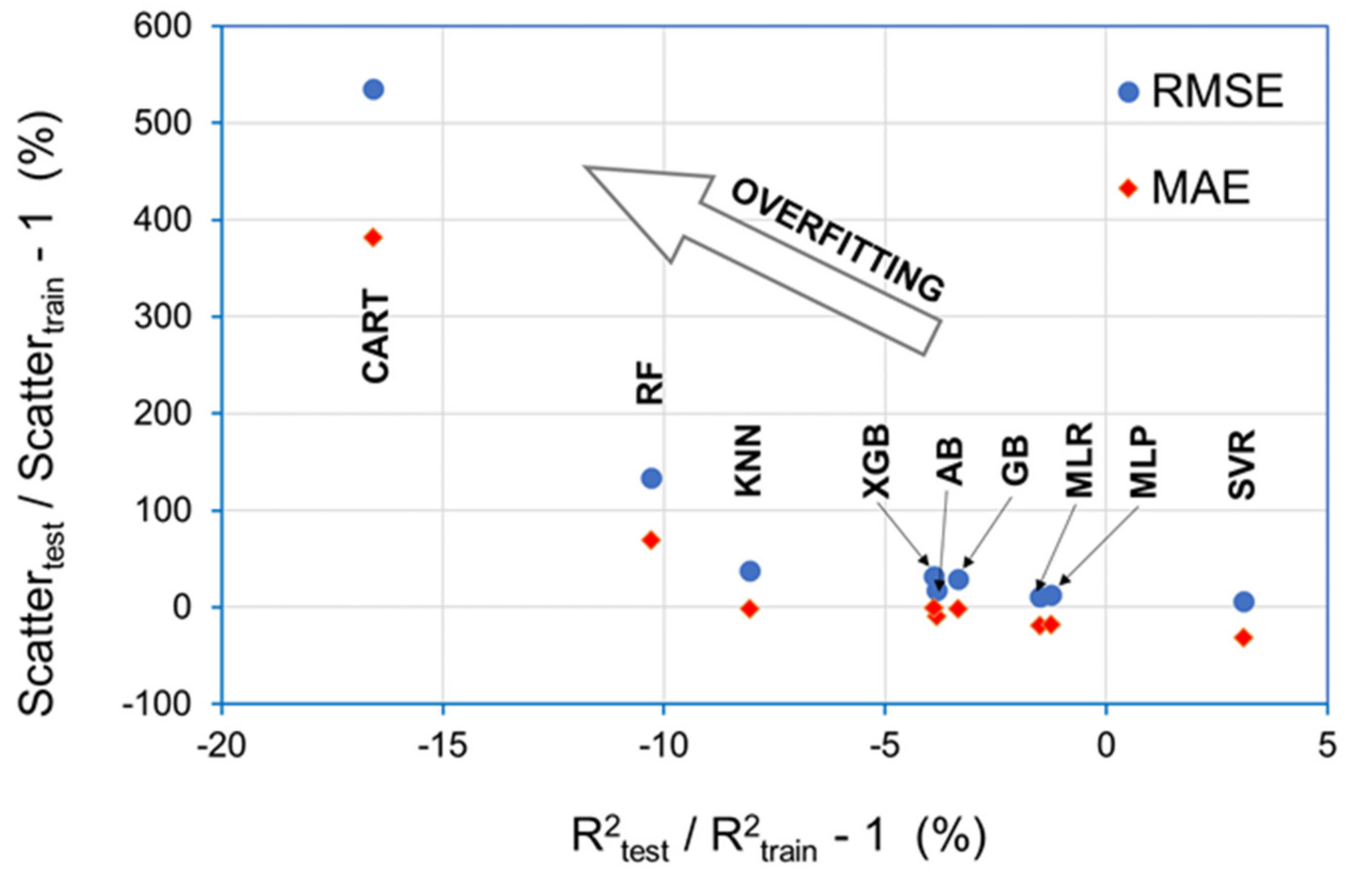
3.1. Selection of the Optimum Algorithm
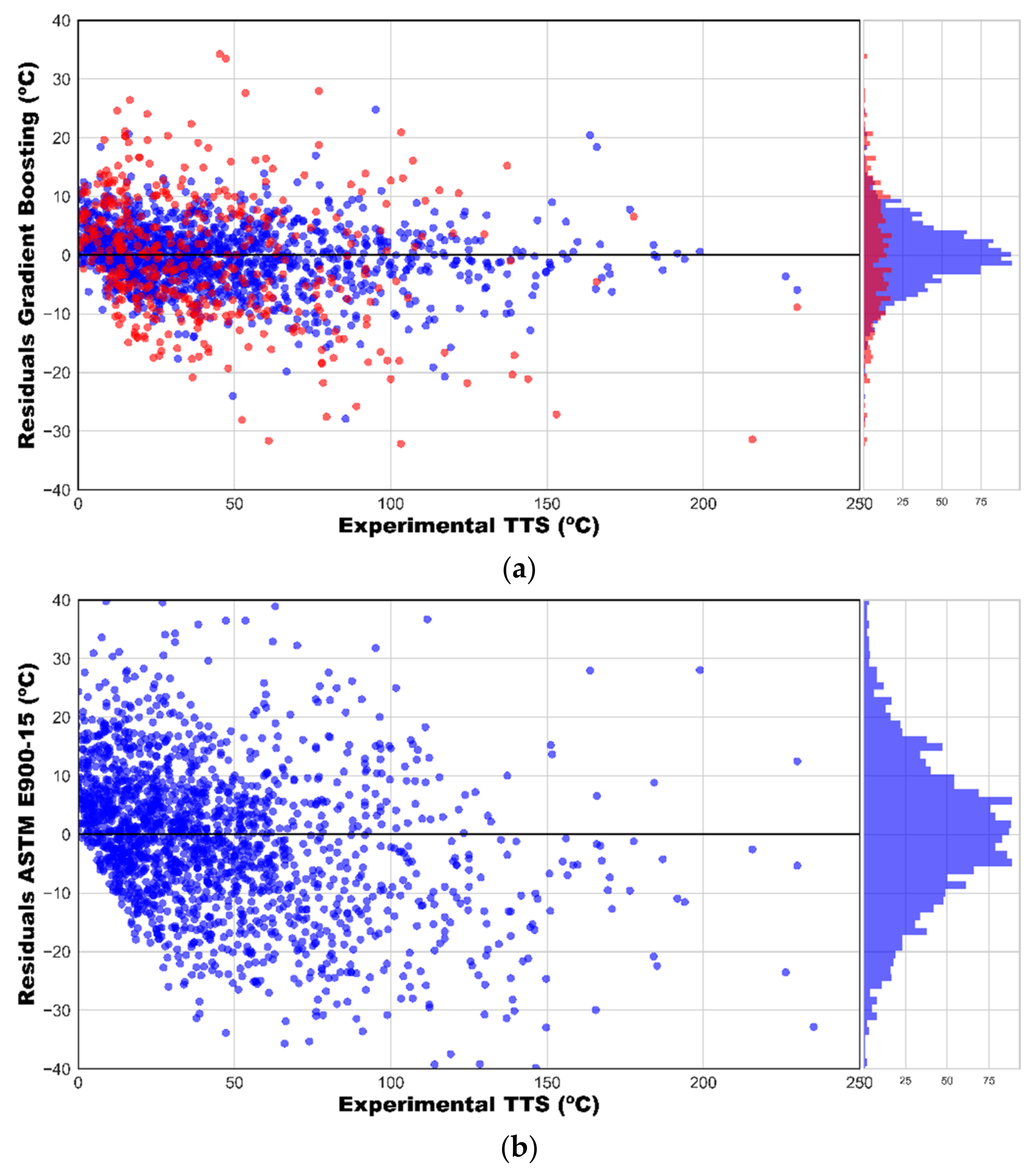
3.2. Regression with Gradient Boosting
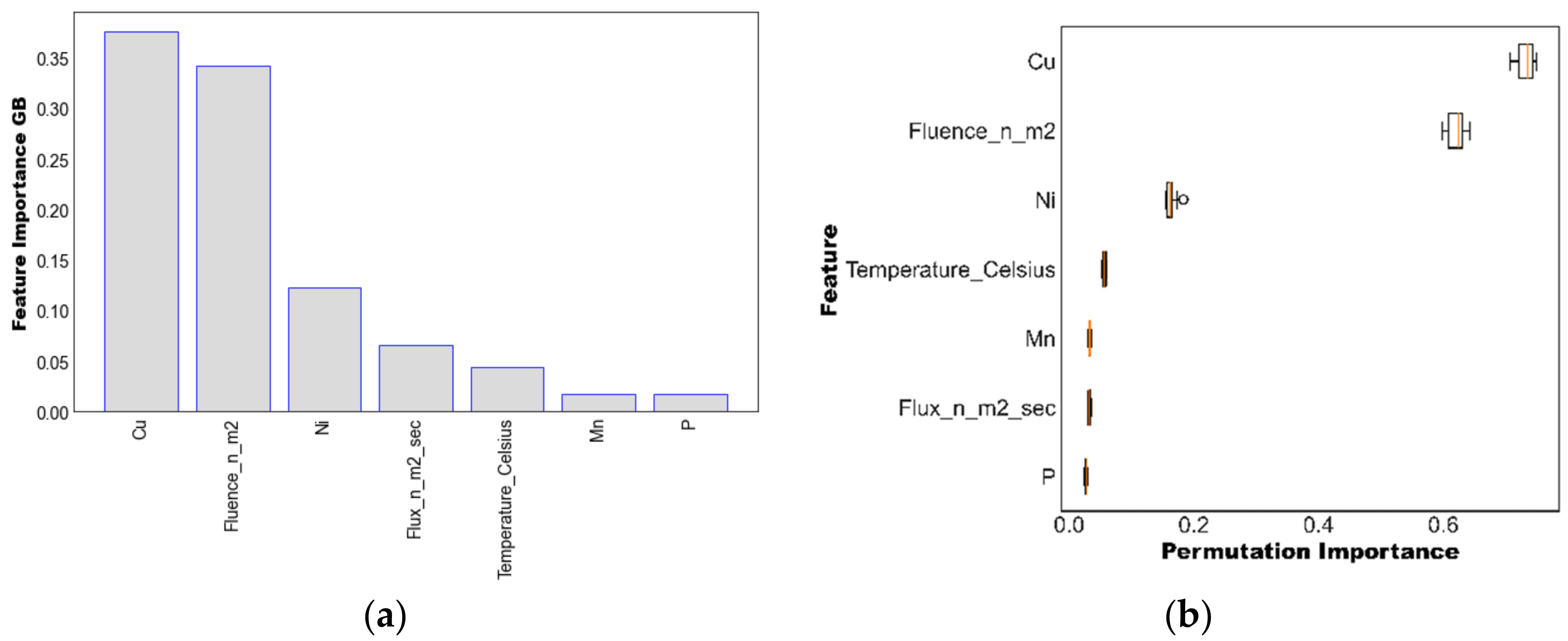
3.3. Assessment of Importance of the Features
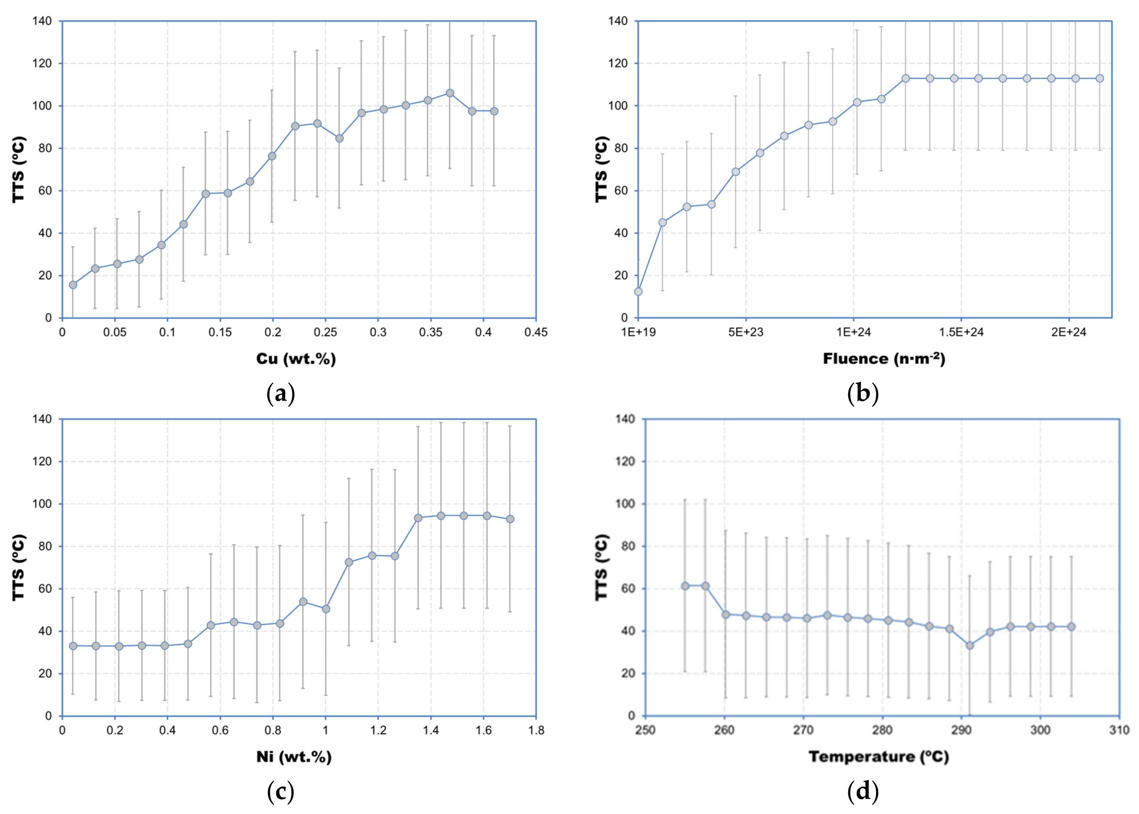
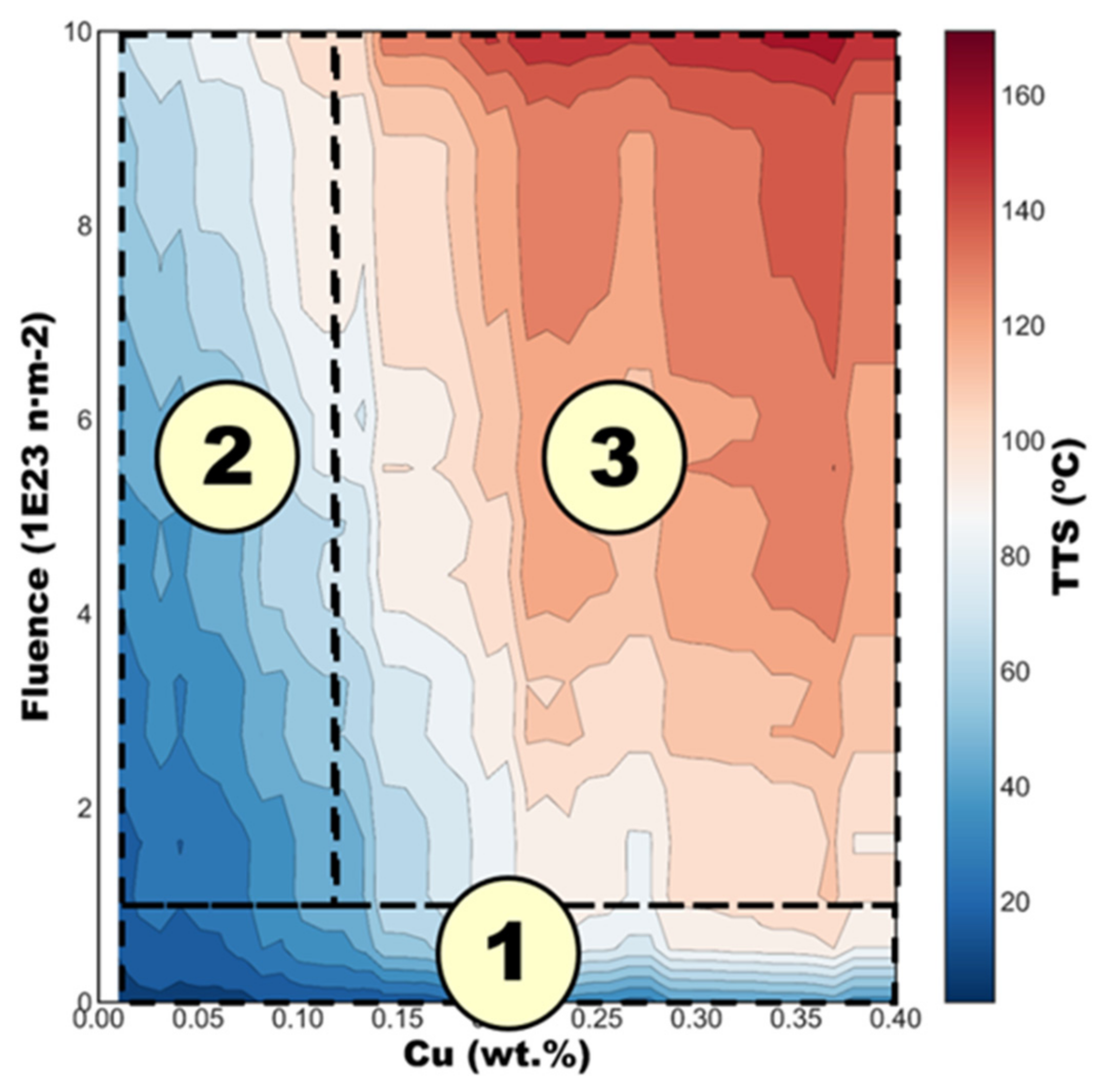
3.4. Individual Conditional Expectation Plots and Interaction Plots
4. Discussion
5. Conclusions
- Best results in the test set were provided by the GB algorithm, which provided a value of R2 = 0.91 and a root mean squared error ≈10.5 °C for the test dataset. These results outperformed the prediction ability of existing trend curves, including ASTM E900-15, reducing the prediction uncertainty by ≈20%.
- The impurity-based and the permutation-based feature importances obtained from the optimized GB model suggest that copper, fluence, and temperature are the most important features in estimating TTS, while features such as phosphorus and manganese play minor roles, in accordance with existing atomistic, physical and empirical models on neutron embrittlement.
- Noticeable interactions between Cu-fluence, Cu-Ni and fluence-Ni were observed
- The individual conditional expectation (ICE) plot for Cu yielded a classification of low Cu and high Cu consistent with the regression model of the ASTM E900-15.
Author Contributions
Funding
Institutional Review Board Statement
Informed Consent Statement
Data Availability Statement
Conflicts of Interest
Abbreviations
| ΔYS | Yield strength increase |
| AB | AdaBoost |
| ANN | Artificial neural networks |
| BWR | Boiling water reactor |
| CART | Classification and regression tree |
| ETC | Embrittlement trend curve |
| GB | Gradient boosting |
| ICE | Individual conditional expectation |
| KNN | K-nearest neighbors |
| LTO | Long-term operation |
| LWR | Light water reactor |
| MAE | Mean absolute error |
| ML | Machine learning |
| MLP | Multi-layer perceptron |
| MLR | Multiple linear regression |
| MTR | Material test reactor |
| NRMSE | Normalized root mean square error |
| PWR | Pressurized water reactor |
| r | Sample Pearson correlation coefficient |
| R2 | Coefficient of determination |
| ReLu | Rectified linear unit |
| RF | Random forest |
| RMSE | Root mean square error |
| RPV | Reactor pressure vessel |
| SVR | Support vector regression |
| TTS | Transition temperature shift |
| XGB | Extreme gradient boosting |
| VVER | Water-water energetic reactor |
| z | z-score |
References
- Eason, E.D.; Wright, J.E.; Odette, G.R. Improved Embrittlement Correlations for Reactor Pressure Vessel Steels; Division of Engineering Technology, Office of Nuclear Regulatory Research, US Nuclear Regulatory Commission: Washington, DC, USA, 1998. [Google Scholar]
- Regulatory Guide 1.99 (Revision 2): Radiation Embrittlement of Reactor Vessel Materials; USNRC: Washington, DC, USA, 1998.
- Eason, E.D.; Odette, G.R.; Nanstad, R.K.; Yamamoto, T. A Physically Based Correlation of Irradiation-Induced Transition Temperature Shifts for RPV Steels; U.S. Nuclear Regulatory Commission: Oak Ridge, TN, USA, 2007. [Google Scholar]
- ASTM E900-15e2, Standard Guide for Predicting Radiation-Induced Transition Temperature Shift in Reactor Vessel Materials; ASTM International: West Conshohocken, PA, USA, 2015.
- Hashimoto, Y.; Nomoto, A.; Kirk, M.; Nishida, K. Development of new embrittlement trend curve based on Japanese surveillance and atom probe tomography data. J. Nucl. Mater. 2021, 553, 153007. [Google Scholar] [CrossRef]
- The Fourth Paradigm: Data-Intensive Scientific Discovery; Hey, T.; Tansley, S.; Tolle, K. (Eds.) Microsoft Research: Washington, DC, USA, 2009. [Google Scholar]
- Unger, J.F.; Könke, C. Neural networks as material models within a multiscale approach. Comput. Struct. 2009, 87, 1177–1186. [Google Scholar] [CrossRef]
- Zopf, C.; Kaliske, M. Numerical characterisation of uncured elastomers by a neural network based approach. Comput. Struct. 2017, 182, 504–525. [Google Scholar] [CrossRef]
- Kalidindi, S.R.; Niezgoda, S.R.; Salem, A.A. Microstructure informatics using higher-order statistics and efficient data-mining protocols. J. Miner. 2011, 63, 34–41. [Google Scholar] [CrossRef]
- Rajan, K. Materials informatics. Mater. Today 2005, 8, 38–45. [Google Scholar] [CrossRef]
- Guido, S.; Müller, A. Introduction to Machine Learning with Python: A Guide for Data Scientists; O’Reilly Media: Newton, MA, USA, 2016; ISBN 978-1449369415. [Google Scholar]
- Geron, A. Hands-On Machine Learning with Scikit-Learn and TensorFlow; O’Reilly Media, Inc.: Newton, MA, USA, 2017; ISBN 978-1491962299. [Google Scholar]
- Pedregosa, F.; Varoquaux, G.; Gramfort, A.; Michel, V.; Thirion, B.; Grisel, O.; Blondel, M. Scikit-learn. J. Mach. Learn. Res. 2011, 12, 2825–2830. [Google Scholar]
- Wolpert, D.H. The Supervised Learning No-Free-Lunch Theorems. In Proceedings of the 6th Online World Conference on Soft Computing in Industrial Applications, On the Internet (World Wide Web), 10–24 September 2001; Springer: Berlin/Heidelberg, Germany, 2001; pp. 1–20. [Google Scholar]
- Wolpert, D.H.; Macready, W.G. No free lunch theorems. IEEE Trans. Evol. Comput. 1997, 1, 67–82. [Google Scholar] [CrossRef] [Green Version]
- Regulatory Guide 1.99 (Revision 0): Effects of Residual Elements on Predicted Radiation Damage to Reactor Vessel Materials; USNRC: Washington, DC, USA, 1975.
- Breiman, L.; Friedman, J.; Stone, C.J.; Olshen, R.A. Classification and Regression Trees; Chapman and Hall/CRC: London, UK, 1984; ISBN 978-0412048418. [Google Scholar]
- Vapnik, V.; Chervonenkis, A. A note on one class of perceptrons. Autom. Remote Control 1964, 25, 61–68. [Google Scholar]
- Cao, F.L.; Bai, H.B.; Yang, J.C.; Ren, G.Q. Analysis on Fatigue Damage of Metal Rubber Vibration Isolator. Adv. Mater. Res. 2012, 490–495, 162–165. [Google Scholar] [CrossRef]
- Mohamed, A.E. Comparative Study of Supervised Machine Learning Techniques for Intrusion Detection. In Proceedings of the Fifth Annual Conference on Communication Networks and Services Research (CNSR’07), Frederlcton, NB, Canda, 14–17 May 2007; Volume 14, pp. 5–10. [Google Scholar] [CrossRef]
- Boser, B.E.; Guyon, I.M.; Vapnik, V.N. A training algorithm for optimal margin classifiers. In Proceedings of the Fifth Annual Workshop on Computational Learning Theory, Pittsburgh, PA, USA, 27–29 July 1992; pp. 144–152. [Google Scholar] [CrossRef]
- Breiman, L. Random forests. Mach. Learn. 2001, 45, 5–32. [Google Scholar] [CrossRef] [Green Version]
- Chen, T.; Guestrin, C. XGBoost: A scalable tree boosting system. In Proceedings of the ACM SIGKDD International Conference on Knowledge Discovery and Data Mining, San Francisco, CA, USA, 13–17 August 2016; pp. 785–794. [Google Scholar]
- Goldstein, A.; Kapelner, A.; Bleich, J.; Pitkin, E. Peeking Inside the Black Box: Visualizing Statistical Learning with Plots of Individual Conditional Expectation. J. Comput. Graph. Stat. 2015, 24, 44–65. [Google Scholar] [CrossRef]
- Chollet, F. Deep Learning with Python; Manning Publications: New York, NY, USA, 2018; ISBN 978-1617294433. [Google Scholar]
- Soneda, N.; Dohi, K.; Nomoto, A.; Nishida, K.; Ishino, S. Embrittlement Correlation Method for the Japanese Reactor Pressure Vessel Materials. In Effects of Radiation on Nuclear Materials and the Nuclear Fuel Cycle: 24th Volume; Busby, J., Hanson, B., Eds.; ASTM International: West Conshohocken, PA, USA, 2010; pp. 64–93. ISBN 978-0-8031-8417-6. [Google Scholar]
- Lee, G.-G.; Kim, M.-C.; Lee, B.-S. Machine learning modeling of irradiation embrittlement in low alloy steel of nuclear power plants. Nucl. Eng. Technol. 2021, 53, 4022–4032. [Google Scholar] [CrossRef]
- Kirk, M. A wide-range embrittlement trend curve for western reactor pressure vessel steels. ASTM Spec. Tech. Publ. 2013, 1547, 20–51. [Google Scholar] [CrossRef]
- U.S. NRC. Adjunct for ASTM E900-15: Technical Basis for the Equation used to Predict Radiation-Induced Transition Temperature Shift in Reactor Vessel Materials; U.S. NRC: Washington, DC, USA, 2015. [Google Scholar]
- Ferreño, D.; Sainz-Aja, J.A.; Carrascal, I.A.; Cuartas, M.; Pombo, J.; Casado, J.A.; Diego, S. Prediction of mechanical properties of rail pads under in-service conditions through machine learning algorithms. Adv. Eng. Softw. 2021, 151, 102927. [Google Scholar] [CrossRef]
- Todeschini, P.; Kirk, M. Further assessment of the ASTM E900-15 transition temperature shift relationship. In Proceedings of the IGRDM-19: 19th Meeting of the International Group on Radiation Damage Mechanisms in Pressure Vessel Steels, Asheville, NC, USA, 10–15 April 2016. [Google Scholar]
- Kirk, M.; Hashimoto, Y.; Nomoto, A.; Yamamoto, M.; Soneda, N. Application of a Machine Learning Approach Based on Nearest Neighbors to Extract Embrittlement Trends from RPV Surveillance Data. In Proceedings of the 2021 Meeting of the International Group on Radiation Damage, Mol, Belgium, 8–10 September 2021. [Google Scholar]


| Train Dataset | Test Dataset | |||||
|---|---|---|---|---|---|---|
| Regressor | R2 | RMSE (°C) | MAE (°C) | R2 | RMSE (°C) | MAE (°C) |
| MLR | 0.736 | 18.87 | 18.87 | 0.725 | 20.91 | 15.34 |
| KNN | 0.881 | 12.66 | 12.66 | 0.810 | 17.39 | 12.51 |
| CART | 0.995 | 2.59 | 2.58 | 0.830 | 16.44 | 12.44 |
| SVR | 0.579 | 23.85 | 23.85 | 0.597 | 25.32 | 16.45 |
| RF | 0.972 | 6.10 | 6.10 | 0.872 | 14.26 | 10.34 |
| AB | 0.810 | 16.01 | 16.01 | 0.779 | 18.77 | 14.50 |
| GB | 0.927 | 9.94 | 9.94 | 0.896 | 12.87 | 9.81 |
| XGB | 0.924 | 10.10 | 10.10 | 0.888 | 13.36 | 10.06 |
| MLP | 0.874 | 13.03 | 13.03 | 0.863 | 14.76 | 10.76 |
| Regressor | Hyperparameters |
|---|---|
| MLR | N/A |
| KNN | n_neighbors = 5, weights = ‘uniform’, algorithm = ‘auto’, leaf_size = 30, p = 2, metric = ‘minkowski’ |
| CART | criterion = ‘squared_error’, splitter = ‘best’, min_samples_split = 2, min_samples_leaf = 1 |
| SVR | kernel = ‘rbf’, degree = 3, gamma = ‘scale’, tol = 0.001, C = 1.0, epsilon = 0.1, shrinking = True, cache_size = 200, verbose = False, max_iter = −1 |
| RF | n_estimators = 100, criterion = ‘squared_error’, min_samples_split = 2, min_samples_leaf = 1, max_features = ‘auto’, bootstrap = True, oob_score = False, verbose = 0, warm_start = False |
| AB | n_estimators = 50, learning_rate = 1.0, loss = ‘linear’ |
| GB | oss = ‘squared_error’, learning_rate = 0.1, n_estimators = 100, subsample = 1.0, criterion = ‘friedman_mse’, min_samples_split = 2, min_samples_leaf = 1, max_depth = 3, alpha = 0.9, warm_start = False, validation_fraction = 0.1, tol = 0.0001 |
| XGB | ‘objective’: ‘reg:squarederror’, ‘importance_type’: ‘gain’, ‘n_estimators’: 100 |
| MLP | hidden_layer_sizes = (100), activation = ‘relu’, solver = ‘adam’, alpha = 0.0001, batch_size = ‘auto’, learning_rate = ‘constant’, learning_rate_init = 0.001, power_t = 0.5, max_iter = 200, shuffle = True, tol = 0.0001, verbose = False, momentum = 0.9, nesterovs_momentum = True, early_stopping = False, validation_fraction = 0.1, beta_1 = 0.9, beta_2 = 0.999, epsilon = 1 × 10⁻⁸, n_iter_no_change = 10, max_fun = 15,000 |
| Train | Test | Train + Test | ASTM E900-15 | |
|---|---|---|---|---|
| R2 | 0.977 | 0.914 | 0.963 | 0.875 |
| RMSE (°C) | 5.73 | 10.54 | 7.24 | 13.32 |
| NRMSE | 0.159 | 0.277 | 0.198 | 0.364 |
| MAE (°C) | 4.23 | 8.37 | 5.26 | 10.12 |
Publisher’s Note: MDPI stays neutral with regard to jurisdictional claims in published maps and institutional affiliations. |
© 2022 by the authors. Licensee MDPI, Basel, Switzerland. This article is an open access article distributed under the terms and conditions of the Creative Commons Attribution (CC BY) license (https://creativecommons.org/licenses/by/4.0/).
Share and Cite
Ferreño, D.; Serrano, M.; Kirk, M.; Sainz-Aja, J.A. Prediction of the Transition-Temperature Shift Using Machine Learning Algorithms and the Plotter Database. Metals 2022, 12, 186. https://doi.org/10.3390/met12020186
Ferreño D, Serrano M, Kirk M, Sainz-Aja JA. Prediction of the Transition-Temperature Shift Using Machine Learning Algorithms and the Plotter Database. Metals. 2022; 12(2):186. https://doi.org/10.3390/met12020186
Chicago/Turabian StyleFerreño, Diego, Marta Serrano, Mark Kirk, and José A. Sainz-Aja. 2022. "Prediction of the Transition-Temperature Shift Using Machine Learning Algorithms and the Plotter Database" Metals 12, no. 2: 186. https://doi.org/10.3390/met12020186
APA StyleFerreño, D., Serrano, M., Kirk, M., & Sainz-Aja, J. A. (2022). Prediction of the Transition-Temperature Shift Using Machine Learning Algorithms and the Plotter Database. Metals, 12(2), 186. https://doi.org/10.3390/met12020186