Abstract
Stress analysis and deformation prediction have always been the focuses of the field of mechanics. The accurate force prediction in plate deformation plays important role in the production, processing and performance analysis of materials. In this paper, we propose an ARIMA-FEM method, which can be used to solve some mechanical problems of 2D porous elastic plate. We have given a detailed theory and solving steps of ARIMA-FEM. In addition, three numerical examples are given to predict the stress–strain of thin porous elastic metal plates. This article uses CST, LST and Q4 elements to discrete the rectangular plates, square plates and circle plates with holes. As for variable force prediction, this paper compared with linear regression, nonlinear regression and neural network prediction, and the results show that the ARIMA method has a higher prediction accuracy. Furthermore, we calculate the numerical solution at four mesh scales, and the numerical convergence is consistent with the theoretical convergence, which also shows the effectiveness of our method. The image smoothing algorithm is applied to keep edge information with high resolution, which can more concisely describe the plate internal changes. Finally, the application scope of ARIMA-FEM, model expansion, superconvergence analysis and other issues have been given enlightening views in the discussion section. In fact, this algorithm combined statistics and mechanics. It also reflects the knowledge integration of interdisciplinary and uses it better to serve practical applications.
1. Introduction
1.1. Research Motivation and Significance
The problem of material deformation and stress analysis has always been the focus of research in the field of material application and computational mechanics. For the problem of solid deformation analysis, it has gradually transited from single classical mechanics to multidisciplinary intersection. In addition, there are also many practical application backgrounds regarding mechanical prediction of poroelastic plate in real life and engineering applications. For example, sheet metal parts processed by machine tools, the impact of aircraft engine vibration on the performance of wing materials, indoor metal plate decoration materials, metal plate welding and precision cutting and so on. However, there are still many defects in the mechanical application of thin plates, which need to be improved urgently. The traditional finite element method has hysteresis and can not test the mechanical properties of metal thin plates in advance. At present, the accuracy and convergence of predicting the mechanical changes of thin plates are still in a state to be studied. The main purpose of this paper is to predict the stress problem of thin plate, improve the prediction accuracy, provide the numerical convergence analysis and output the cloud map of stress, strain and displacement. The significance of our research is that researchers quickly compare the stress changes of thin plates at a certain time in the future to improve the accuracy of numerical solutions.
1.2. Related Work
Porous metals have many applications in daily life and industry, such as filtration, sound absorber [1,2], thermal energy storage [3], electrochemical isolation equipment or biomedical materials [4]. Meanwhile, powder metallurgy techniques are the preferred method of manufacturing porous metals [5]. Porous metal materials have good functions of filtration, separation and purification. Porous metal membrane can realize seawater desalination and purification. This green filtration technology has the advantages of high flux, simple operation and high temperature resistance [6]. In addition, porous metal combustion vessel has the function of filtration and can extract rare metals from various combustible materials (such as coal and petroleum waste) [7]. The results show that the rare metal extraction method is very effective for combustible media with low initial metal concentration.
It can be seen that the research and design of material structure are inseparable from the analysis of mechanical properties. The accurate the mechanical model is helpful for the application of materials in different conditions. The common mechanical tests of plate materials include tensile, torsion, compression [8] and penetrating plate [9]. There are also many numerical methods that can be used to simulate this problem. The element vertex finite volume method (CV-FVM) is used to analyze the porous structure of the thermoelastic material, and then using the staggered mesh to discretize the control equation, and the nonlinear heat conduction equation is solved a convergent temperature solution. The distribution of thermal stress is more sensitive than temperature and deformation, and the existence of pores helps reduce thermal stress to a certain extent [10]. Nonlinear finite element method (FEM) combined with artificial neural network (ANN) is used to solve the crack strength of elastic plate. Compared with thick plate, pitting corrosion has less effect on the reduction of ultimate strength [11]. Moreover, combining smoothed-particle hydrodynamics (SPH) and the finite element method (FEM) is developed to predict the waves propagating in the thin elastic plate [12]. It is shown that the mathematical solution effectively explains the characteristics of the nonlinear waves in the elastic plate.
Porous plates often be effected by external force load in the application, which can be concentrated force, surface force, volume force and so on.The characterization of mechanical experiments usually requires higher experimental cost, but numerical simulation has the characteristics of fast speed and low cost. In fact, there are many methods for force prediction, external forces with different trends have different prediction methods. Accurate prediction of the cutting force is the key factor in cutting simulation and optimization [13,14]. Three-dimensional cutting force and turning force prediction have very important application value, which is based on hybrid finite element and predictive machining theory [15]. In order to to predict the thermal deformation of the rotor of the rotary air preheater, a new soft sensor DBN-IPSO-SVR was proposed [16]. The new prediction method combines three traditional methods, namely the deep belief network (DBN) [17], improved particle swarm optimization (IPSO) [18] and support vector regression (SVR) [19]. The experimental results show that the model has high prediction accuracy.
Among the existing theories, there are relatively few models for predicting the force analysis of porous plates with high precision. When the change trend of external force is relatively large, it is difficult to ensure high accuracy by ordinary prediction methods. Machine learning methods rely on more data, and the optimal model parameters need to be tried and adjusted many times. BP neural network prediction can also be used to predict simple forces with changing trends. Such as, predicting the quality of the injected plastic parts based on key process variables. The method has lower time required for optimizing of process conditions [20]. In addtion, during the process of 3D curved hull plate forming, springback will cause serious influence on the forming accuracy, it is necessary to solve the problem of springback in the hull plate forming process by establishing a nonlinear model of plate and springback based on BP neural network [21]. Artificial neural networks (ANN) is not only an computationally efficient analysis tool, but also can predict the buckling load of laminated composite stiffened panels subjected to in-plane shear loading [22]. The results shows that the trained neural network will be very useful in optimization applications and have a good predicted the shear buckling load.
The mechanical performance analysis of perforated plates is also suitable for several common plate models. For example, a new weak Galerkin finite element method is analyzed for the Reissner–Mindlin plate model, this method achieves uniform convergence with respect to plate thickness (the so-called locking-free) without any projection, reduced integration [23]. In reference [24], the obstacle problem in Kirchhoff–Love plate model is simulated by variational inequality. Under the assumption of the regularity of the solution, the optimal order error estimation under the discrete energy norm is derived. In addition, the mechanical prediction problem also includes crack growth. For aircraft fatigue life prediction and crack growth modeling, the simulation results predict the contact force and shear deformation [25]. The most common method for locating public facilities is the micro-tunnel model, but prediction of the total jacking force is very complex. a probabilistic observational approach are proposed, which can be used to predict the jacking force of the micro-tunnel belongs to the prediction within the framework of probability. The error depends on the proper degree of the probability model [26,27]. The results show that this method is very useful for the monitored field data and highlights a significant.
In this paper, an autoregressive integrated moving average (ARIMA) based model red which combines both statistical and mechanical knowledge, are developed to predict the variable force. ARIMA model is a kind nonstationary prediction model composed by AR and MA models, which was systematically proposed by Box and Jenkins in Ref. [28]. The data generated by predicting the change over time are often called a random sequence, and a suitable mathematical model can be established to estimate future data based on historical data values. The parameter of the ARIMA model could be obtained by maximum likelihood estimation or least squares estimation. This algorithm has been widely used in finance, commercial sale prediction and engineering [29,30,31], it has achieved a good prediction results. However, it is very rare to introduce this method into the prediction of deformation change in mechanical problems, which also highlights the importance of our work.
1.3. Contributions
The main purpose of this paper is to predict the change of mechanical properties of porous elastic plates. ARIMA-FEM method could help to obtain the variation of internal structure of materials, so as to evaluate and predict the practical physical application problems and improve the application scope of materials. The contribution of this paper is divided into four aspects. Firstly, the ARIMA-FEM method is proposed, which combines the ARIMA prediction model with the FEM numerical solution of the 2D linear elastic equation. This method can predict the stress, strain, displacement and other physical quantities in the porous elastic metal plate in a certain period in the future. The second contribution is the comparison of several numerical prediction methods including linear regression, nonlinear regression and BP neural network prediction. The numerical results show that ARIMA prediction results are relatively good for time series with large fluctuation trend. The third contribution is to verify the consistency between numerical convergence and theoretical convergence, and also to test the effectiveness of the proposed method. The fourth contribution is to use high resolution smoothing method to enhance the visualization effect of stress, strain and displacement in cloud images, and ensure the pixel value near the image edge. The change of edge information is also the focus of mechanical attention.
1.4. Structure and Framework of This Paper
This paper consists of five sections, the focus of each parts will be briefly summarized. Section 2 mainly introduces the ARIMA-FEM theories and the solving steps, as well as including the theory of CST, LST and Q4 elements for solving linear elastic problems. Meanwhile, we provide the detailed forms of stress boundary conditions and displacement boundary conditions. Section 3 is mainly about convergence analysis and error estimation, which is also the theoretical basis for verifying the correctness of numerical examples. Section 4 mainly gives three numerical examples, the external force loads with different changing trends are predicted, and the numerical solution of the porous elastic plate is solved by using the finite element numerical method. In addtion, the colud map of stress, strain and displacement are putout. By comparing with different numerical methods, the correctness of ARIMA method is highlighted. Section 5 mainly the summary and discussion in the whole paper, and we show several important conclusions of this paper and discuss the future research directions.
2. The Theories of ARIMA-FEM Algorithm
2.1. ARIMA Model
ARIMA is mainly an improvement method based on ARMA, which can predict non-stationary sequence by difference processing [32,33]. Using this advantage, ARIMA method can be used to predict the problem of some irregular force or boundary load in real time. This method can help to precise grasp of material stress and deformation area position locking in advance. The ARIMA model consists of an autoregressive model (AR) and moving average model (MA). The prediction equation contains parameters: p is the autoregressive term, q is the moving average items, d is the order of difference [34,35]. The prediction model of non-stationary ARIMA(p, d, q) is expressed as follows:
The expected value of the white noise sequence is , and variance is . ARIMA is an improvement of ARMA, using difference to convert non-stationary series into stationary series, here L is the hysteresis operator, and then ARIMA model can be written as:
According to Formulas (2) and (3), is called a stationary AR partial operator, let be written as is a polynomial of moving smooth coefficient for stationary invertible MA (q) model. is a reversible MA operator. , are parameters to be estimated, which can be solved by least squares and maximum likelihood method. As for time series by d order difference, hysteresis operator L satisfaction relation is , and then, we can obtain the Equation (4) as follows:
2.2. Solving Steps of ARIMA
- (1)
- Stability test of load sequences.
In real life, most of the data are non-stationary series, industrial production of metal plates, billboards affected by the natural vibration of wind, filter by liquid impact force and other phenomena that are variable force problems. Using mathematical language to describe nonstationary sequences: The mean and variance of force or load data are a variable value with time. In general, there are several methods to determine whether the data are stationary sequences. One is the observation method, that is, to observe whether the trend graph of the data fluctuates around the mean value, and the data do not have a significant increase or decrease trend. The other two commonly used methods for data stationarity testing are DF and ADF testing, the ADF test compensates for the deficiency of the DF test. We can observe the ADF graph, and if this curve has a trend that gradually decays to zero, then the data are stability sequences.
- (2)
- Model identification and order selection.
Firstly, the time series of ARIMA is changed into a stationary sequence after d order of difference, and then, the validity test of the model is the same as ARMA model. AR model: autocorrelation function (ACF) is trailing and partial autocorrelation function (PACF) with p step truncation; MA model: ACF is q step truncate and PACF is trailing; ARMA(p, q) is a combination of AR(p) and MA(q) models when the ACF and PACF are both tailing. The type conditions for judging the three models are shown in Table 1:

Table 1.
Comparison of three common time series forecasting models.
There are usually two methods to choose the order of the ARIMA model. One is to gradually increase the order of AR and MA models, and then observe whether ACF and PACF decay to zero or very small numbers. The other is to calculate the statistics of AIC (Akaike information criterion) or BIC (Bayesian Information Criterion), and output the corresponding p, q parameters when the calculated values are minimum. Commonly used software includes Python and R; their system functions with automatic optimization parameter selection function is quite convenient. Finally, users can draw the corresponding statistical thermal diagram, which can quickly find the optimal parameter position.
- (3)
- Parameter estimation of ARIMA model.
ARIMA(p, d, q) becomes a stationary sequence after d a stationary sequence [36,37], which is equivalent to the ARMA model and only needs to be solved by the method of parameter estimation and . Least squares is one of the most commonly used parameter estimation methods if the AR(p) model features a sample sequence , it can be expressed as:
When , the white noise is:
According to the the least squares estimation and Formula (6), it is easily available
ARIMA(p, d, q), a non-stationary sequence model, will form a stationary ARMA model after differential transformation, so that p + q parameters will minimize the sum of residual. Let and the sum of residual sum of squares of ARMA is:
Let , is formed by . Therefore, the final parameter estimation can also be obtained by the least squares; then, the parameter to be estimated, the solving process is shown in Equation (9)
- (4)
- Model prediction.
Considering the general ARIMA model, at the prediction starting point T, for the length l observations values, the prediction result is .
Among them, , is a piecewise function:
In this way, the prediction of period l can be calculated recursively, and the prediction error and its variance are as follows:
2.3. The FEM Theory of Linear Elasticity
The above ARIMA algorithm is mainly prepared for predicting the load F, the content of this section will mainly introduce the stress problem of the plane by the FEM method.
- (1)
- Mesh subdivision.
Considering the computational domain , we form a uniform rectangular partition of into elements in x-axis and elements in y-axis with mesh size:
As for triangular element mesh, here are elements and mesh nodes. Defined a global index for all the mesh elements and mesh nodes . The 2D node index (the natural “row” index and “column” index in the 2D mesh). , and coordinates is .
- (2)
- FEM numerical discretization and solving steps.
The displacements can be written a linear approximation for each component , where is the interpolation functions. Using this scheme there will be two freedom degrees at each node, the displacement can be expressed:
Using the matrix to describe the displacement component:
It can be abbreviated as , among them, as for CST element, the corresponding shape function of isoparametric element is [38]:
As for LST element has six nodes in each element, which are the midpoint of three sides and three vertices. The edges of a triangle can be straight lines or curves, for the dispersion of irregular regions, curved triangular elements have more advantages [39,40,41,42], the basis function of the six vertices corresponding to each triangular element is:
The linear quadrilateral element has four nodes in each element, and the interpolation function can be written as:
According to the geometric equation, the relationship between strain and displacement can be written . matrix is called constant strain matrix. It mainly gives the relationship between displacement and strain. The elements of matrix are the derivatives of the shape function . Then the stress–strain relationship can be expressed as: , variational strain and variational displacement is . According to the principle of virtual work, we can obtain:
In Formula (21), represents the volume of the element , represents the boundary of the element . The three items on the right side are volume force, surface force and concentration force. is the node of variation displacement, and after both sides are eliminated, we can obtain Equation (22):
The linear equation corresponding to the above formula can be abbreviated as a matrix form:
Among them, the stiffness matrix of element is as follows:
The integral formula of stiffness matrix of transformed isoparametric element is as follows:
If the concentrated force is P, it can be written . From the Equation (32), as long as the coefficient is solved, and then, many physical quantities can be expressed, such as , displacement component , etc.
- (3)
- Boundary conditions.
Boundary conditions include displacement boundary and force boundary conditions [43,44]. for the geometric space of deformations, the outer surface is surrounded by displacement boundary and force boundary without overlapping, which is related , is an displacement boundary, is a given force boundary.
- (3.a)
- Boundary condition of displacement.
The displacement constraint can be equivalent by the constraint force reaction, and the equivalent boundary conditions are written by using the Saint-Venant principle, that is, the displacement boundary conditions can be converted into the stress boundary conditions, and then the properties of the stress boundary conditions are obtained. The coordinate system is established to analyze the boundary of the fixed end. The position of the fixed constraint cannot move up and down, left and right, nor can the rotation of the displacement angle occur. In Equation (27), u and v are the displacements boundary conditions along the x direction and the y direction, the linear displacement constraint expression is as follows:
In addition, in addition to the fixed end constraints, there are fixed hinge support constraints and sliding hinge support constraints. Angle displacement constraints: the micro segment at this point can not rotate, any point on the thin plate boundary , the corresponding horizontal deflection angle and vertical deflection angle are expressed as follows:
- (3.b)
- Boundary condition of force.
Stress boundary essentially reflects the equilibrium condition of elastic body on the boundary. Assuming that the elastomer satisfies the plane stress condition, the micro-element PBC is established. For the boundary problem of two-dimensional linear elastic equations, the diagram of boundary force balance is shown in Figure 1.

Figure 1.
Schematic diagram of boundary stress analysis.
Here, the stress component on the micro-plane PB and PC is generated by the interaction of the adjacent micro-element, and the force is generated by the surface force f. The direction of the oblique BC is determined by the chord of the positive angle between the normal direction and the x axis and the y axis, which is called the direction chord and defined as:
The surface force on the slant BC is decomposed into , the direction chord of the outer normal of the boundary BC is denoted by . It is stipulated that the direction of the surface force component is positive in accordance with the coordinate direction, and negative on the contrary. The mechanical equilibrium equations are established along the x and y directions, respectively, and it can be obtained that
The on both sides are eliminated at the same time, and the obtained
where is the boundary stress matrix, is the direction matrix, and the surface force matrix is . Write it in the form of matrix , and the following Equation (32) is established.
As long as the directional chord and surface force components of boundary entropy can be analyzed, and then they are substituted into Equation (31) to obtain the stress boundary conditions.
- (3.c)
- Mixed boundary conditions.
Because the mixed boundary conditions are composed of stress boundary conditions and displacement boundary conditions, when writing the mixed boundary conditions, only the same boundary area is limited, and then the stress or displacement boundary conditions are written. The displacement boundary condition is denoted as , the force boundary condition is . In conclusion, the standard uniform writing of boundary conditions can be written:
- (4)
- Enhanced visualization results.
It is easy to solve the numerical results of displacement, stress and strain by the above equation, but it is difficult to find the difference of change by simple data. We can draw the corresponding cloud map for comparison, So the purpose is to improve the resolution and find the location of the maximum and minimum stress and strain, which is conducive to material improvement or application performance warning [45,46]. The important physical variables that need to be output. The main difference between this method and the traditional FEM is that our method has the prediction function of deformation and other physical quantities. According to historical data, the next change in the material can be quickly predicted, which provides important information for object balance or pre-detection of fatigue damage.
In order to improve the quality of image visualization, we use the nonlinear filtering with bilateral filter (BF) algorithm. Bilateral filtering is a nonlinear filter, which can achieve the effect of edge preservation and noise reduction and smoothing. Similar to other filtering principles, bilateral filtering also uses the weighted average method. The weighted average of the brightness value of the surrounding pixels represents the strength of a certain pixel, and the weighted average is based on Gaussian distribution [47,48]. However, the weight of bilateral filtering not only considers the Euclidean distance of the pixel-core (such as Gaussian filtering) domain, but also considers the radiation difference (such as the similarity between the pixel and the central pixel) value domain in the pixel range domain. These two weights are considered simultaneously in the calculation. Since the bilateral filtering considers the influence of spatial distance and pixel similarity at the same time, especially in the image with edge gradient will have a good effect. That is, in the flat area, the spatial distance is dominant, while in the edge area, the pixels is dominant. BF is also a calculation method based on the average weight, the difference is that he considers the image edge. The formula is as follows:
In Formula (35), and represent the filtering degree of image I, and Equation (35) represents the average result based on the weight after normalization. Here we should pay attention to two points. One is spatial Gaussian emphasizing space, and the other is is range Gaussian emphasizing range. Spatial Gaussian determines the control distance, and the pixels farther away from the center are less affected. The scale distance is measured by the pixel value difference between pixel q and , the bigger the gap, the smaller the impact. In Formula (35), normalization factor is as follows:
3. Convergence Analysis and Error Estimation
It is difficult to obtain the analytical solution of the porous elastic plate, and the approximate solution can only be obtained by numerical method. In this paper, the numerical solutions of stress, strain and displacement of the elastic plate are obtained by FEM. The reliability of the solution needs to be verified. Generally, the approximation is judged according to the actual value of the numerical convergence order. The following contents will introduce the error theory, the theoretical convergence criterion and the numerical convergence calculation principle in detail.
3.1. Error Estimation
For the static elastic mechanics problem, the equilibrium equation is mainly expressed by the displacement, which has the similar properties of the two-dimensional elliptic equation. In theory, when the mesh is infinitely subdivided, the displacement error will converge to 0, which can also verify the correctness of the numerical method, and is usually called the boundedness of the error [49,50]. That is, when the element size is h, the error order of the finite element solution and the analytical solution u is called the convergence rate, which can be expressed as:
In Equation (37), h is the largest element size, m is the order of the differential operator in the variational equation, k is the highest degree of the complete polynomial in the interpolation function. The solution of constant C is independent of the element size, and is related to the boundary load and boundary conditions, the error is measured by the Sobolev norm.
For all combinations satisfying there are
For the two-dimensional linear elastic equation problem, the variational equation contains the first derivative (m = 1) and uses the highest order k = 1 of the linear element. The error bound is that the first formula of Equation (40) can be obtained by energy method and the second can be obtained by norm.
3.2. Convergence of Theoretical Analysis
The accuracy of the finite element solution depends on the degree of approximation of the differential equation established by the model to the original physical problem, and the elastic problem essentially depends on the condition that the displacement mode approaches the real displacement u. The whole differential equation is actually established by displacement, and the stress and strain can be approximated by displacement.
3.2.1. Theoretical Convergence Rate Analysis
In order to ensure the convergence of the solution, the displacement should meet the following two criteria:
- (1)
- Completeness criterion: If the maximum derivative of the displacement function in the energy function is m-order, one of the conditions for the convergence of the finite element solution is that the element function is at least a complete polynomial of m-order.
- (2)
- Coordination criterion: the displacement mode should ensure the continuity of the displacement of adjacent elements at the common boundary. If the maximum derivative of the displacement function in the energy functional is m, the displacement function must have a continuous derivative of order on the boundary of the element.
Theorem 1.
The FEM solution adopts the complete polynomial of order p, the convergence order of the displacement solution is . Similarly, for the estimation of the convergence rates of stress and strain errors, when the strain and stress are given by the m-order derivative of the displacement, its error is .
For example, the convergence order of the constant strain element CST should be , which can also explain that when the finite element mesh size is reduced by half, the error becomes 1 / 4 of the previous mesh state [51,52]. when the approximate strain under the constant strain element satisfies the , the error estimation of the strain is . The stress is , the corresponding error estimation is .
3.2.2. Numerical Convergence Order Analysis
If the selected element has both completeness and coordination, it is called coordination element. When the element size is , the finite element solution can converge to the real solution, namely . When the displacement mode of the element satisfies completeness but does not satisfy continuity, it is called non-coordination element. The solution of the non-coordination element still converges to the real solution through piecewise test. The displacement mode established in this paper is based on the coordination element, and the numerical convergence analysis process is given below. There is no analytical solution for the porous elastic plate, but the numerical solution of the smallest mesh can be used as a reference standard, and then, we can calculate some numerical solutions under other coarse mesh sizes. Then, the corresponding numerical convergence solution is obtained. Then, norm is defined as:
The displacement of porous elastic plate has two physical components. Therefore, the specific form of -norm error is:
Finally, we calculate the corresponding convergence order formula according to different mesh sizes:
4. Numerical Solution
4.1. Example 1
- (1)
- Boundary conditions and basic parameters of materials.
The material parameters of the rectangular thin plate are: length , width , thickness , Elastic modulus , and Poisson’s ratio . The boundary conditions are: the left boundary is fixed on the AB side:
The upper boundary AB and the lower boundary CD are free edges, the right boundary BC is subjected to a downward load , and this force can be predicted based on ARIMA algorithm, and the force data are generated according to the function , and . According to the data trend of , it is a fluctuating rise with a fixed periodicity [53,54]. It can generate 100 variable force data with little disturbance . Forecast once every 5 s interval from 120 s to 150 s, equivalent to 6 data to be predicted.
- (2)
- Mesh subdivision.
This example uses CST element to discretize the thin metal plate with four square holes. The number of mesh elements is . Number of nodes , DOFs is . The total number of degrees of freedom is , maximum discrete size of element . The node coordinates of the element can be stored on the dataset , three vertex numbers of per element are stored in the matrix. The above element information can provide the basis for the discrete and numerical calculation. In addition, in order to calculate the numerical convergence order, we need to divide different sizes of mesh elements, we can generally be divided into 4–5 hierarchical mesh.When the grid is particularly thin, the numerical solution is very close to the analytical solution in the range. This domain is discretized by CST element, and the discretization result on the mesh scale 1 is shown in Figure 2.
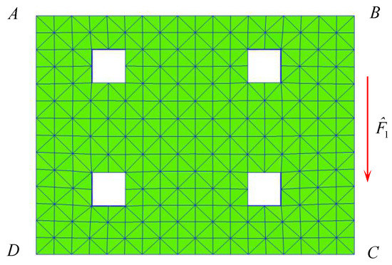
Figure 2.
A perforated rectangular plate loaded with downward load .
- (3)
- ARIMA prediction.
ADF stationarity test the original data , the purpose is to test the stability of the current sequence. If , then the original sequence is nonstationary and needs differential processing. This method of forecasting is different from other methods. In the same way, a stationary sequence can be considered when . this practical example test the statistic stat = −2.4537, p Value = 0.01449, . So the sequence is an nonstationary sequences, It needs to process the original sequence by differential. Through multiple debugging and validation, the best parameter determined in this paper is ARIMA(2, 1, 2).
When the sequence changes from non-stationary to a stationary sequence through difference, the model is converted to an ARMA model, and then the model needs to be determined ordered. It can be judged by the AIC function. When value is the smallest, then this model parameters have obtained better parameters, and the AIC function is defined as follows:
Of course, autocorrelation function values can also be calculated according to the sequence quantification Formula (46), its range is .
The definition of partial autocorrelation coefficient is: for a stationary AR (P) sequence, the lagged k-order partial autocorrelation coefficient refers to the correlation of influence on under the condition of given intermediate k-1 random variables , that is, after taking out the interference of intermediate k-1 random variables. Let . And then, the calculation formula of partial autocorrelation coefficient is as as follows:
In Example 1, the corresponding stress, strain and displacement cloud map are calculated under and predictive force . Variable force is predicted by the ARIMA algorithm, and the predicted results are shown in Figure 3a is the result of the variable force prediction by the algorithm. The blue line represents the historical data, the red line represents the data predicted by ARIMA and the black line is the confidence interval of the predicted value. The second Figure 3b uses Ljung-box Q statistics to carry out white noise test, which mainly detects whether the measured random data are a white noise sequence. Stat is the Ljung-box Q statistic test statistic, C value means the threshold of the test. MATLAB software was used to calculate the Ljung-box Q test statistic Stat = 7.329, p Value = 0.0157, h = 1; all the results still show that the residual sequence is white noise sequence, and its characteristics are consistent with that of white noise. The model can be used for prediction. If the discrete points of the standard normal quantile are distributed on the red line, it indicates that this group of test data is effective and meets the basic solving requirements of the ARIMA algorithm. Figure 3c,d are autocorrelation graphs and partial autocorrelation graphs. Both of them are trailing, which shows that this example model is selected correctly.
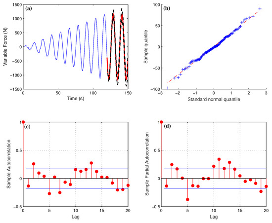
Figure 3.
(a) Prediction results of the ARIMA algorithm for variable forces . (b) Quantile Quantile (QQ) plot for normality test. (c) Time series auto-correlation function (ACF) plot of variable load. (d) Time series partial auto-correlation function (PACF) plot of variable load.
The optimal parameter selection for this example is ARIMA(2, 1, 2), the corresponding prediction model formula is:
It can also be written as follows:
Among them, the sequence value is a white noise sequence.
ARIMA model is mainly aimed at the prediction of nonstationary sequences. The nonstationary sequences can be processed into stationary sequences according to the difference method. The order method of the model is consistent with the order method of the ARMA model. The positive and negative sign represent the direction of the force in Table 2. The k order difference formula can be derived from first order difference , . Then, the parameters of Equation (48) to be estimated, which can be obtained based on the least squares, the estimated result is . The corresponding p values of t statistics are all less than 0.05, so the parameter estimation is significant using 100 historical data points to predict 30 data points backwards. The predictive force from to , which are shown in Table 2. Force can be generated according to function, the of which is a random disturbance term and .
Table 2.
ARIMA model and BP prediction results of variable force .
Here, we compared the predicted results by BP neural network and ARIMA method [55,56]. Neural networks is a mathematical model established from the simulation of human brain nervous system in microstructure and function. It has the ability to simulate human brain thinking. Its characteristics are mainly nonlinear characteristics, learning ability and adaptability. It is an important method to simulate human intelligence. The prediction results of ARIMA method and BP neural network are shown in Table 2 below.
From the predicted numerical results of Table 2 we can shown that the ARIMA model has more advantages. This example can better examine the superiority of the algorithm. Other linear regressions, nonlinear regressions and sequential minimal optimization (SMO) for SVR are basically unpredictable, because of the error is too large. Numerical conclusion: The common feature of the two methods is that the error will gradually accumulate with the increase in prediction time. This is because the ARIMA model uses a period of historical data iteration every time to produce error accumulation, and the BP neural network has larger prediction error and poor stability. This algorithm also verifies the effectiveness of the ARIMA algorithm.
- (4)
- Visualizing numerical results.
The prediction result is obtained by ARIMA algorithm, and then according to the energy equation and variational principle, and the solving process follows above Section 2. The solution steps are divided into: Load prediction, grid division, single stiffness matrix calculation, total stiffness matrix synthesis, finally, cloud image output. In order to better understand the internal material struct properties, stress distribution, and predict the deformation position. This article predicts the situation where the load is when time is . We calculate the corresponding physical quantities of stress, strain and displacement under four grid scales, and output the cloud map to facilitate user comparison and research.
As shown in Figure 4, the Figure 4a is the displacement of the x direction of the thin plate, Figure 4b is the displacement of the y direction. It is easy to distinguish the color that the left-end boundary is fixed, a right-end boundary is subjected to downward force . Figure 4c,d, respectively, represent the strain corresponding to the x direction and the y direction. The strain is obvious near the fixation location closer, and the more color, the more depth. The last two pictures in Figure 4e,f are the Von Mises stress and stress . Through the comparison of the above numerical results, the relationship between the physical quantities can be clearly identified, including the position of stress maximum and displacement maximum. Figure 4g is the strain on the mesh scale 1. Figure 4h is the numerical convergence rate of CST element. Before calculation, we need to emphasize that there is no analytical solution for the porous elastic plate. The treatment method in this paper is to calculate the numerical solution on the finest mesh scale 4, and then the numerical solution is approximately regarded as an analytical solution. Compared with the numerical solution at other mesh scales, the corresponding error is calculated and the convergence rate is finally obtained. From the numerical results, the following conclusions can be obtained: the convergence rate of displacement is order 2 and the stress and strain basically meet the linear convergence. This conclusion is consistent with the theoretical convergence rate analysis, which verified the effectiveness of the numerical method ARIMA-FEM.

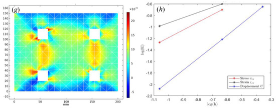
Figure 4.
(a) Displacement U on the scale mesh 1. (b) Displacement U on the scale mesh 2. (c) Displacement U on the scale mesh 3. (d) Displacement V on the scale mesh 2. (e) The numerical solution cloud map of Von Mises stress on the scale mesh 1. (f) The numerical solution stress of perforated rectangular plate on the scale mesh 1. Stress analysis of perforated rectangular plate under predictive force . (g). The strain tensor on the scale mesh 1. (h). The convergence rate of CST element.
4.2. Example 2
- (1)
- Basic parameters of the material.
This example is mainly to demonstrate an analysis on a square thin plate with an oval hole under the predicted variable force . The difference between Example 2 and Example 1 are the plate shape. The material parameters of square plate are as follows: length , width and thickness of steel plate. The distance of elliptical long axis a is , short axis b is 5 mm. Elastic modulus and Poisson’s ratio boundary conditions: the upper boundary AB and the lower boundary CD are free edges, and the left boundary AC is fixed.
The right boundary is subjected to the horizontal rightward force , the boundary condition of the external force on the edge can also be expressed as:
The LST element is used to discretize the square metal plate with elliptical holes. Each triangular element has six nodes, and the nodes on the midpoint of the edge are not displayed. The mesh generation and boundary application are shown in Figure 5:
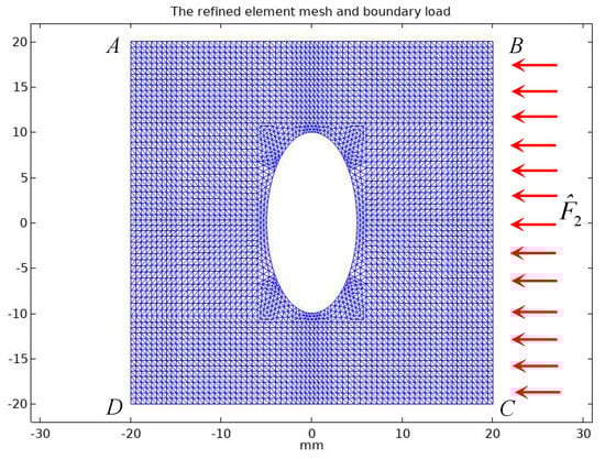
Figure 5.
Predictive force loaded on the square plates with elliptical hole.
The ARIMA algorithm prediction the force, the direction of the force does not change. The force can generate historical test data according to the , where the is a random term and . 50 variable force data generated by when the . Our purpose is to predict five data points backwards by ARIMA prediction algorithm.
- (2)
- Mesh subdivision.
Using the six-node LST element to discrete the square thin plate with oval hole, and the number of elements is , and the nodes , per element . The total number of degrees of freedom is 17,244. The above data information is conducive to the solution of finite element elastic equations, which can transform differential equations into algebraic, as seen in Equation (53). ARIMA model can be used to predict the variable force . The time series of this example need to be transformed an stationary series, k order difference formula is:
Then, according to the reference , the significant level, variance and standard deviation are small, and the calculated results can be within the accepted range. ARIMA(2, 2, 3) is the best parameter for this prediction. We predicted 30 data points, and selected six representative prediction points show in Table 3.
Table 3.
Prediction results and relative error of variable force .
When the sequence changes from non-stationary to stationary sequence through difference, the model is converted to the ARIMA(p, q) model, and then the model needs to be ordered. In addition to the ordering method, it can also be judged by the function.
When p = 2, q = 2, the 545.31 is small relative to other parameters, which indicates the best value at this time. The formula for model ARIMA(2, 2, 2) can be abbreviated as:
Meanwhile, we can easily obtain the equivalent form:
Finally, the parameter value can be obtained by least squares estimation. After t-statistic test, the parameter estimation is significantly effective, the estimated result is:
This example is compared with the other three methods, namely BP prediction, linear regression and nonlinear regression (polynomial regression). Here, we give a short brief introduction to BP algorithm. Network initialization, according to the input and the expected output , the number of neurons ( nodes ) in the input layer, hidden layer and output layer of the network is determined. The connection weights , between neurons in each layer are initialized, the hidden layer threshold a and the output layer threshold b are initialized and the learning rate and the neuron transfer function are given.
In Equation (59), m is the mumber of hidden layer nodes, function is a implicit layer transfer. According to the hidden layer output , connecting weights and thresholds b, the actual output prediction value of BP neural network is calculated.
Then, the total error of computing network is as follows:
During each iteration, is the reference value, is the current network prediction value. the BP method need to update the network connection weight to determine whether the iteration ends. Similarly, the expression of linear regression model is used to predict some load, the goodness of fit , root mean square error RMSE = 141.4, the linear regression expression is as follows:
Nonlinear regression model is mainly quadratic polynomial fitting historical load data, through the least squares equation to estimate the parameters. The goodness of fit , root mean square error RMSE = 141.2, the expression of quadratic polynomial is Formula (62):
Now, the ARIMA forecasting model has been established, the prediction results and errors are shown in Table 3. By comparison, it is easy to find that ARIMA is the best of the four prediction methods. From Table 3, we can draw a conclusion: both ARIMA and BP predictions decrease slightly as the prediction interval becomes longer. Although the error range of linear and nonlinear predictions is relatively stable, the approximation accuracy is relatively low. Therefore, The numerical comparison results show that ARIMA predicts the variable force relatively well.
- (4)
- Test of ARIMA prediction results.
The prediction result was by the ARIMA algorithm, and then according to the energy equation and variational principle, it is easy to obtain the equilibrium equation [48,49,50]. In Example 2, the corresponding stress, strain and displacement cloud are calculated under s and predictive force N. The solution process is the same as Section 2. The solution process is divided into the following steps: load prediction, solving domain meshing, discretization of linear elastic equations, solution of algebraic equations and output of cloud map results. The advantage of the numerical solution is that it can save a lot of experiments and provide a reference for decision making. The cloud map can also intuitively distinguish the position and size of mechanical changes.
From the prediction results in Table 3, we can see that the relative error of this ARIMA algorithm is small, and the approximation effect is very good. The analysis of stress, strain and displacement is meaningful, and the change of predicted mechanical behavior is more valuable. When t = 10.82, Example 2 selects the prediction load in order to calculate the stress, strain and displacement change of the thin plate under the side load with . The visualization of the prediction results is shown in Figure 6a, where the blue line is the original data and red points are the prediction data. Figure 6b is the standard normal test of the data. If the blue sample data points are concentrated near the red line, this shows that the sequence is normally distributed. Figure 6c is the autocorrelation coefficient map, and Figure 6d is the partial correlation coefficient map. Both autocorrelation data and partial autocorrelation data fall within the range of two standard deviations, and both graphs are truncated, indicating that the ARIMA model is correct.
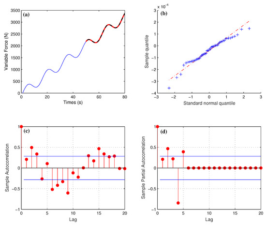
Figure 6.
(a) Prediction results of the ARIMA algorithm for variable forces . (b) Quantile Quantile (QQ) plot for normality test. (c) Time series auto-correlation function (ACF) plot of variable load. (d) Time series partial auto-correlation function (PACF) plot of variable load.
- (5)
- Visualization of numerical results.
Von Mises is a yield criterion whose value is usually called equivalent stress. It uses stress contour to represent the stress distribution inside the model so that analysts can quickly determine the most dangerous area in the model. Under certain conditions, when the second invariant of the stress deviatoric tension of a point in the stressed object reaches a certain value, the point begins to enter the plastic state, namely
The expression of principal stress is:
where is the yield point of material, K is a shear yield strength of material, and the 3D equivalent stress can be obtained by combining Equations (63) and (64):
Similarly, the Von Mises stress expression of two-dimensional elastic plate is:
Therefore, the physical meaning of Von Mises stress criterion is that under certain deformation conditions, when the equivalent stress of a point in the stressed object reaches a certain value, the point enters the plastic state. Numerical results for eight subgraphs of Figure 6a are predicted at t = 10.82 s. According to the prediction error results of various models, the shorter the prediction time is, the higher the accuracy is, and the longer the prediction time is, the lower the accuracy is, which is related to the error accumulation. This example solves a stress, strain and displacement of a square plate with an oval hole, where the left side is fixed and the right boundary is subjected to a horizontal rightward force . The variable force can be predicted by the ARIMA algorithm, and the thin plate area is discretized using six-node LST elements. Figure 7a is a cloud map of the component u displaced along the x direction, and Figure 7b shift along the component v in the y direction. Figure 7c is the cloud map of strain , Figure 7d is strain and the changes are more obvious at both ends of the ellipse.
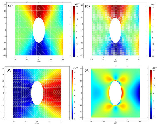
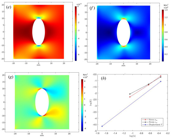
Figure 7.
(a) Displacement U on the scale mesh 1. (b) Displacement U on the scale mesh 3. (c) Displacement V on the scale mesh 2. (d) The strain tensor on the scale mesh 3. (e) The strain tensor on the scale mesh 3. (f) Von Mises stress on the scale mesh 3. (g) The stress tensor on the scale mesh 3. (h) The numerical convergence rate of LST element.
Figure 7e is the cloud map of stress of the square plate. Figure 7f is the Von Mises stress of the square plate—it is a yield criterion whose value is commonly referred to as an equivalent stress. The benefit of the visualization of numerical solutions lies in the convenience of comparison and is easier to find dramatically changing locations. Figure 7g is the cloud map of strain on the mesh scale 3, this graph is different from the strain in x direction and y direction, it does not have symmetry. Figure 7h is the numerical convergence rate of square plate with elliptical holes. The conclusion obtained by numerical calculation is that the LST element is used for regional discretization and solution of the linear elastic thin plate, and the numerical convergence order of displacement is close to 3. Stress and strain have the characteristics of second-order convergence, which is obviously faster than that of the CST element.
4.3. Example 3
- (1)
- Boundary conditions and material parameters.
Firstly, this example need to predict the force in a center hole disc, it is also a very common part in actual industrial processing. For example, in a variable acceleration bearing section, pressure vessel radial section, expansion bolt section and so on [57,58]. As for the symmetry of the circular plate, it is only necessary to analyze the 1/4 part. Here, in order to compare the force changes of the entire disc, we have solved the linear elastic equation for the entire disc [51]. The accurate stress analysis of the thin disc plate can improve the industrial design technology, optimize the geometric structure of the material and improve the quality of the product. Geometric parameters: The radius of the disc and the radius of the inner circular hole . The thin plate thickness is , Elastic Young’s modulus , Poisson ratio .
- (2)
- Boundary conditions.
For the center hole disc, this calculation example has two boundaries [59], the inner boundary is the edge of the inner circular hole and the outer boundary is the edge . The outer boundary is fixed and its displacement boundary condition is denoted as:
The inner boundary is subjected to a varying load , the value of can be predicted by the ARIMA algorithm. When the , the inner boundary is subjected to a uniform outward force , the prediction force is . The schematic diagram of adding load on the inner boundary is shown in Figure 8a, the boundary equation from Equations (68) to (70).
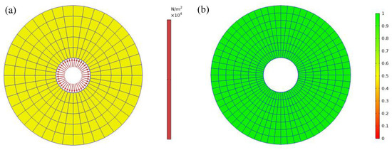
Figure 8.
Added boundary load and mesh quality assessment: (a) Boundary load of a disc with center circle hole. (b) Mesh quality of a disc with center circle hole.
- (3)
- Mesh subdivision.
The element division of the fan plate is different from Example 1 and Example 2. Due to Example 1 and Example 2 mainly adopting the triangular element, the shape of the Q4 element includes: square, rectangular and isoscelisted trapezoids. For geometric models of the thin disk shape, this paper employs quadrangle Q4 elements for discrete, and the mesh needs two steps to implement.
First of all, we need to divide the central angle , , which indicates that the circumference have been divided into n equal parts, and then, choose arbitrary radius and divide it into m equal parts and form m concentric circles. Then, the quadrangle mesh is generated. The total number of mesh nodes is , the total number of element is and of freedom per element. So, the total number of degrees of freedom is , the maximum of the element side length such that , . Figure 8a adds a uniform load to the center hole and Figure 8b is a mesh quality evaluation diagram.
- (4)
- Force prediction.
The forces can generate historical test data based on . Among them, , and random term is . Then, the ADF test is also required, with reference to determine the significance level [60,61,62]. Small variance and standard deviation and the calculated result values can be within the accepted range. The optimal parameters of this example are set as ARIMA(2, 3, 2), the non-stationary time series is converted to stationary time series after d = 3 which represents three order difference operations. The order determination method of the model is consistent with that of the ARIMA model. The three-order backward difference formula is:
When p = 2, d = 3, q = 2, the = 465.13 is small relative to other parameters, which indicates the best value at this time. The formula for model ARIMA(2, 3, 2) can be abbreviated as:
Meanwhile, we can easily obtain the specific Equation (73) forms of :
Finally, The parameter value can be obtained by least squares estimation. After t-statistic test, the parameter estimation is significantly effective, the estimated result is:
Similarly, the expression of linear regression model is used to predict some load, the goodness of fit , root mean square error RMSE = 52.75, the linear regression expression is as follows:
Nonlinear regression model is mainly quadratic polynomial fitting historical load data, through the least squares equation to estimate the parameters. The goodness of fit , root mean square error RMSE = 53.31, the expression of quadratic polynomial is Formula (76):
Then the ARIMA forecasting model has been established, the variable force data can be predicted backwards 20 s by the ARIMA algorithm, we have selected five representative forecast datasets to display and include errors are shown in Table 4:
Table 4.
Prediction results and relative error of variable force .
As predicted results in Table 4, the ARIMA relative error of prediction data remains at ∼, among the four prediction methods, ARIMA still has the best prediction effect. We estimate the variable force load data with trend and large fluctuation; the prediction variable force at s; the corresponding variable force load output by ; output the stress, strain, displacement cloud map and the predicted mechanical behavior to have a more meaningful reference. The ARIMA prediction results and parameter test diagram are as follows:
The prediction result of the ARIMA algorithm for the variable force in Figure 9a, blue curve represents the historical load data information, and the red curve is the predicted load value. The original numerical sequence has a decreasing trend with small waves, so it is necessary to make it become a differential stationary sequence.
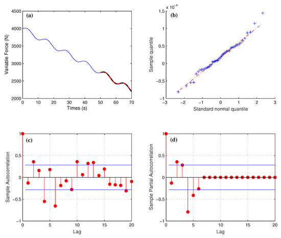
Figure 9.
(a) Prediction results of the ARIMA algorithm for variable forces . (b) Quantile Quantile (QQ) plot for normality test. (c) Time series auto-correlation function (ACF) plot of variable load . (d) Time series partial auto-correlation function (PACF) plot of variable load .
Figure 9b: We can see that the blue points are concentrated around the red line, the QQ chart can show that the selected set of data obeys a normal distribution, and these points in the chart are indeed on the diagonal line, indicating that the analysis model is reasonable and the observed value of p value should be consistent with the expected value. When the points on the QQ diagram are approximately near a straight line, it can be considered that the model residual is in line with the normal distribution. Moreover, the QQ diagram can also obtain the rough information of the skewness and kurtosis of the sample data. If the randomness and independence of the observed values in a certain period of time are observed, it can be combined with the Ljung-Box test. Figure 9c is the autocorrelation function and Figure 9d is the partial correlation function. They can be used to judge whether the data are truncated or trailed, and the data in the two graphs are basically within two times the standard deviation range, so they are all truncated. It is correct to choose the ARIMA model using AIC or BIC to determine the model parameters p, q. The conclusion obtained by numerical calculation is that the Q4 element is used for regional discretization and solution of the linear elastic thin plate, and the obtained displacement numerical convergence order is close to 2. The stress and strain have the characteristics of linear convergence, and the convergence rate is close to that of the CST element.
Variable force is the prediction by the ARIMA algorithm. Then the mechanical equations of the disc are solved by the FEM theory of Q4 element. Finally, a large sparse linear equation is solved, and the corresponding physical quantities such as displacement, stress and strain are obtained. In addition to the stress , the stressed objects also have the horizontal shear stress and the oblique surface shear stress , we can establish a balance equation, which can be obtained:
Equation (77) is a stress circle with the center and the radius . When , we can obtain the first and second principal stress values .
- (5)
- Visualization of numerical results.
Part of the numerical results for Example 3 are shown in Figure 10, which is generated under the predicted load . Example 3 mainly calculates the stress, strain and displacement of the disc by ARIMA-FEM algorithm at t = 54 s. Figure 10a,b correspond to the displacement in the x direction and y direction; the numerical variation of the void edge is obvious from the graph. Figure 10c,d are the strain in the and , respectively. Figure 10e is the stress of the circle plate on the scale mesh 1; Figure 10f is the first principal invariant of stress on the scale mesh 3. By comparing the above results, the relationship between the various physical quantities and the position of the maximum stress and displacement can be clearly distinguished. Regardless of stress or strain, the numerical change is relatively large close to the center circular hole. In addition, the circular plate visualization has good symmetry. Figure 10g is the stress on the scale mesh 3, the stress nephogram has obvious symmetry, which is greatly related to the uniform boundary load. Figure 10h is the convergence rate of bilinear element Q4. The conclusion obtained by numerical calculation is that the Q4 element is used for regional discretization and solution of the linear elastic thin plate, and the obtained displacement numerical convergence order is close to two. The stress and strain have the characteristics of linear convergence and the convergence rate is close to that of CST element.
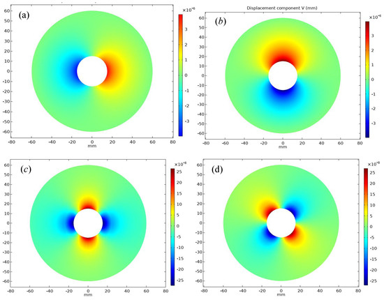

Figure 10.
(a) The displacement U on the scale mesh 3. (b) The displacement V on the scale mesh 3. (c) The strain tensor on the scale mesh 3. (d) The strain tensor on the scale mesh 3. Numerical results cloud map of circle thin plates: (e) The stress tensor on the scale mesh 1. (f) The first principal invariant of stress () on the scale mesh 3. (g) The stress tensor on the scale mesh 3. (h) The convergence rate of bilinear element Q4.
5. Discussion
5.1. The Extension of ARIMA-FEM Model
The application range of ARIMA-FEM model proposed in this paper is suitable for the load problem of thin plate with variable loading, which is also different from other mechanical models. For example, the contact problem analysis of rolling bearings, the contact problem of piezoelectric material probe, the fatigue life analysis of vehicle hub bearing, gear contact problem and rigid body collision need to be solved by a nonlinear transient dynamic model. Those models are more complex, the process of interaction needs to be considered, the fatigue damage dynamic analysis needs to be considered and the multi-scale analysis needs to be combined if deeper research is needed. Therefore, the method proposed in this paper is only helpful for the stress prediction analysis of elastic thin plates, and is also an analytical basis for the contact problem. In addition, the three-dimensional variable force prediction of the porous elastic plate can also be considered, especially the prediction of the variable force data in a small interval. Using the FEM model of the transient elastic plate, the change of the internal mechanics of the plate can be dynamically described.
5.2. Comparison of Advantages and Disadvantages of ARIMA-FEM Method
- (1)
- The advantages of ARIMA-FEM algorithms are as follows:
- (1.a)
- The traditional FEM stress analysis has hysteresis, which can only analyze the mechanical properties of the material at the current moment, and cannot predict the future mechanical properties. Our method can more accurately predict the future changes in material properties, and the application range of this method is wider.
- (1.b)
- The ARIMA-FEM method is compared with the pure machine learning method for stress analysis. The machine learning method needs more training data, select the appropriate network types (such as LightGBM, LSTM, Wavenet, etc. [63,64]), select the loss function and adjust the parameters. In short, the results cannot be quickly calculated. The LSTM model needs to be combined with a GPU to improve the training speed. The ARIMA-FEM has a simple operation and high calculation efficiency.
- (1.c)
- Traditional linear fitting, nonlinear fitting, grey prediction, BP neural network and other methods can all be used for predictions. When the data change trend is relatively large, the effect of nonlinear fitting and grey prediction is very poor, which can only simply predict the large trend and the local change trend cannot be accurately described.
- (2)
- The disadvantages of ARIMA-FEM algorithms are as follows:
ARIMA is suitable for data with time series and an unclear periodicity (seasonality). Strictly speaking, there is no universal numerical method, and any numerical method has certain scope of application and conditions. There are many types of data in engineering, most of which are continuous data and discontinuous data, especially for the detection and prediction of fault data and noise data. Due to the variety of abnormal situations, fast changes and great difficulty in prediction, this kind of situation is not suitable for the ARIMA method. The SARIM method can also be used for data with periodic changes. The treatment effect is better than ARIMA.
- (3)
- The relationship between ARIMA and other models.
The seasonal auto regressive integrated moving average model is the periodic autoregressive differential moving average.The SARIMA model is a very good model for predicting periodic time series. The difference between ARIMA and ARMA is whether the sequence is stationary or not. The ARMA model is called autoregressive moving average models—ARMA(), which is the combination of the AR(p) and MA(q) model. The theoretical significance of the AR and MA models is that the AR(p) model often observes momentum and mean reversion effect. The MA(q) model attempts to explain the shock effect observed under white noise—it can also be considered an accident that affects the observation process. The weakness of the ARMA model is that it ignores the wave aggregation effect in most time series. Then, the nested relationship between the ARIMA model and other four methods is shown in Figure 11 as follows:
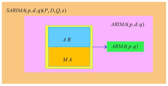
Figure 11.
The relationship diagram between ARIMA and other four models.
5.3. Superconvergence Analysis
In order to improve the convergence rate, we will discuss the related theory of p-type superconvergence method for solving linear elastic problems. Consider the 2D linear elasticity Equation (79).
Among them,
The stress tensor is defined as:
At the same time, the relationship between stress and displacement can also be expressed in the form of matrix tensor.
where and are Lamé parameters. The exact solution of displacement on discrete element is . The differential equation of Formula (79) can be simplified as:
Theoretically, the exact solution on the element can be obtained from this metamorphic problem, but the node displacement of the exact solution is unknown. When m > 1, in the process of mesh encryption, the node displacement of the element converges to the exact solution faster than the displacement of the inner point of the element [65,66]. Therefore, when the mesh is very dense, there is an approximate solution:
Such a boundary value problem in Formula (84) can be approximated to:
Then, the solution on the element can be approximated as by the solution of the boundary value problem. For the boundary value problem of Equation (86), the higher-order element is used to solve the finite element, so as to obtain the superconvergence solution on the element. The number of higher-order elements is denoted as , and the superconvergence solution on the element is denoted as:
The error between and is mainly caused by the disturbance of node displacement error at the end of the element, and the disturbance error is the same order as the node displacement error.
is the finite element solution of , the error is:
When m > 1, the convergence order of and is higher than that of , and it has superconvergence. Finally, the displacement is introduced into the original elastic Equation (79), and it can also be obtained:
6. Conclusions
This paper mainly studies the variable force prediction and simulation of two-dimen sional porous metal thin plates, which is also an application extension of 2D linear elastic problems. We combined the statistical prediction method and FEM method, it embodies the interdisciplinary application of multi disciplines. This method can obtain the mechanical property changes in advance, which is helpful for researchers to further evaluate and optimize materials. The conclusions of this paper are as follows:
- (1)
- We proposed an ARIMA-FEM algorithm, which combines the ARIMA algorithm with the FEM method. This method combines statistical prediction with the FEM to make the function more powerful.
- (2)
- In this paper, three numerical examples are given: the variable forces F1, F2 and F3 are predicted, respectively. Meanwhile, CST element, LST element and Q4 are successively used for discretization the thin porous metal plates.
- (3)
- Nonlinear bilateral filtering algorithm can preserve edge information and improve image quality. The cloud map of the stress, strain and displacement are output.
- (4)
- We give the error estimation and convergence analysis of the two-dimensional porous elastic plate. The numerical results show that the numerical convergence is basically consistent with the theoretical convergence, which verifies the effectiveness of the ARIMA-FEM method.
- (5)
- The application scope of ARIMA-FEM and the superconvergence analysis are discussed in depth. These works will be the objects to be studied in our future.
Porous metal plates have a variety of applications in life and industrial production, such as industrial parts, nanoscale filters, radiators, accelerated catalysis, mufflers and other materials. The method proposed in this paper can also promote the application of metal materials and the study of mechanical properties. Industrial processing of porous plates will be subject to different external forces in stamping. The method in this paper can predict deformation and stress. For metal filter net, it will also be affected by a different liquid impact; we can predict the load by recording historical data, combined with material corrosion and even predict the service life of the metal filter net. If the multi-physical field analysis is added, we can also study the thermal stress of porous metal plates during the heat dissipation and the change of heat flux during heat conduction. Multi-layer nano-metal thin plates combined with topological geometry can form a good muffler material. Finally, due to the good permeability of porous metal plates, the contact area of the catalyst can be increased and the reaction speed can be improved; therefore, a porous metal plate material is also a very interesting and useful research topic. Our research can also promote mechanical analysis and numerical simulation work in this field.
Author Contributions
Conceptualization, W.C., S.D. and B.Z.; methodology and experiments, W.C.; writing—original draft preparation, W.C.; writing—review and editing, W.C. and S.D.; visualization, W.C.; supervision, B.Z. and S.D.; funding acquisition, S.D. All authors have read and agreed to the published version of the manuscript.
Funding
This research was funded by the Science and Technology Major Project of Hubei Province under Grant 2021AAA010, and by the National Natural Science Foundation of China (Grant No. 12071363).
Institutional Review Board Statement
Not applicable.
Informed Consent Statement
Informed consent was obtained from all subjects involved in the study.
Data Availability Statement
Data for this article can be accessed publicly.
Acknowledgments
This research was funded by the Science and Technology Major Project of Hubei Province under Grant 2021AAA010, and by the National Natural Science Foundation of China (Grant No. 12071363). At last, we extend our thanks to the anonymous reviewers for their professional advice.
Conflicts of Interest
The authors declare that they have no known competing financial interest or personal relationship that could have appeared to influence the work reported in this paper.
References
- Sharma, P.; Dell, J.; Parish, G.; Keating, A. Engineering 1/f noise in porous silicon thin films for thermal sensing applications. Microporous Mesoporous Mater. 2021, 324, 111302. [Google Scholar] [CrossRef]
- Chaitanya, P.; Joseph, P.; Chong, T.P.; Priddin, M.; Ayton, L. On the noise reduction mechanisms of porous aerofoil leading edges. J. Sound Vib. 2020, 485, 115574. [Google Scholar] [CrossRef]
- Bhatti, M.M.; Arain, M.B.; Zeeshan, A.; Ellahi, R.; Doranehgard, M.H. Swimming of Gyrotactic Microorganism in MHD Williamson nanofluid flow between rotating circular plates embedded in porous medium: Application of thermal energy storage. J. Energy Storage 2021, 45, 103511. [Google Scholar] [CrossRef]
- Yun, J.; Shin, H.R.; Won, E.-S.; Kang, H.C.; Lee, J.-W. Confined Li metal storage in porous carbon frameworks promoted by strong Li–substrate interaction. Chem. Eng. J. 2022, 430, 132897. [Google Scholar] [CrossRef]
- Rodriguez-Contreras, A.; Punset, M.; Calero, J.A.; Gil, F.J.; Ruperez, E.; Manero, J.M. Powder metallurgy with space holder for porous titanium implants: A review. J. Mater. Sci. Technol. 2021, 76, 129–149. [Google Scholar] [CrossRef]
- Singh, H.; Saxena, P.; Puri, Y.M. The manufacturing and applications of the porous metal membranes: A critical review. CIRP J. Manuf. Sci. Technol. 2021, 33, 339–368. [Google Scholar] [CrossRef]
- Nickolay, A.L.; Eugene, A.S. Numerical modeling of heterogeneous combustion with phase transitions in porous metal-containing media. Int. J. Multiph. Flow 2021, 140, 103670. [Google Scholar]
- Chen, Z.; Zi, Z.; Zhou, T.; Wu, Y. Axial compression stability of thin double-steel-plate and concrete composite shear wall. Structures 2021, 34, 3866–3881. [Google Scholar] [CrossRef]
- Goodall, I.W.; Webster, G.A. Theoretical determination of reference stress for partially penetrating flaws in plates. Int. J. Press. Vessel. Pip. 2001, 78, 687–695. [Google Scholar] [CrossRef]
- Gong, J.; Xuan, L.; Ying, B.; Wang, H. Thermoelastic analysis of functionally graded porous materials with temperature-dependent properties by a staggered finite volume method. Compos. Struct. 2019, 224, 111071. [Google Scholar] [CrossRef]
- Ahmadi, F.; Ranji, A.R.; Nowruzi, H. Ultimate strength prediction of corroded plates with center-longitudinal crack using FEM and ANN. Ocean Eng. 2020, 206, 107281. [Google Scholar] [CrossRef]
- Ma, C.; Iijima, K.; Oka, M. Nonlinear waves in a floating thin elastic plate, predicted by a coupled SPH and FEM simulation and by an analytical solution. Ocean Eng. 2020, 204, 107243. [Google Scholar] [CrossRef]
- Zheng, F.; Han, X.; Hua, L.; Tan, R.; Zhang, W. A semi-analytical model for cutting force prediction in face-milling of spiral bevel gears. Mech. Mach. Theory 2021, 156, 104165. [Google Scholar] [CrossRef]
- Yan, S.; Kong, J.; Sun, Y. Continuum model based chatter stability prediction for highly flexible parts in turning process with accurate dynamic force modeling. J. Manuf. Process. 2021, 62, 221–233. [Google Scholar] [CrossRef]
- Zhou, T.; He, L.; Zou, Z.; Du, F.; Wu, J.; Tian, P. Three-dimensional turning force prediction based on hybrid finite element and predictive machining theory considering edge radius and nose radius. J. Manuf. Process. 2020, 58, 1304–1317. [Google Scholar] [CrossRef]
- Lian, P.; Liu, H.; Wang, X.; Guo, R. Soft sensor based on DBN-IPSO-SVR approach for rotor thermal deformation prediction of rotary air-preheater. Measurement 2020, 165, 108109. [Google Scholar] [CrossRef]
- Lecun, Y.; Bengio, Y. Hinton, Deep learning. Nature 2015, 521, 436–444. [Google Scholar] [CrossRef]
- Tao, L.; Guo, C.L. Network intrusion detection based on improved particle swarm optimization and support vector machine. Comput. Syst. Appl. 2016, 25, 269–273. [Google Scholar]
- Qiu, S.Y.; Yang, H.G. Assessment method of harmonic emission level based on the improved weighted support vector machine regression Trans. China Electrotech. Soc. 2016, 31, 85–90. [Google Scholar]
- Sadeghi, B. A BP-neural network predictor model for plastic injection molding process. J. Mater. Process. Technol. 2000, 103, 411–416. [Google Scholar] [CrossRef]
- Su, S.J.; Hu, Y.; Wang, C.F.; Liu, B. Hull Plate Bending Springback Prediction Based on Artificial Neural Network. Adv. Mater. Res. 2014, 988, 309–312. [Google Scholar] [CrossRef]
- Upendra, K.M.; Upadhyay, A. Buckling load prediction of laminated composite stiffened panels subjected to in-plane shear using artificial neural networks. Thin-Walled Struct. 2016, 102, 158–164. [Google Scholar]
- Ye, X.; Zhang, S.; Zhang, Z. A locking-free weak Galerkin finite element method for Reissner-Mindlin plate on polygonal meshes. Comput. Math. Appl. 2020, 80, 906–916. [Google Scholar] [CrossRef]
- Feng, F.; Han, W.; Huang, J. The virtual element method for an obstacle problem of a Kirchhoff-Love plate. Commun. Nonlinear Sci. Numer. Simul. 2021, 103, 106008. [Google Scholar] [CrossRef]
- Li, T.; Zhao, Y.; Xie, P.; Liu, B.; Qi, Y. Force prediction and influencing factors analysis of the coiled tubing blowout preventer in the shearing process. Eng. Fail. Anal. 2021, 121, 105073. [Google Scholar] [CrossRef]
- Serrano, B.; Infante, V.; Marado, B. Fatigue life time prediction of PoAF Epsilon TB-30 aircraft—Implementation of automatic crack growth based on 3D finite element method. Eng. Fail. Anal. 2013, 33, 17–28. [Google Scholar] [CrossRef]
- Sheil, B. Prediction of microtunnelling jacking forces using a probabilistic observational approach. Tunn. Undergr. Space Technol. 2021, 109, 103749. [Google Scholar] [CrossRef]
- Ala’raj, M.; Majdalawieh, M.; Nizamuddin, N. Modeling and forecasting of COVID-19 using a hybrid dynamic model based on SEIRD with ARIMA corrections. Infect. Dis. Model. 2021, 6, 98–111. [Google Scholar] [CrossRef] [PubMed]
- Pai, P.F.; Lin, C.S. A hybrid ARIMA and support vector machines model in stock price forecasting. Omega 2005, 33, 497–505. [Google Scholar] [CrossRef]
- Phan, T.; Hoai, N.X. Combining Statistical Machine Learning Models with ARIMA for Water Level Forecasting: The Case of the Red River. Adv. Water Resour. 2020, 142, 103656. [Google Scholar] [CrossRef]
- Salman, A.G.; Kanigoro, B. Visibility Forecasting Using Autoregressive Integrated Moving Average (ARIMA) Models. Procedia Comput. Sci. 2021, 179, 252–259. [Google Scholar] [CrossRef]
- Niu, M.; Sun, S.; Wu, J.; Zhang, Y. Short-Term Wind Speed Hybrid Forecasting Model Based on Bias Correcting Study and Its Application. Math. Probl. Eng. 2015, 2015, 351354. [Google Scholar] [CrossRef]
- Liu, M.-D.; Ding, L.; Bai, Y.-L. Application of hybrid model based on empirical mode decomposition, novel recurrent neural networks and the ARIMA to wind speed prediction. Energy Convers. Manag. 2021, 233, 113917. [Google Scholar] [CrossRef]
- Aasim; Singh, S.N.; Mohapatra, A. Repeated wavelet transform based ARIMA model for very short-term wind speed forecasting. Renew. Energy 2019, 136, 758–768. [Google Scholar] [CrossRef]
- Wang, Q.; Li, S.; Li, R.; Ma, M. Forecasting U.S. shale gas monthly production using a hybrid ARIMA and metabolic nonlinear grey model. Energy 2018, 160, 378–387. [Google Scholar] [CrossRef]
- Dasgupta, R.; Mandal, N.; Lee, C. Controls of subducting slab dip and age on the extensional versus compressional deformation in the overriding plate. Tectonophysics 2021, 801, 228716. [Google Scholar] [CrossRef]
- Yang, H.; Li, X.; Qiang, W.; Zhao, Y.; Zhang, W.; Tang, C. A network traffic forecasting method based on SA optimized ARIMA—BP neural network. Comput. Netw. 2021, 193, 108102. [Google Scholar] [CrossRef]
- Zhang, G.; Guo, T.F.; Elkhodary, K.I.; Tang, S.; Guo, X. Mixed Graph-FEM phase field modeling of fracture in plates and shells with nonlinearly elastic solids. Comput. Methods Appl. Mech. Eng. 2021, 2021, 114282. [Google Scholar] [CrossRef]
- Phan, N.D.; Reddy, J.N. Analysis of laminated composite plates using a higher order shear deformation theory with assumed strains. Lat. Am. J. Solids Struct. 2013, 10, 523–547. [Google Scholar]
- Cai, W.; Zhu, L.; Wang, F. Plastic deformation of ship plate subjected to repeated patch loads at different locations-Elastoplastic numerical analysis and design equation. Mar. Struct. 2020, 76, 102901. [Google Scholar] [CrossRef]
- Vinh, P.V. Modified single variable shear deformation plate theory for free vibration analysis of rectangular FGM plates. Structures 2020, 29, 1435–1444. [Google Scholar] [CrossRef]
- Tian, L.R.; Chen, F.L.; Zhu, L.; Yu, T.X. Large Deformation of Square Plates under Pulse Loading by Combined Saturation Analysis and Membrane Factor Methods. Int. J. Impact Eng. 2020, 140, 103546. [Google Scholar] [CrossRef]
- Amoushahi, H. Time depended deformation and buckling of viscoelastic thick plates by a fully discretized finite strip method using Third order shear deformation theory. Eur. J. Mech. A Solids 2018, 68, 38–52. [Google Scholar] [CrossRef]
- Khechai, A.; Tati, A.; Guerira, B.; Guettala, A.; Mohite, P.M. Strength degradation and stress analysis of composite plates with circular square and rectangular notches using digital image correlation. Compos. Struct. 2018, 185, 699–715. [Google Scholar] [CrossRef]
- Yao, Z. A new type of high-accuracy BEM and local stress analysis of real beam, plate and shell structures. Eng. Anal. Bound. Elem. 2016, 65, 1–17. [Google Scholar] [CrossRef]
- Marczak, J.; Michalak, B.; Wirowski, A. A multi-scale analysis of stress distribution in thin composite plates with dense system of ribs in two directions. Adv. Eng. Softw. 2021, 153, 102960. [Google Scholar] [CrossRef]
- Senthilkumar, D.; Arulmurugan, R. Gaussian bilateral filtered discrete Hartley feature transformation based infomax boosting for hyperspectral image classification. Int. J. Intell. Netw. 2021, 2, 195–203. [Google Scholar] [CrossRef]
- Li, X.; Zhou, F.; Tan, H.; Zhang, W.; Zhao, C. Multimodal medical image fusion based on joint bilateral filter and local gradient energy. Inf. Sci. 2021, 569, 302–325. [Google Scholar] [CrossRef]
- Xu, S. A posteriori error estimates for weak Galerkin methods for second order elliptic problems on polygonal meshes. Appl. Numer. Math. 2021, 161, 510–524. [Google Scholar] [CrossRef]
- Zhang, X.; Hu, Z.; Wang, M. An adaptive interpolation element free Galerkin method based on a posteriori error estimation of FEM for Poisson equation. Eng. Anal. Bound. Elem. 2021, 130, 186–195. [Google Scholar] [CrossRef]
- Guan, Z.; Wang, J.; Liu, Y.; Nie, Y. Unconditionally optimal convergence of a linearized Galerkin FEM for the nonlinear time-fractional mobile immobile transport equation. Appl. Numer. Math. 2022, 172, 133–156. [Google Scholar] [CrossRef]
- Wei, Y.; Lü, S.; Chen, H.; Zhao, Y.; Wang, F. Convergence analysis of the anisotropic FEM for 2D time fractional variable coefficient diffusion equations on graded meshes. Appl. Math. Lett. 2021, 111, 106604. [Google Scholar] [CrossRef]
- Saad-Eldeen, S.; Garbatov, Y.; Soares, C.G. Stress–strain analysis of dented rectangular plates subjected to uni-axial compressive loading. Eng. Struct. 2015, 99, 78–91. [Google Scholar] [CrossRef]
- Guenaneche, B.; Tounsi, A. Effect of shear deformation on interfacial stress analysis in plated beams under arbitrary loading. Int. J. Adhes. Adhes. 2014, 48, 1–13. [Google Scholar] [CrossRef]
- Bhuiyan, F.H.; Fertig, R.S. A PFA methodology to investigate UD composites in fatigue comprising a KTF-based model for matrix damage and stochastic fiber failure prediction. Compos. Struct. 2022, 279, 114724. [Google Scholar] [CrossRef]
- Wang, B.J.; Xie, S.Q.; Li, Q.; Ren, Z.S. Fatigue damage prediction of metro bogie frame based on measured loads. Int. J. Fatigue 2022, 154, 106532. [Google Scholar] [CrossRef]
- Cui, X.; Duan, S.Y.; Huo, S.H.; Liu, G.R. A high order cell-based smoothed finite element method using triangular and quadrilateral elements. Eng. Anal. Bound. Elem. 2021, 128, 133–148. [Google Scholar] [CrossRef]
- Kuznetsova, I.; Nedospasov, I.; Smirnov, A.; Qian, Z.-H.; Wang, B.; Dai, X.-I. Excitation and detection of evanescent acoustic waves in piezoelectric plates: Theoretical and 2D FEM modeling. Ultrasonics 2019, 99, 105961. [Google Scholar] [CrossRef]
- Webb, D.C.; Kormi, K.; Al-Hassani, S.T.S. Use of FEM in performance assessment of perforated plates subject to general loading conditions. Int. J. Press. Vessel. Pip. 1995, 64, 137–152. [Google Scholar] [CrossRef]
- Kim, H.-Y.; Ma, P.-Y.; Kim, B.-O.; Lee, S.-E.; Seo, Y.-U. Sound transmission loss of multi-layered elastic micro-perforated plates in an impedance tube. Appl. Acoust. 2020, 66, 107348. [Google Scholar] [CrossRef]
- Sheng, Z.Q.; Jirathearanat, S.; Altan, T. Adaptive FEM simulation for prediction of variable blank holder force in conical cup drawing. Int. J. Mach. Tools Manuf. 2004, 44, 487–494. [Google Scholar] [CrossRef]
- Pawlicki, J.; Głowacki, D.; Zwoliński, J.; Mościcki, A. Elastic limit load resource when reaming holes in turbine rotor discs. Eng. Fail. Anal. 2020, 13, 104555. [Google Scholar] [CrossRef]
- Hao, X.; Zhang, Z.; Xu, Q.; Huang, G.; Wang, K. Prediction of f-CaO content in cement clinker: A novel prediction method based on LightGBM and Bayesian optimization. Chemom. Intell. Lab. Syst. 2022, 220, 104461. [Google Scholar] [CrossRef]
- Cho, K.; Kim, Y. Improving streamflow prediction in the WRF-Hydro model with LSTM networks. J. Hydrol. 2022, 605, 127297. [Google Scholar] [CrossRef]
- Du, Y.; Wu, H.; Zhang, Z. Superconvergence analysis of linear FEM based on polynomial preserving recovery for Helmholtz equation with high wave number. J. Comput. Appl. Math. 2020, 372, 112731. [Google Scholar] [CrossRef]
- Wang, J. Superconvergence analysis of an energy stable scheme for nonlinear reaction-diffusion equation with BDF mixed FEM. Appl. Numer. Math. 2020, 153, 457–472. [Google Scholar] [CrossRef]
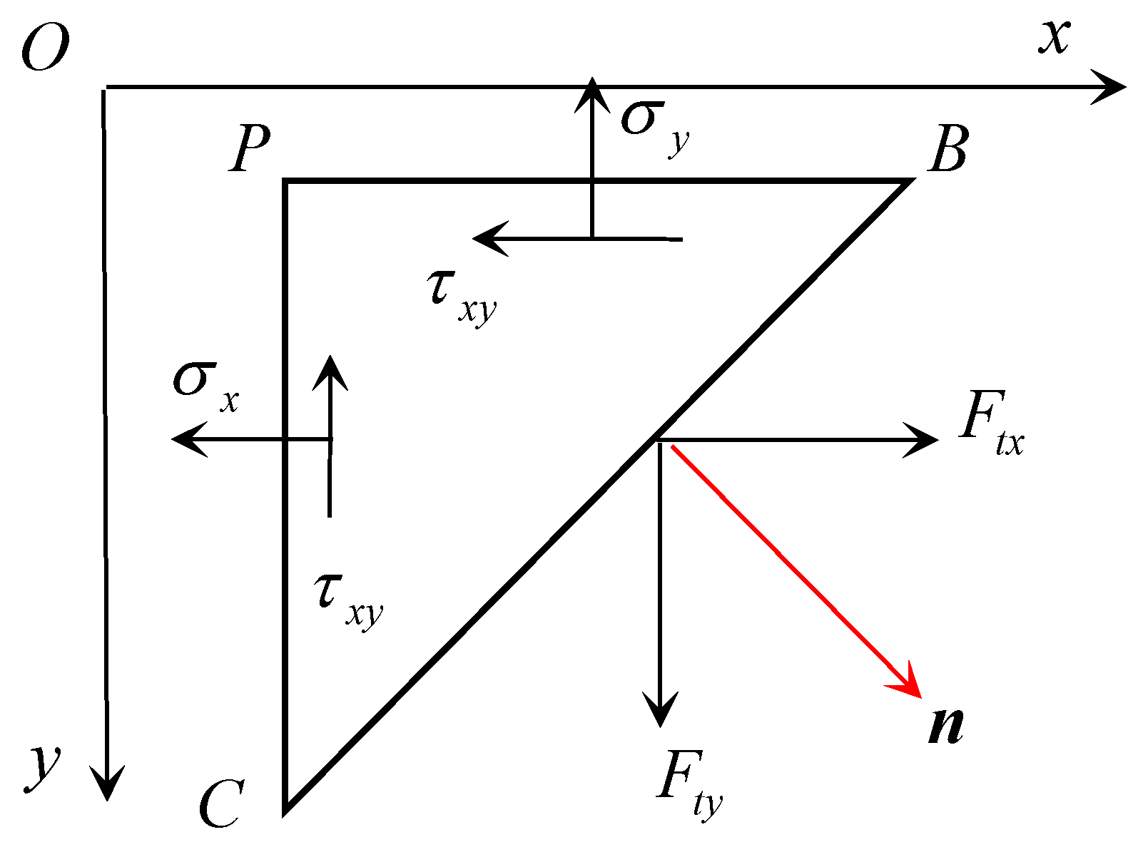
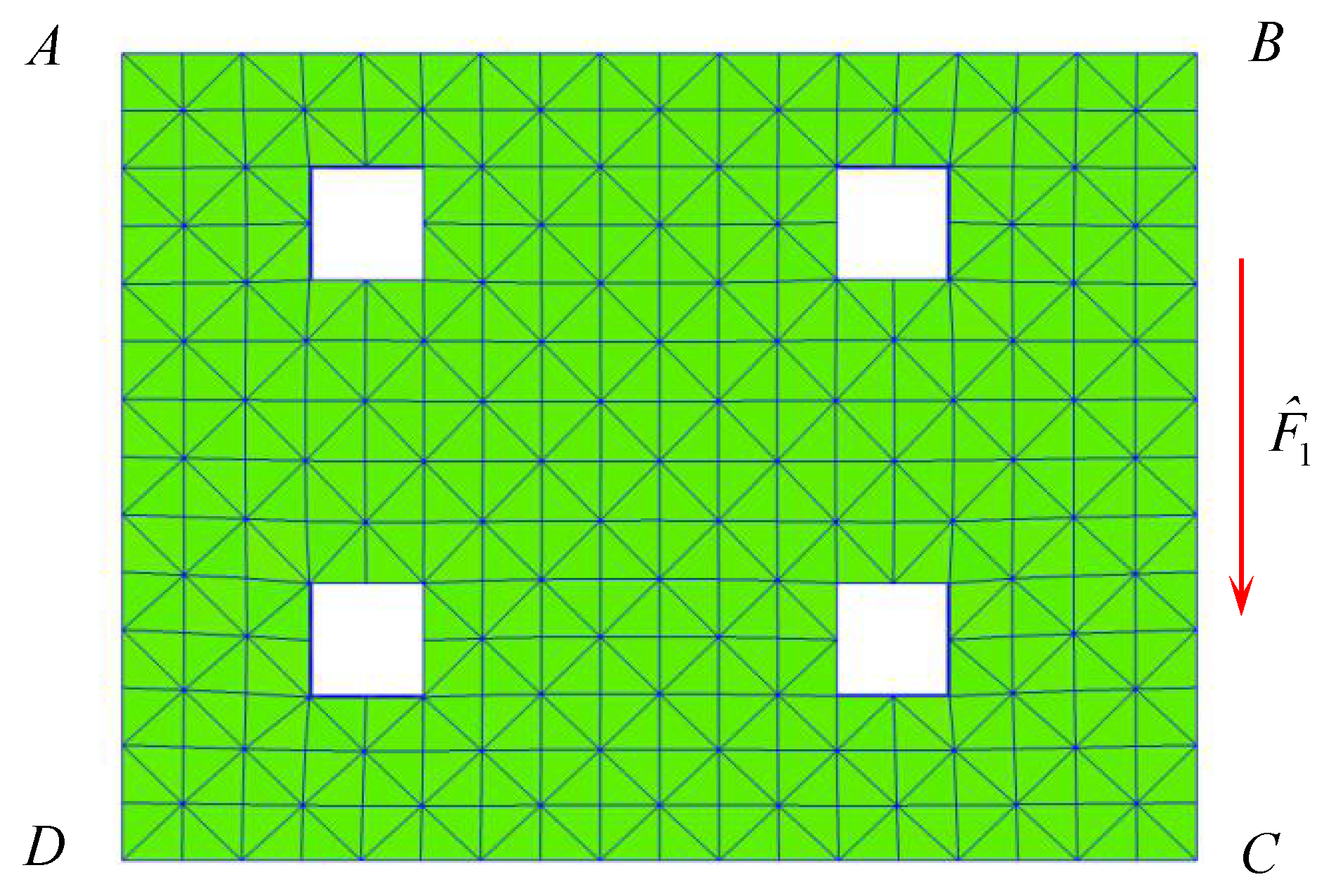
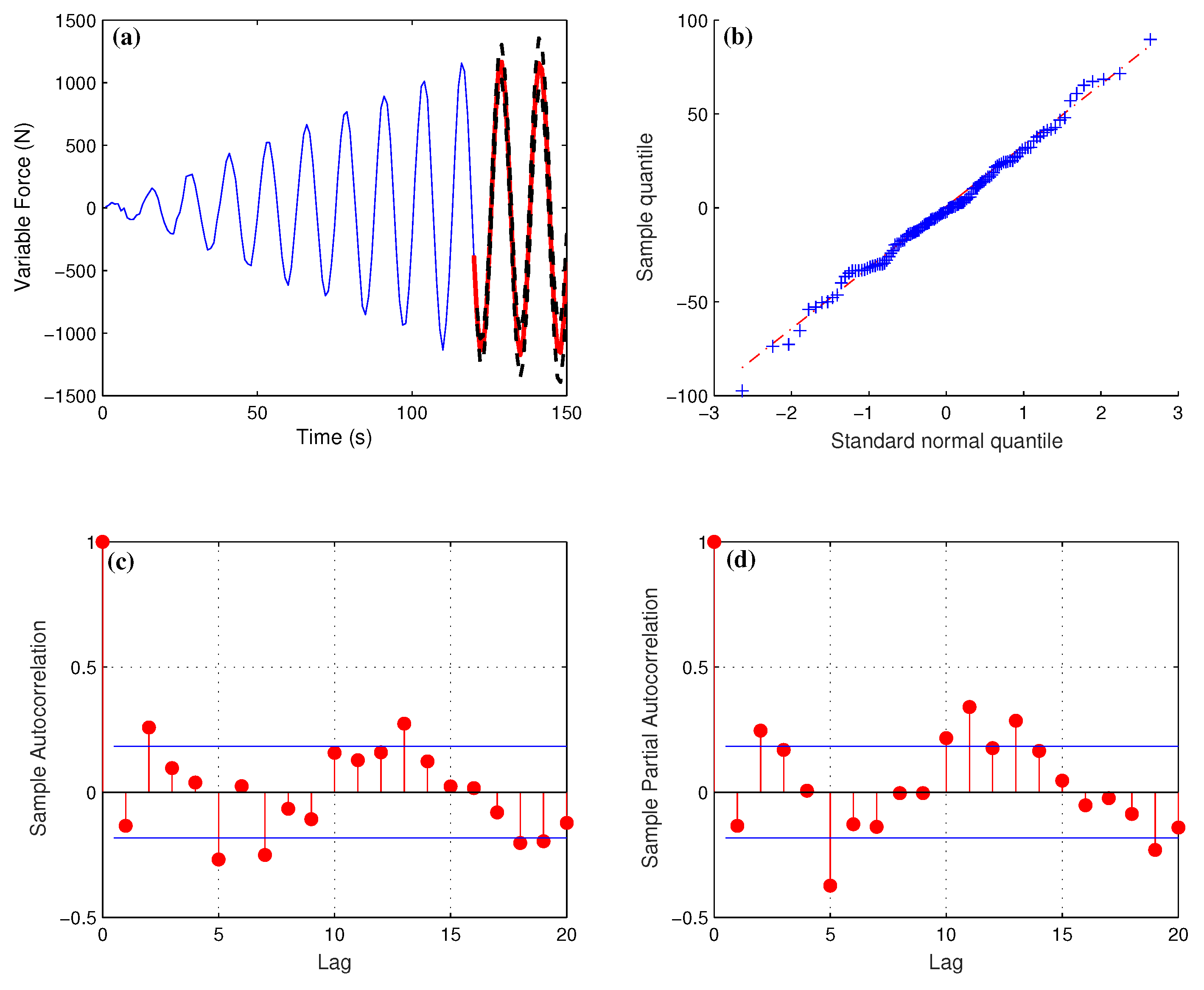
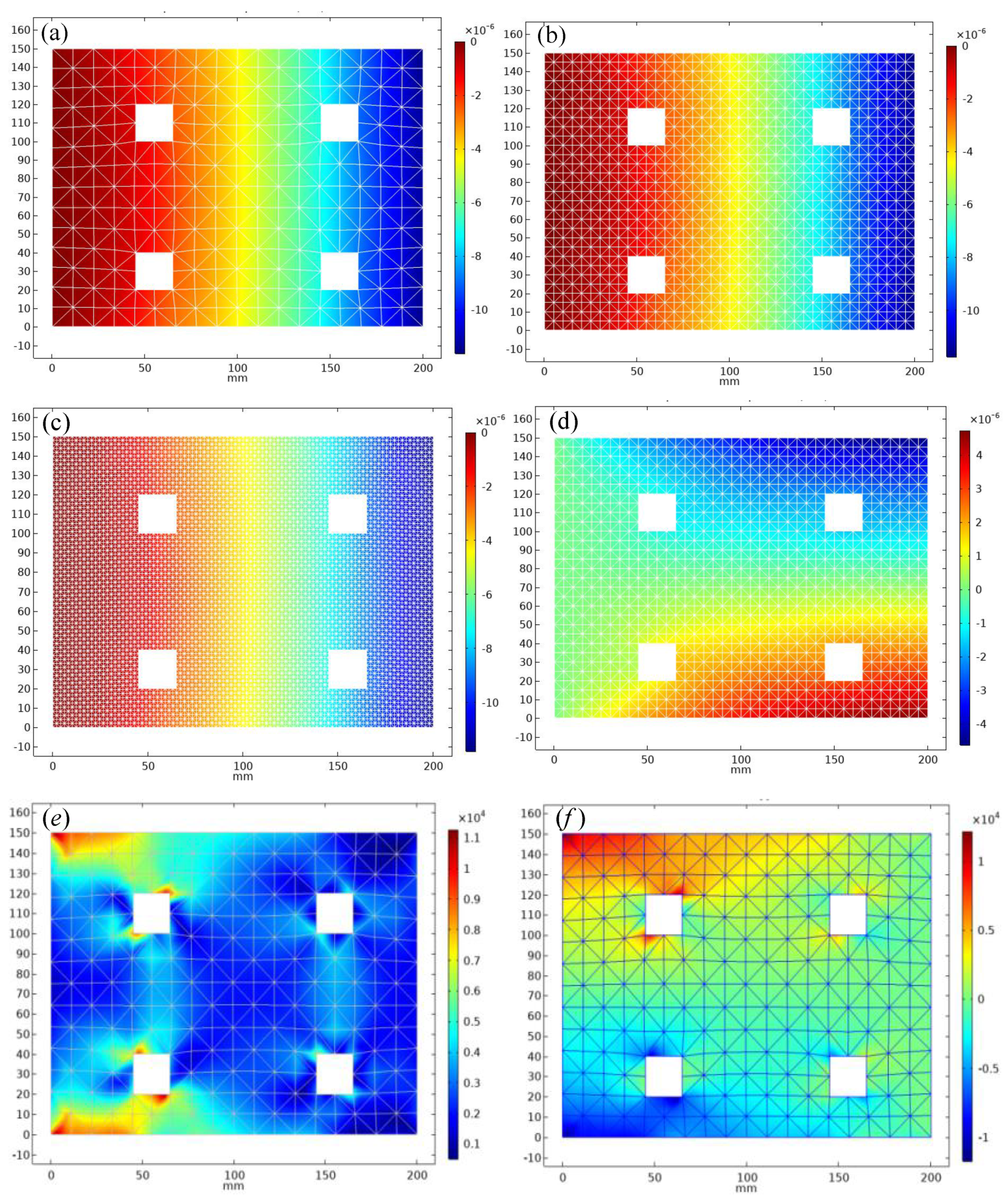

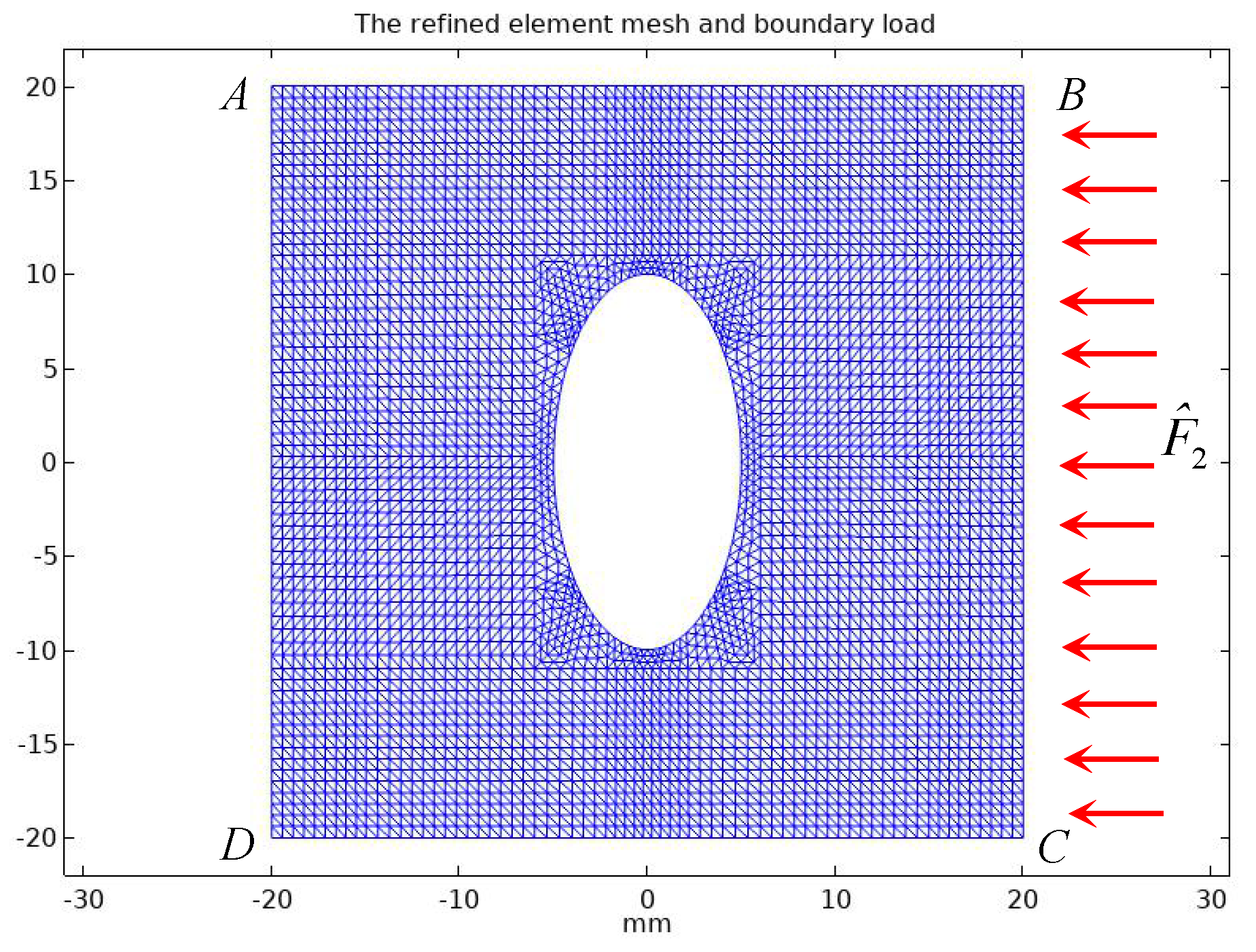
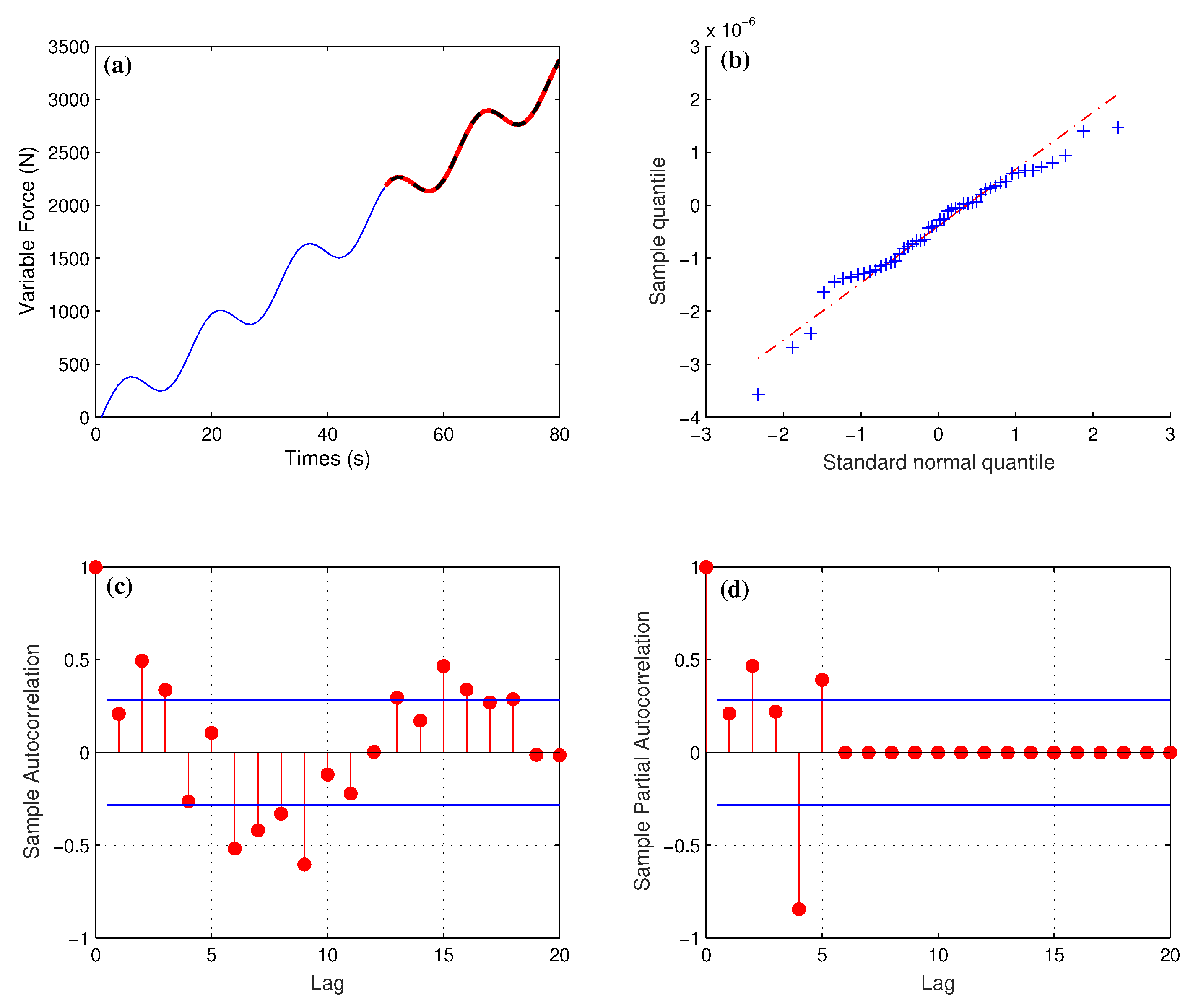


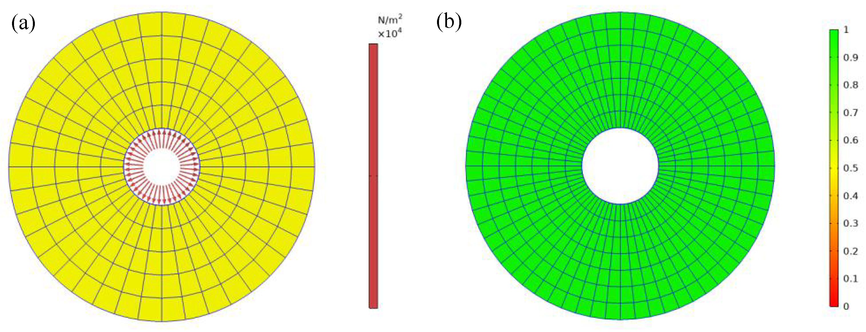
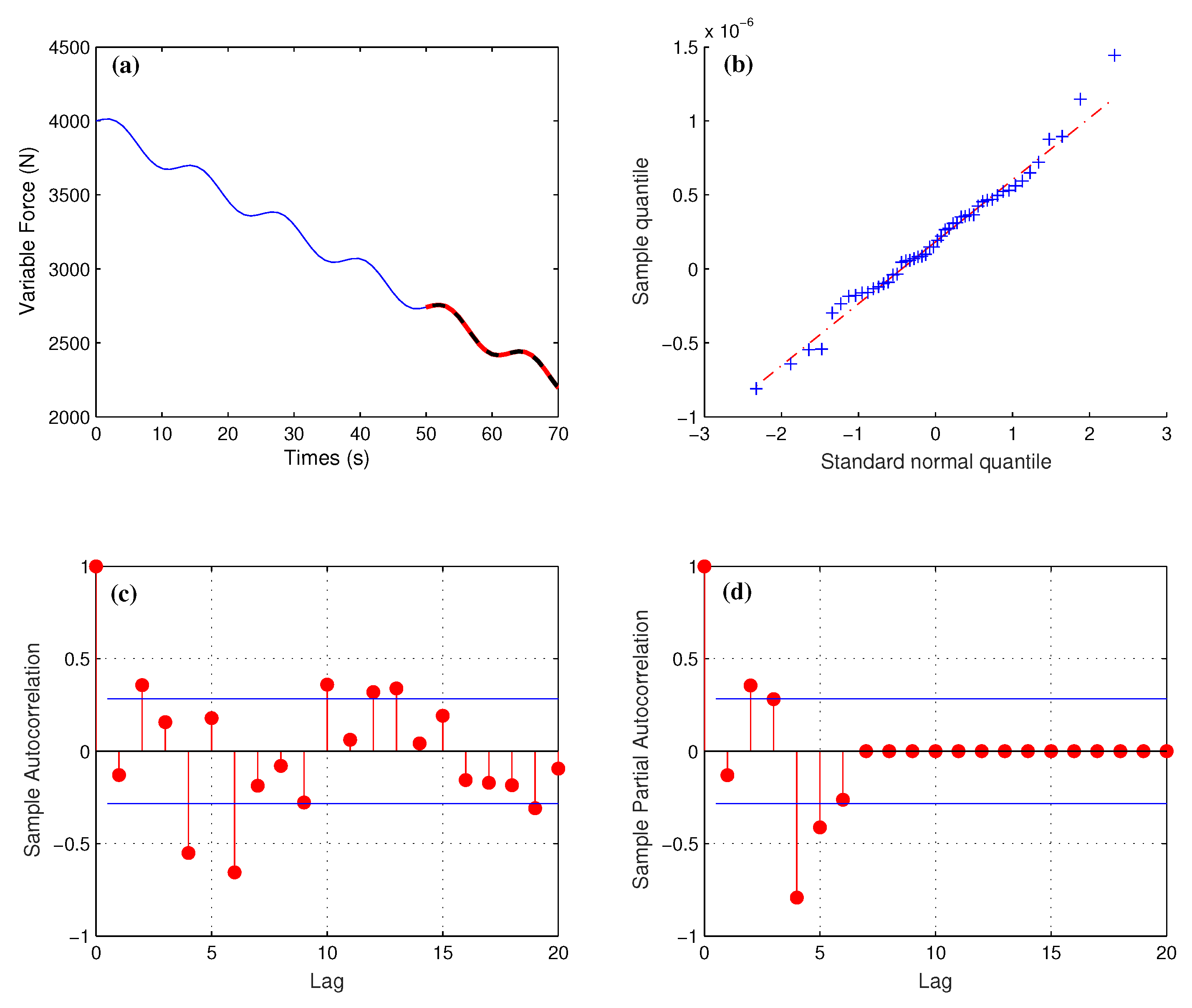
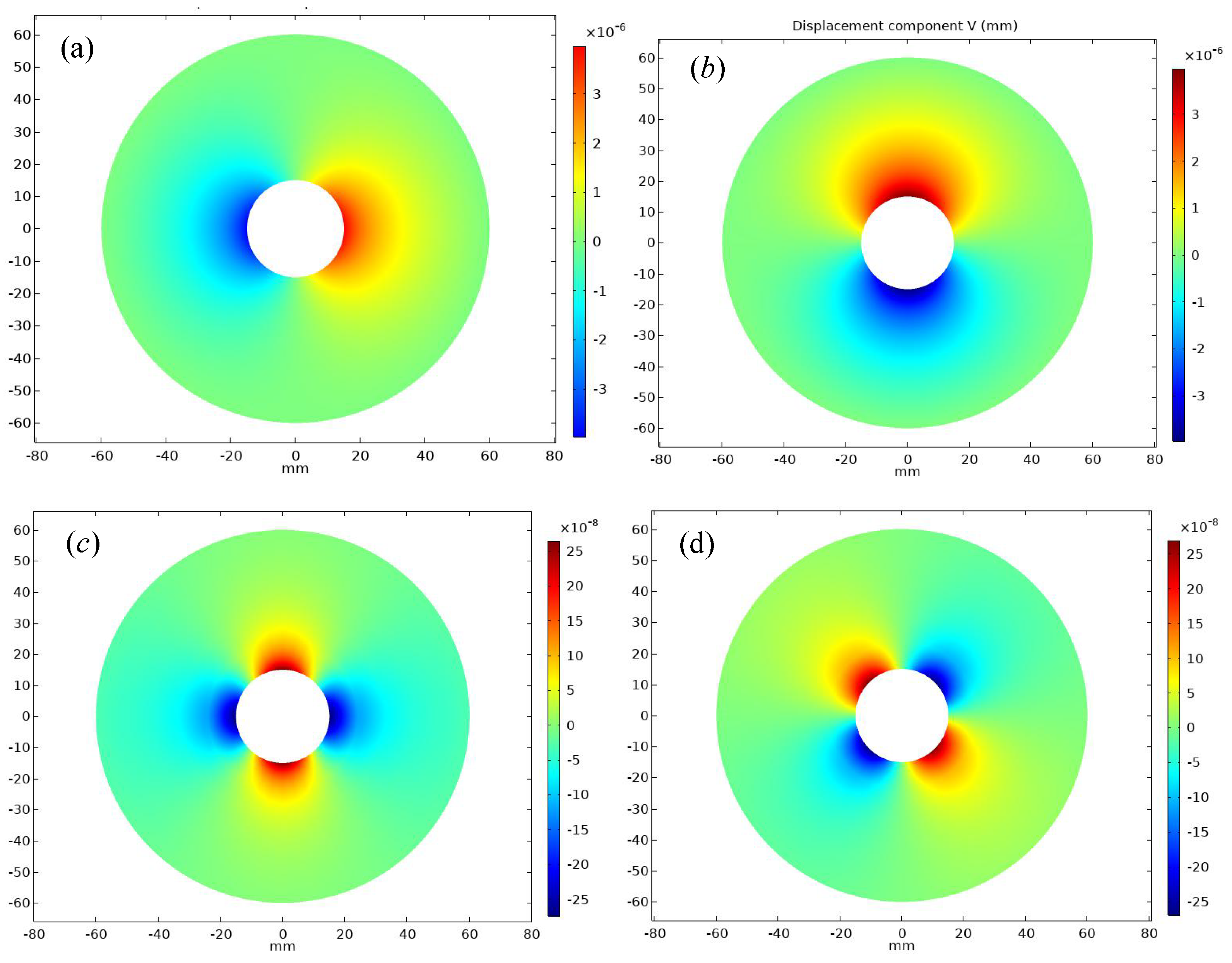
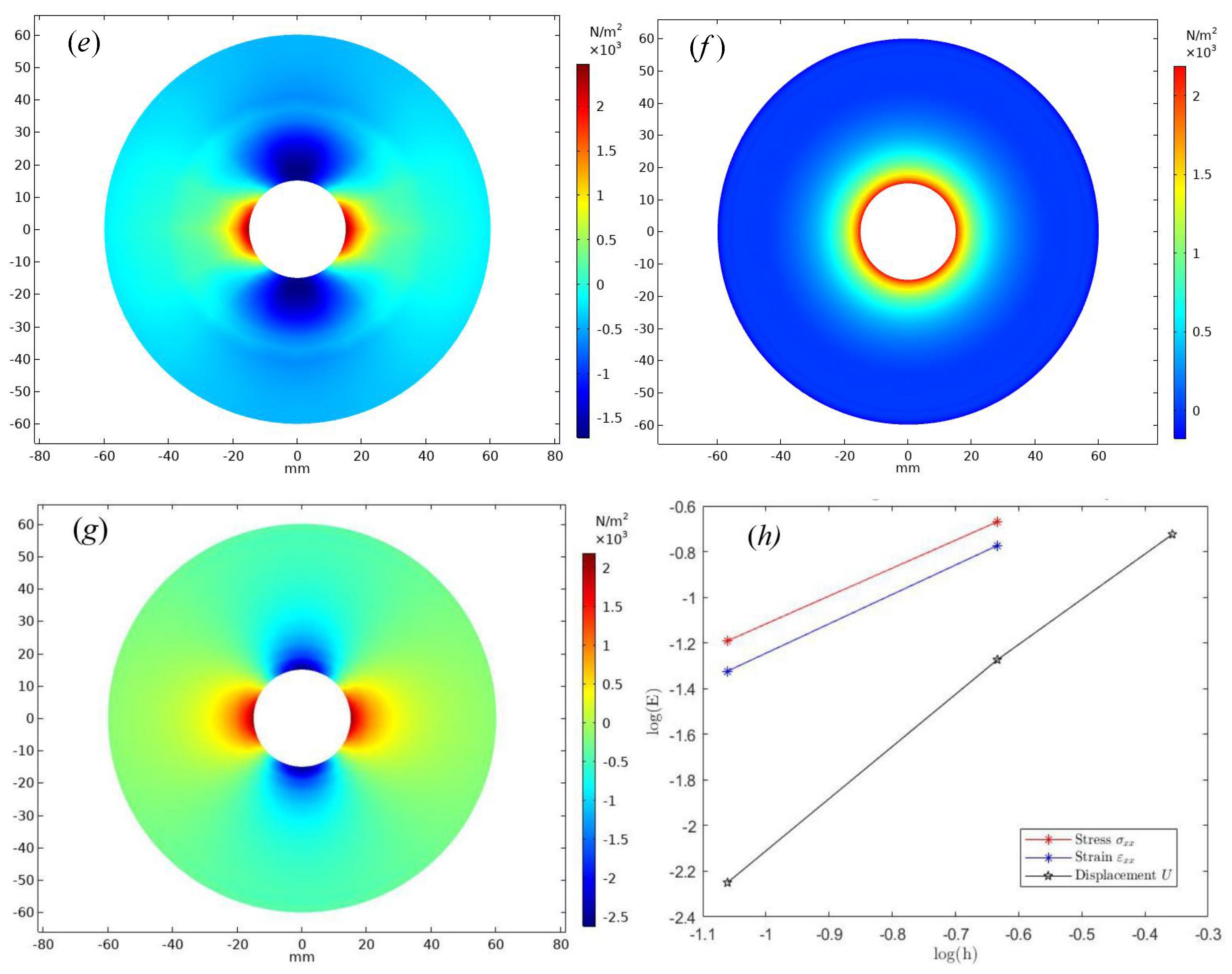

Publisher’s Note: MDPI stays neutral with regard to jurisdictional claims in published maps and institutional affiliations. |
© 2022 by the authors. Licensee MDPI, Basel, Switzerland. This article is an open access article distributed under the terms and conditions of the Creative Commons Attribution (CC BY) license (https://creativecommons.org/licenses/by/4.0/).