Article

Evaluation Method and Application of Cold Rolled Strip Flatness Quality Based on Multi-Objective Decision-Making

1
Hot Rolling Department of Qian’an Iron and Steel Corporation, Shougang Company Limited, Tangshan 064404, China
2
National Engineering Research Center of Flat Rolling Equipment, University of Science and Technology Beijing, Beijing 100083, China
*
Author to whom correspondence should be addressed.
Metals 2022, 12(11), 1977; https://doi.org/10.3390/met12111977
Submission received: 6 October 2022 / Revised: 7 November 2022 / Accepted: 17 November 2022 / Published: 19 November 2022
(This article belongs to the Section Computation and Simulation on Metals)

Abstract

:
Flatness is a vital quality index that determines the dimensional accuracy of the cold-rolled strip. This paper designs a local shape wave extraction algorithm and a fuzzy classification algorithm for overall flatness defect classification based on cosine distance. By introducing the small displacement buckling theory of thin plates, the plate stress buckling model of overall and local shape waves is studied, and the critical buckling elongation difference of the overall shape and the local shape under the given conditions are obtained. Finally, using the multi-objective decision-making evaluation method, a comprehensive evaluation model of the flatness quality is established. The model is applied to the actual cold rolling production. The on-site flatness data are used to verify the flatness quality determination model both locally and overall. The results show that the model can accurately identify the local and overall flatness defects of cold-rolled strips, realizes the accurate identification and evaluation of the cold-rolled flatness quality, and provides strong support for the optimization of rolling process parameters and the improvement of the quality of thin strip products.

1. Introduction

With the rapid development of the steel industry in recent years, finished strips have gradually changed from low-end products to precision and high-end products. Especially in the production of cold-rolled wide and thin strips, the quality requirements for flatness have increased [1,2]. The flatness quality is a critical reference index in cold-rolled steel plate and strip production. There are many flatness measurement values in the on-site production database, and they can effectively characterize the flatness quality of a strip. However, the current research mainly focuses on optimizing the closed-loop control model of flatness quality, and there is less research on determining flatness quality. The flatness quality evaluation results can be used to optimize rolling process parameters and predict the impact on downstream processes. Due to the complex and diverse strip flatness patterns, flatness quality determination faces various challenges. One such challenge is studying the method for identifying complex flatness defects containing local and overall flatness defect recognition.
Flatness pattern recognition is an essential part of flatness control and analysis, which mainly includes two aspects: determining the basic flatness pattern and selecting the pattern recognition algorithm. Orthogonal polynomials are chosen as the primary flatness defect model. Bao et al. [3] introduced the basic flatness pattern expressed by cubic Legendre orthogonal polynomials and established a flatness pattern recognition model using regression analysis based on the least squares regression. Both Zhang et al. [4] and Dai et al. [5] proposed a fuzzy-classification-based flatness recognition algorithm to study flatness pattern recognition. Subsequent researchers have proposed more flatness recognition algorithms around high-accuracy and fast recognition of flatness defects. He et al. [6] proposed a new method of flatness pattern recognition based on a cerebellar model articulation controller neural network. Song et al. [7] used wavelet analysis for flatness defect identification and obtained more satisfactory results after actual online operation. Zhang et al. [8] proposed a novel flatness pattern recognition method based on least squares support vector regression (LSSVR) to overcome the defects in existing recognition methods based on fuzzy neural networks and support vector regression (SVR) theory. He et al. [9] proposed an improved RBF network based on a support vector machine (SVM) to identify flatness patterns and the initial parameters of the radial basis function (RBF) network optimization determined by SVM regression, which solves the problems of long learning time and easy-to-fall-into local minima of traditional methods. Zhang et al. [10] proposed a GA-BP model for flatness pattern recognition using the genetic algorithm (GA) to optimize the initial weights of the back propagation (BP) network, which effectively improved the recognition ability and recognition accuracy of the BP network for unknown strip flatness pattern. Li et al. [11] propose a kernel extreme learning machine flatness recognition model based on particle swarm optimization. In summary, the popular flatness recognition models are fuzzy [12], support vector machine (SVM) [13], neural network [14], etc. However, regarding the category of flatness defects, in addition to the typical overall flatness pattern, there are various local wave shapes of variable location and size generated during rolling, which can cause defects, such as ribbing in the strip [15,16]. The determination of flatness defect patterns is mainly focused on overall flatness defects, with less research on local flatness characteristics.
To evaluate the strip flatness quality more comprehensively, this paper has determined the research strategy of separating the local wave shape from the overall flatness and making a separate determination. In order to more comprehensively evaluate the strip flatness quality, the local wave shape and the overall flatness are stripped. The local wave shape extraction algorithm and the overall flatness defect pattern recognition algorithm based on fuzzy classification are used for separate determination, which improves the recognition accuracy of the local wave shape and the overall flatness. Introducing the stress buckling calculation model of flatness with complex shape waves is used to establish the solution method of critical buckling strain difference under various representative shape wave conditions. A flatness determination rule based on buckling instability conditions is established. A comprehensive evaluation method for the quality of strip flatness was established through a multiobjective decision evaluation method which integrates the overall and local flatness quality. Finally, the flatness quality determination model containing both local and overall flatness is verified using the field flatness data, and the evaluation results are reliable. The industrial site application shows that the cold rolling flatness quality determination function is put into operation, which significantly shortens the quality determination time, effectively improves the efficiency of production technicians in discovering the quality influencing factors, and ensures the stability of product quality, which has important practical application significance.

2. Pattern Recognition of Flatness Defects

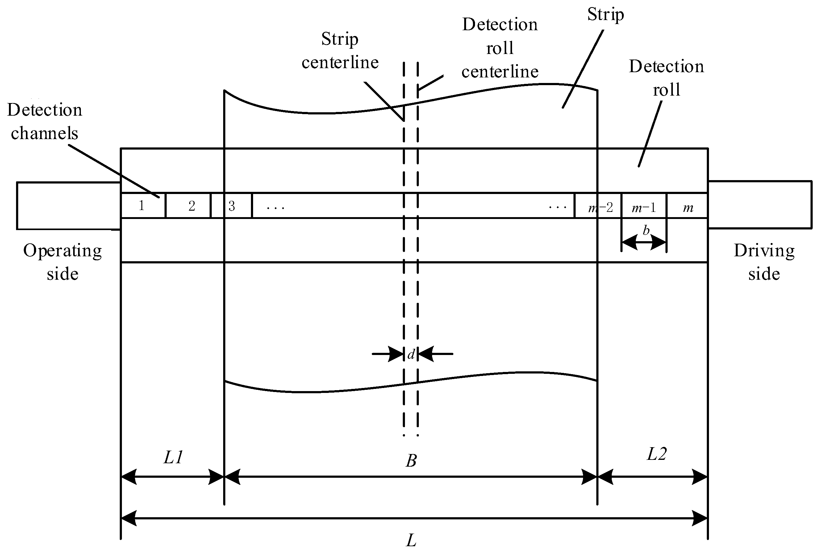
2.1. Determination of Valid Channels for Flatness Data

The flatness is often referred to as the wave shape. As shown in Figure 1, flatness is an indicator describing the uneven extension of the longitudinal fibers of the strip, which is intrinsically caused by the uneven distribution of residual internal stresses resulting from uneven calendering, cooling, and phase transformation at various points in the width direction of the strip during the production process.
As shown in the following equation, the relative length difference between different points in the width direction is taken to express flatness, also known as elongation difference.
ε x = Δ l / l
where εx is the elongation difference, the unit is IU; l is the post-rolling length of the reference point, generally taking the mid-point of the strip width as the reference point. Δl is the difference in the length after rolling at other points relative to the reference point.
The flatness detection roll provides discrete detection of the strip flatness through the individual detection channels. Due to the different specifications, the strip width differs from the detection rolls’ width, and the strip is subject to run-out during production, resulting in different uncovered areas on the left and right sides of the flatness data. Generally, when the detection channel covered by the strip edge is less than or equal to one third of the width of the inspection element, the channel flatness data are considered invalid. Otherwise, the channel flatness data are valid.
As shown in Figure 2, according to the structural characteristics of the detection roll, let the total number of inspection channels of the detection roll be m; the width of individual channels be b; the running deviation amount is d, specifying that the strip running deviation amount d towards the operating side is positive. Otherwise, it is negative; the distances from the operating side and the driving side on both sides of the strip are L1 and L2, respectively; the strip width is B; the inspection channels are numbered from the operation side to the drive side. L, L1, and L2 are as follows:
L = m × b
L 1 = L 2 ( B 2 + d )
L 2 = L 2 ( B 2 d )
The flatness data are read directly from the database and are deposited after the flatness meter has been processed, and the read strip flatness data are shown in Figure 3. The invalid flatness data value is 0. The strip flatness detection channels are numbered [1, 2,…, m] from left to right, and the strip flatness values are [y1, y2,…, ym] in that order. The valid channel determination formula on the operation side is: starting from i = 1, if yi = 0, then i + 1; otherwise, end, and the number of invalid channels on the left side is i + 1. The valid channels on the drive side are determined as follows: starting from j = m, if yj = 0, then j − 1; otherwise, end, and the number of invalid channels on the right side is mj.

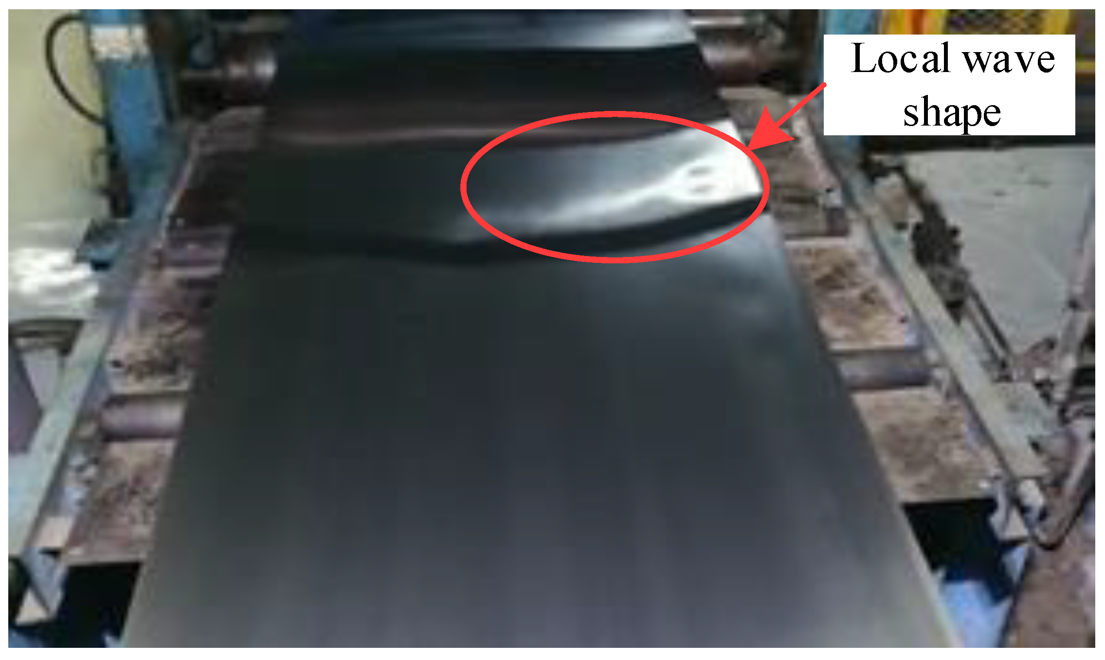
2.2. Extraction Algorithm of Local Wave Shapes

The local wave shape is represented by some form of buckling deformation of the strip, i.e., rolled to produce waves and warpage, as shown in Figure 4. The local wave shape extraction algorithm for wave shape is to identify tension stress distribution localized lower convex positions and extract them without affecting the overall wave shape pattern.

2.2.1. External Local Wave Shape Defect Recognition and Extraction

External local wave shape can be divided into external local wave shape defects on the operating and driving sides. The wave shape is in the form of a drop in the edge strip tension due to a significant edge elongation, which is determined and extracted. The treatment of external local wave shape defects on the operating side and the drive side is identical and is illustrated by the example of external local wave shape defects on the operating side.
It is assumed that a partial wave shape occurs at the position of channel 1 on the operating side. As shown in Figure 5, the number of valid channels from the operating side to the driving side is given as i = 1,2,…,m. The transverse coordinate corresponding to each channel is xi, and the valid flatness value corresponding to each effective channel is zi.
The steepness of the valid flatness data for the ith channel is as follows:
μ i = ( z i z i + 1 ) ( x i x i + 1 )
The width of each inspection channel of the flatness meter is the same and is b, b = x i + 1 x i . The above equation can be deformed as follows:
μ i = ( z i z i + 1 ) b
For the local shape wave of the ith channel, the position of the ith channel is assumed to be compensated by using the signals of adjacent channels to conduct interpolating compensation to the defect channel. Then, the local shape wave attached to ith channel is:
w i = z i z i
where w1, wm are external local waves, and the others are internal local waves.
Figure 5 shows that after the extraction of the local wave shape determination for the first channel, the overall flatness form is closer to the standard flatness defects, which can improve the overall flatness defect recognition accuracy.

2.2.2. Internal Local Wave Shapes Defect Recognition and Extraction

As shown in Figure 6, for the local shape wave of the ith channel, the position of the ith channel is assumed to be compensated by using the signals of adjacent channels to conduct interpolating compensation to the defect channel, as follows:
z i = { z i + 1 + b ( 2 μ i + 1 μ i + 2 ) , i = 1 z i 1 + z i + 1 2 + [ z i + 1 + b ( 2 μ i + 1 μ i + 2 ) ] 2 , i = 2 ( z i 1 + b μ i 2 ) + [ z i + 1 b ( 2 μ i + 1 μ i + 2 ) ] 2 , i = 3 [ z i 1 + b ( 2 μ i 2 μ i 3 ) ] + [ z i + 1 b ( 2 μ i + 1 μ i + 2 ) ] 2 , i ( 3 , m 2 ) [ z i 1 + b ( 2 μ i 2 μ i 3 ) ] + ( z i + 1 b μ i + 1 ) 2 , i = m 2 [ z i 1 + b ( 2 μ i 1 μ i 2 ) ] + z i 1 + z i + 1 2 2 , i = m 1 z i 1 + b ( 2 μ i 1 μ i 2 ) , i = m
Then, the local shape wave attached to ith channel is:
w i = z i z i
Figure 6 also shows that the overall flatness form is closer to the standard flatness defects after the extraction of local wave shape determination for channel i, which can improve the overall flatness defect recognition accuracy.

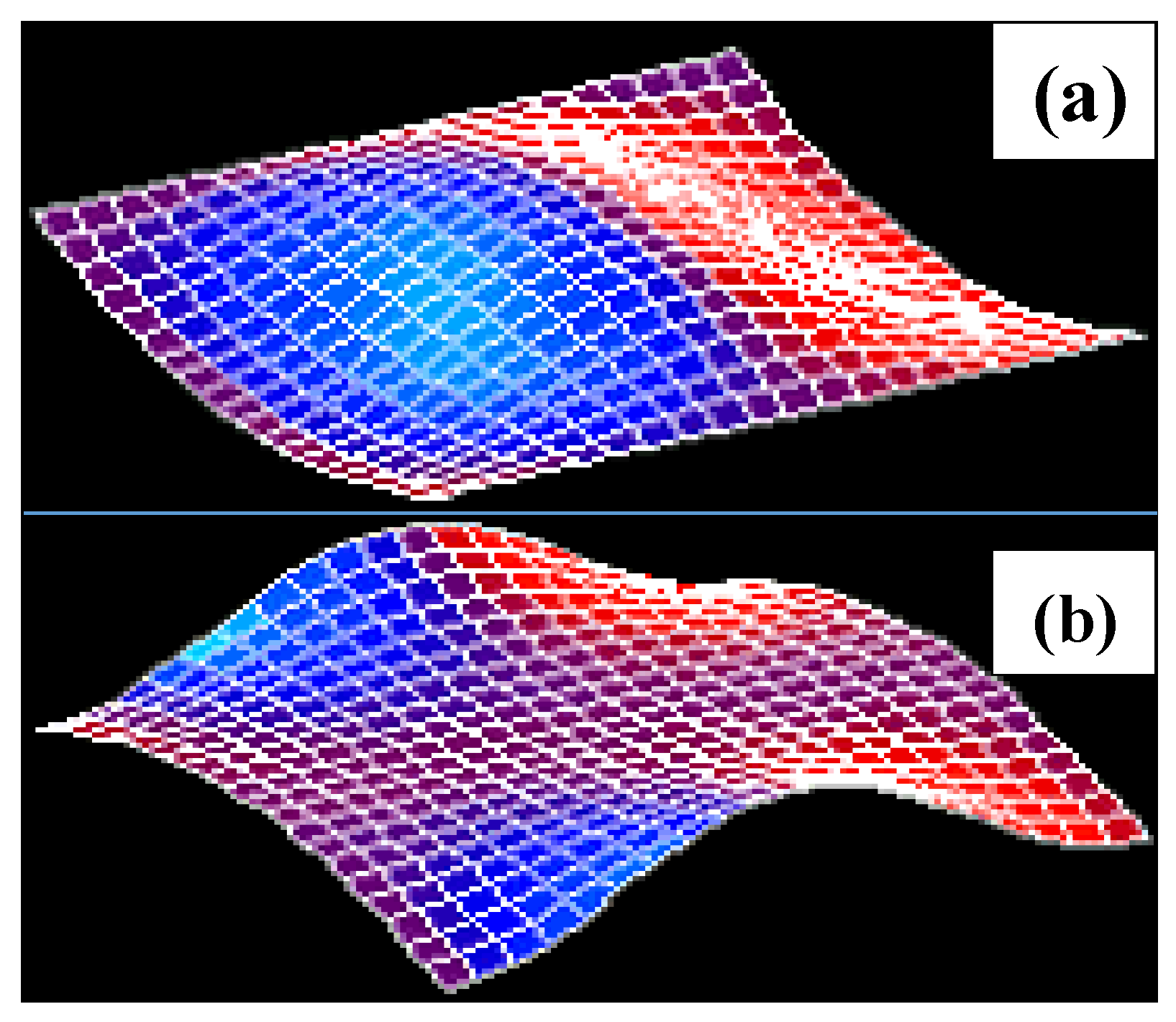
2.3. Overall Flatness Recognition Algorithm

The overall flatness defects are divided into primary, secondary, tertiary, and quaternary defects. The defect expressions of the basic flatness mode constructed using Legendre polynomials are as follows [17,18]:
Y 1 = p 1 ( y ) = y
Y 2 = p 1 ( y ) = y
Y 3 = p 2 ( y ) = 3 2 y 2 1 2
Y 4 = p 2 ( y ) = 3 2 y 2 + 1 2
Y 5 = p 3 ( y ) = 1 2 ( 5 y 3 3 y )
Y 6 = p 3 ( y ) = 1 2 ( 5 y 3 3 y )
Y 7 = p 4 ( x ) = 1 8 ( 35 y 4 30 y 2 + 3 )
Y 8 = p 4 ( x ) = 1 8 ( 35 y 4 30 y 2 + 3 )
Equations (9)–(16) are the standard normalized equations of the left wave, right wave, center waves, double-edge waves, left-one-third wave, right-one-third wave, quarter waves, and edge-center waves, respectively. Where y∈[−1, 1] is the normalized plate width coordinate, the origin is located in the center of the strip width.
The pattern recognition algorithm for overall flatness defect is based on the closeness principle. The current set of m measured flatness stress values is regarded as a new sample Y = [y1, y2,…,ym] to be identified, and the selected N types of basic flatness patterns are considered as N known standard samples Yk = [y1k, y2k,…, ymk], (k = 1,…N). To calculate the similarity of the current new sample Y to each standard sample, Yk, Y, and Yk are regarded as two m-dimensional space vectors, and the distance between the two vectors Dk can be worked out. In this paper, the cosine angle calculation formula with more obvious discrimination of multidimensional data is adopted:
D k = cos θ = Y · Y k | Y | | Y k | = i = 1 m y i y k i i = 1 m y i 2 i = 1 m y k i 2
In the flatness recognition, the eight basic flatness patterns selected have a symmetrical pattern of two and two inverses. From a mathematical point of view, if Yk and Yk + 1 are a standard sample of mutual inverse with Yk = −Yk + 1, Yk and Yk + 1 are linearly dependent. At the same time, as the output of the judgment result, two types of reciprocal flatness defects cannot exist simultaneously, so further processing is needed.
P P k = { D k D k + 1 , D k > D k + 1 0 , D k < D k + 1
Define µk to indicate the fuzz degree:
μ k = P P k i = 1 0.5 N | P P k | , k = 1 , 2 , 3 , , N 2
The positive and negative µk respectively represent two kinds of flatness defect modes opposite each other. The calculation diagram and flow chart of the above algorithm are shown in Figure 7.

2.4. Application of Flatness Recognition Algorithm for Local and Overall Flatness

The previous research extracts a set of flatness values (y1, y2, …, ym) from the local wave shape extraction method to obtain a group of local wave shape feature values. The local wave shape is extracted to obtain a smooth flatness array, which is used for the overall flatness defect pattern recognition, thus identifying local wave shape features and overall flatness features.
For the local shape wave extraction results, a set of local shape wave arrays {w1, w2,…, wm} can be obtained, and the maximum value in the array is used as the local shape wave feature of the measurement for quality judgment:
w = max [ w 1 , w 2 , , w m ]
For the whole flatness defect pattern recognition results, a group of similarities {μ1, μ2, μ3, μ4} can be obtained, which are primary flatness, secondary flatness, tertiary flatness, and quartic flatness, respectively. The similarity result cannot be directly used as the quality judgment value, so it must be further converted.
After the overall flatness recognition, the maximum flatness deviation ΔY of the flatness array is calculated:
Δ Y = max ( y 1 , y 2 , , y m ) min ( y 1 , y 2 , , y m )
By combining the maximum flatness deviation with flatness similarity, (Y1, Y2, Y3, Y4) are obtained as the overall flatness eigenvalue of each flatness pattern:
Y 1 = Δ Y μ 1 , Y 2 = Δ Y μ 2 , Y 3 = Δ Y μ 3 , Y 4 = Δ Y μ 4
According to the above calculation method, the calculation flow chart is shown in Figure 8.

3. Rules for Determining Cold-Rolled Strip Flatness Quality

In this section, the stress buckling calculation model of strip flatness with complex shape wave is used to establish the solution method of critical buckling strain difference under various representative shape wave conditions, and the criteria conditions of local shape wave and overall shape wave are formulated.
For the solution of the critical buckling elongation of flatness, firstly, the polynomials of the flatness stress and shape wave function under different buckling forms are constructed [19,20,21], as shown in Table 1.
The second-order variational equation of total potential energy, including bending strain energy and external force potential energy, is established as follows:
δ 2 ( ) = D 0 l b b [ ( 2 w y 2 ) 2 + ( 2 w x 2 ) 2 + 2 μ 2 w y 2 2 w x 2 + 2 ( 1 μ ) ( 2 w y x ) 2 ] d x d y + E h 0 1 b b [ ε f + ε a ( x ) ε p ( x ) ] ( w y ) 2 d x d y
where μ is poisson’s ratio; E is elasticity modulus; εf is average tensile stress; εa is post-tension during rolling; εp is rolling plastic elongation; h is strip thickness.
The condition that δ2(Π) has a stationary value is as follows:
[ δ 2 ( Π ) ] / r = 0
where r is the solution method of the lateral displacement constant in the waveform function, and the critical buckling elongation difference Δεp can be obtained.

4. Comprehensive Quality Evaluation of Cold-Rolled Strip Flatness

For the flatness, the flatness quality for each measurement must be expressed in a comprehensive index to directly evaluate the strip flatness condition. This section will evaluate the local and overall flatness characteristic values through a thorough evaluation.
The multi-objective decision evaluation problem is shown in Equation (25). fi(x) (i = 1, 2, …, m) is a continuous function of X.
max f ( x ) = ( f 1 ( x ) , f 2 ( x ) , , f n ( x ) ) s t . x X
The multiobjective evaluation method based on the closeness of the target introduces the concept of the membership function of the satisfaction of the objective function. This method can consider the requirements of the evaluator and perform relative quality evaluation by satisfying the closeness of the overall assessment and the ideal level.
Suppose the satisfaction of each goal μ(fi(x)) as Equation (21), where fi = (f1, f2,…, fn) and fi+ =( f1+, f2+,…, fn+) are ideal points and negative ideal points, respectively.
φ ( f i ( x ) ) = f i ( x ) f i f i + f i , i = 1 , 2 , , n
Suppose:
cos α = i = 1 n f i ( x ) f i + i = 1 n ( f i ( x ) ) 2 i = 1 n ( f i + ) 2 , cos β = i = 1 n f i ( x ) f i i = 1 n ( f i ( x ) ) 2 i = 1 n ( f i ) 2 , cos γ = i = 1 n f i + f i i = 1 n ( f i + ) 2 i = 1 n ( f i ) 2
Define goal closeness λ(x) as follows:
λ ( x ) = cos α cos γ cos α + cos β 2 cos γ
The flatness quality features are divided into a local wave shape and overall flatness characteristics. The flatness defect pattern recognition algorithm calculates: the internal local wave shape feature value w1, external local wave shape feature value w2, primary wave shape feature value Y1, the second wave shape characteristic value Y2, the third wave shape characteristic value Y3, and the fourth wave shape characteristic value Y4. The critical buckling strain difference Δε1, the external local wave shape characteristic value Δε2, the first wave shapes characteristic value ε1, the second wave shape characteristic value ε2, the third wave shape characteristic value ε3, and the eigenvalue of the fourth wave shape ε4 are calculated by the method of rulemaking for determining the flatness quality.
The flatness mass vector f = (w1, w2, Y1, Y2, Y3, Y4) is constructed. The ideal target of flatness is the target flatness f+ = (0, 0, 0, 10, 0, 0) with certain quadratic convexity. Flatness negative ideal target is f− = (ε1, ε2, ε3, ε4, ε5, ε5, ε6). According to Equations (27)–(29), the flatness comprehensive quality λ can be calculated.
In order to verify the practicality of the above determination method, use the field data of a cold rolling single stand six-high mill for verification. Field data include thickness, strip width, tension, and flatness data. Based on the strip specification, the critical buckling strain difference is calculated in real time for the strip’s overall flatness and localized wave shape, as shown in Table 2.
The critical buckling strain difference of the overall and local flatness defects is based on the calculated critical buckling strain differences for the center, double-side, internal local, and external waves. The critical buckling strain difference of the double-side wave shape is used for single-side, double-side, and edge-center waves, and the critical buckling strain difference of the center wave shape is used for center, one-third, and quarter waves. The quality pass thresholds assigned to all flatness patterns for the eight samples above are shown in Table 3.
According to the process of flatness quality determination, local shape wave extraction and overall flatness defect identification are carried out for the eight test samples above. According to the comprehensive quality calculation method, the characteristic value of various flatness defects is calculated as a comprehensive quality evaluation value. The range of comprehensive quality evaluation values is [0, 1]. When the value is 1, it means that it is entirely close to the ideal flatness, and when the value is 0, it is utterly close to the negative ideal flatness. In this paper, the quality rating of the above eight samples is demonstrated, in which [0.7, 1], (0.5, 0.7), and [0, 0.5] are taken as grade A, grade B, and grade C, respectively. Each sample’s eigenvalues for each flatness defect pattern, the comprehensive quality evaluation value, and the grading results are shown in Table 4.

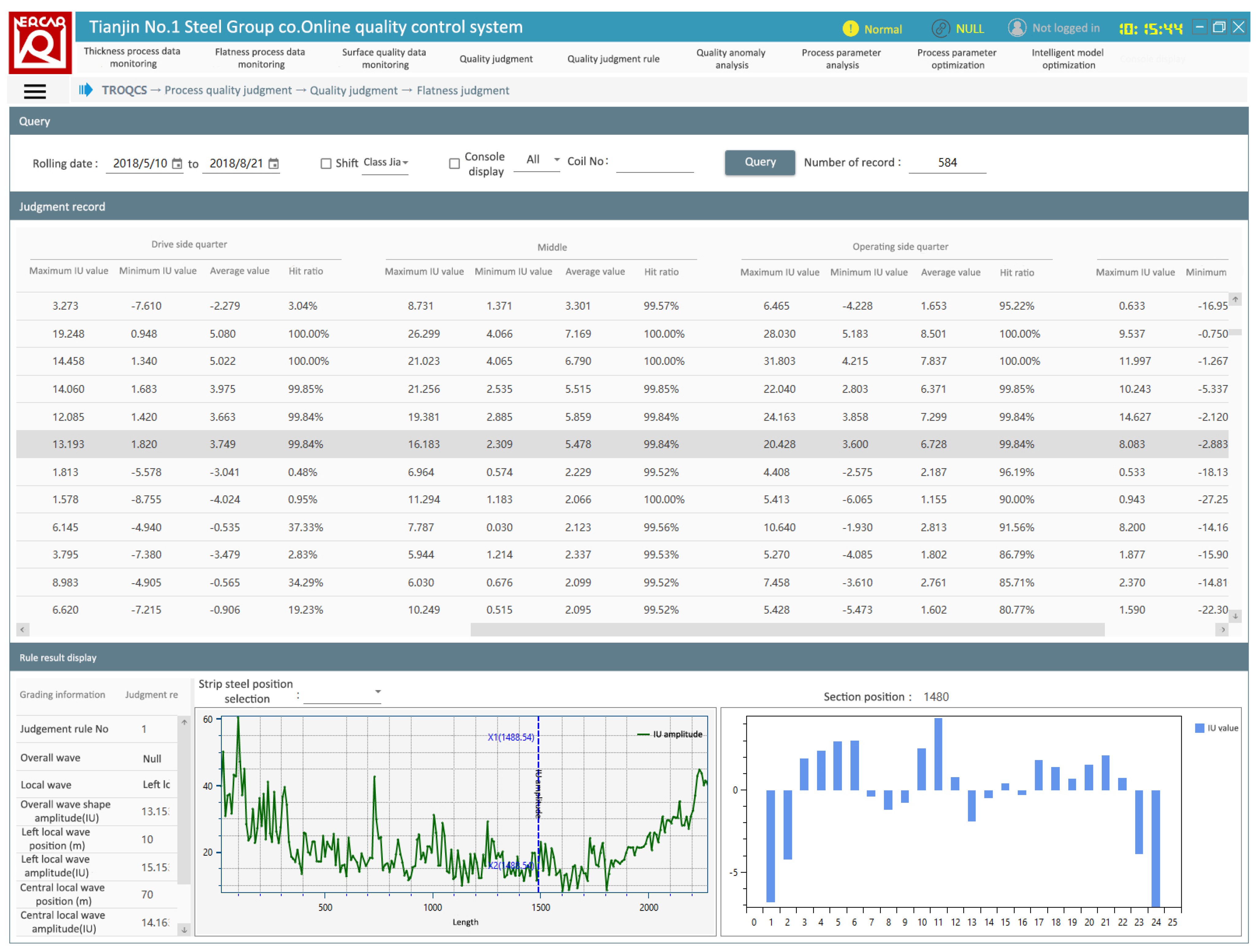
5. Application of Flatness Quality Determination in Cold Rolling

By using C # computer programming language (Microsoft Visual Studio 2012), the flatness quality judgment system of cold rolled strip is designed and implemented. The flatness online judgment visualization display, data reading, pattern recognition, quality judgment, etc., have been completed. The operation interface is shown in Figure 9. In the judgment record box, the basic information of the strip, the quality status and level of flatness judgment, and the flatness control situation of the head, middle, and ending sections of the strip are included. In the judgment rule display box, the left side is the judgment rule and the judgment result and the right side is the flatness status of the strip at the mouse click position and the average deviation result of the flatness meter along the whole strip length.
The system functions are running stably after a year of online trial operation. Applying this cold rolling quality control platform has brought apparent improvement effects for the enterprise in the following aspects.
  • The application of this system has improved the level of process quality data management, changed the original situation of quality data being stored piecemeal in multiple systems, and stored process quality data in the same platform after cleaning, sorting, and organizing, making it easy for users to query, download, and statistically analyze the data.
  • The input of the quality judgment function significantly shortens the quality judgment time. It improves the production efficiency while avoiding the arbitrariness of manual judgment, improving the accuracy of quality judgment and realizing the decision guidance for the production post-process.

6. Conclusions

The quality determination system researched and designed in this paper provides powerful support for product quality determination of thin strip products containing local and overall flatness, improves the reference for optimizing process parameters, and has high practical value. The details are as follows:
  • A local wave extraction algorithm and a similar distance formula for the overall flatness pattern recognition algorithm are designed. For the recognition accuracy of local wave shape and the recognition accuracy of overall flatness defects in strip quality determination, a smooth flatness curve based on local wave shape extraction is proposed for overall flatness defect recognition. Meanwhile, the distance evaluation formula in the fuzzy classification algorithm is optimized, and the application method of cosine similarity is proposed.
  • The strip stress buckling models for local and overall wave shapes were investigated by introducing the small displacement buckling theory for thin strips. The critical buckling stresses for overall and local wave shape under given conditions were calculated as the corresponding quality determination thresholds. The quality determination model of flatness containing both local and overall wave shapes was validated using field flatness data.
  • A comprehensive quality determination model of the flatness was established. By using the multiobjective integrated evaluation method, we evaluated the local wave shape quality and the overall flatness quality of the strip, and the strip flatness quality was further rated using the evaluation value.
  • Through C# computer programming, the determination process—such as visual display of online determination of flatness, storage and query of determination results, pattern recognition algorithm, and calculation of comprehensive quality determination— is completed, which provides a reference for the field application of cold-rolled strip flatness quality determination system.

Author Contributions

Q.W. analyzed the simulation data and completed the draft; J.L. helped to write and debug all algorithms; X.W. and Q.Y. instructed the revision of the draft; Z.W. helped to draw the diagrams and tables. All authors have read and agreed to the published version of the manuscript.

Funding

This research was funded by the National Natural Science Foundation of China (Grant No. 51975043); the National Key Research and Development Plan (Grant No. 2020YFB1713600); the Fundamental Research Funds for the Central Universities (Grant No. FRF-TP-20-105A1); and the China Postdoctoral Science Foundation (Grant No. 2021M690352).

Institutional Review Board Statement

Not applicable.

Informed Consent Statement

Not applicable.

Data Availability Statement

Data sharing not applicable. No new data were created or analyzed in this study. Data sharing is not applicable to this article.

Conflicts of Interest

The founding sponsors had no role in the design of the study; in the collection, analyses, or interpretation of data; in the writing of the manuscript; or in the decision to publish the results.

References

  1. Abdelkhalek, S.; Zahrouni, H.; Legrand, N.; Potier-Ferry, M. Post-buckling modeling for strips under tension and residual stresses using asymptotic numerical method. Int. J. Mech. Sci. 2015, 104, 126–137. [Google Scholar] [CrossRef]
  2. Kpogan, K.; Zahrouni, H.; Potier-Ferry, M.; Dhia, H.B. Buckling of rolled thin sheets under residual stresses by ANM and Arlequin method. Int. J. Mater. Form. 2017, 10, 389–404. [Google Scholar] [CrossRef] [Green Version]
  3. Bao, R.R.; Zhang, J.; Li, H.B.; Jia, S.H.; Liu, H.J.; Xiao, S. Flatness pattern recognition of ultra-wide tandem cold rolling mill. Chin. J. Eng. 2015, 37, 6–11. [Google Scholar]
  4. Zhang, Q.D.; Chen, X.L.; Xu, J.W. Method of Flatness Defect Pattern Recognition. Iron Steel 1996, 31, 57–60. [Google Scholar]
  5. Dai, J.B.; Wu, W.B.; Zhang, Q.D.; Wang, J.F.; Wang, H. Recognition and Evaluation System for Strip Flatness on 2030mm Cold Tandem Mills. J. Univ. Sci. Technol. Beijing 2003, 25, 572. [Google Scholar]
  6. He, H.T.; Li, Y. A new flatness pattern recognition model based on cerebellar model articulation controllers network. J. Iron Steel Res. Int. 2008, 15, 32–36. [Google Scholar] [CrossRef]
  7. Song, J.J.; Shao, K.Y.; Chi, D.X.; Hua, J.X.; Zhang, Q. Application of wavelet analysis in recognizing the defects of plate Form in rolling process. Control. Decis. 2002, 17, 69–72. [Google Scholar]
  8. Zhang, X.L.; Zhang, S.Y.; Tang, G.Z.; Zhao, W.B. A novel method for flatness pattern recognition via least squares support vector regression. J. Iron Steel Res. Int. 2012, 19, 25–30. [Google Scholar] [CrossRef]
  9. He, H.T.; Li, N. The improved RBF Approach to Flatness Pattern Recognition Based on SVM. J. Autom. Instrum. 2007, 28, 1–4. [Google Scholar]
  10. Zhang, C.; Tan, J.P. Strip flatness pattern recognition based on genetic algorithms-back propagation model. J. Cent. South Univ. 2006, 37, 294–299. [Google Scholar]
  11. Li, X.G.; Fang, Y.M.; Liu, L. Kernel extreme learning machine for flatness pattern recognition in cold rolling mill based on particle swarm optimization. J. Braz. Soc. Mech. Sci. Eng. 2020, 42, 270. [Google Scholar] [CrossRef]
  12. Yang, J.; Xu, Q. Quantum ant colony optimizing theory and its application in fuzzy pattern recognition method of flatness. Int. Conf. Comput. Sci. Technol. 2017, 12508, 210–216. [Google Scholar] [CrossRef] [Green Version]
  13. Wang, Y.; Hu, H.Q. The shape recognition in cold strip rolling based on SVM. Appl. Mech. Mater. 2013, 427, 1687–1690. [Google Scholar] [CrossRef]
  14. Zhang, X.L.; Zhao, L.; Zang, J.Y.; Fan, H.M. Visualization of flatness pattern recognition based on T-S cloud inference network. J. Cent. South Univ. 2015, 22, 560–566. [Google Scholar] [CrossRef]
  15. Zhang, X.L.; Zhang, Z.Q. A novel method of optimal designing DHNN and applied to flatness pattern recognition. CAAI Trans. Intell. Syst. 2008, 3, 250–253. [Google Scholar]
  16. Wang, Y.Q.; Yin, G.F.; Sun, X.G. Research for pattern recognition of shape signal method. Chin. J. Mech. Eng. 2003, 39, 91–94. [Google Scholar] [CrossRef]
  17. Zhang, X.L.; Cheng, L.; Hao, S.; Gao, W.Y.; Lai, Y.J. The new method of flatness pattern recognition based on GA–RBF–ARX and comparative research. Nonlinear Dyn. 2016, 83, 3. [Google Scholar] [CrossRef]
  18. Jia, C.Y.; Shan, X.Y.; Liu, H.M.; Niu, Z.P. Fuzzy Neural Model for Flatness Pattern Recognition. J. Iron Steel Res. Int. 2008, 15, 33–38. [Google Scholar] [CrossRef]
  19. Yang, Q.; Chen, X.L. Target Model of the Automatic Shape Control on Cold Strip Mill. J. Univ. Sci. Technol. Beijing 2003, 27, 142–145. [Google Scholar]
  20. Peng, Y.; Liu, H.M. Pattern Recognition Method Progress of Measured Signals of Shape in Cold Rolling. J. Yanshan Univ. 2003, 27, 142–145. [Google Scholar]
  21. Yang, Q.; Chen, X.L. The Deforming Route of Buckled Waves of Rolled Strip. J. Univ. Sci. Technol. Beijing 1994, 16, 53–57. [Google Scholar] [CrossRef]
Figure 1. Common symmetrical flatness defects. (a) Center waves; (b) double-sided waves.
Metals 12 01977 g001
Figure 2. The diagram to determine the number of valid channels for the flatness detection roll.
Metals 12 01977 g002
Figure 3. Diagram of the flatness data reading results.
Metals 12 01977 g003
Figure 4. Local wave shapes on site.
Metals 12 01977 g004
Figure 5. Principle of the external local wave shape defect recognition and extraction.
Metals 12 01977 g005
Figure 6. Principle of the internal local wave shape defect recognition and extraction.
Metals 12 01977 g006
Figure 7. The flow chart of flatness pattern recognition calculation. (PPk is is the result of calculating two mutually inverted flatness defects according to Equation (19), k = 1,2,3,4).
Metals 12 01977 g007
Figure 8. The flow chart of flatness eigenvalues.
Metals 12 01977 g008
Figure 9. The interface of the flatness quality evaluation system.
Metals 12 01977 g009
Table 1. The flatness stress and wave function of various bucking modes.
Buckling FormFunction NameFormula
External local wave bucklingFlatness stress ε p ( x ) = Δ ε p [ ( x b + b w b w ) n E b w ( n E + 1 ) b ]
shape wave function { w ( x , y ) = r ( x b + b w b w ) n w sin ( π y / l ) , ( b b w x b ) w ( x , y ) = 0 , ( 0 < x < b b w )
Internal local wave bucklingFlatness stress ε p ( x ) = Δ ε p [ e 0 ( 1 b w b ) + e 2 ( ( x b w ) 2 b w 3 b ) + e 4 ( ( x b w ) 4 b w 5 b ) + e 6 ( ( x b w ) 6 b w 7 b ) + e 8 ( ( x b w ) 8 b w 9 b ) ]
shape wave function { w ( x , y ) = r [ r 0 + r 2 ( x b w ) 2 + r 4 ( x b w ) 4 + r 6 ( x b w ) 6 + r 8 ( x b w ) 8 ] sin ( π y l ) , ( b w x b w ) w ( x , y ) = 0 , ( b < x < b w , b w < x < b )
Overall wave bucklingFlatness stress ε p ( x ) = Δ ε p [ e 0 ( 1 b w b ) + e 2 ( ( x b w ) 2 b w 3 b ) + e 4 ( ( x b w ) 4 b w 5 b ) ]
shape wave function w ( x , y ) = r [ r 0 + r 2 ( x b w ) 2 + r 4 ( x b w ) 4 ] sin ( π y l ) , ( b x b )
Note: b is the strip half-width; bw is the buckling defect size; nw, n0n8 are the deflection function coefficients; ne, e0e8 are the stress function coefficients.
Table 2. Cold rolling site sample data.
NumberSteel GradeThickness
/mm
Width
/mm
Tension
/Mpa
Critical Buckling Strain Difference
Center WavesDouble-Sided WavesInternal Local WavesExternal Local Waves
1SPCC-1B0.2890910.932.3728.6115.0717.94
2SPCC-1B0.2890910.230.2926.7814.116.78
3SPCC-1B0.3290410.932.3728.6115.0917.95
4SPCC-1B0.3290410.932.3728.6115.0917.95
5SPCC-1B0.6690410.932.3828.6215.1617.99
6SPCC-1B0.6690410.932.3828.6215.1617.99
7SPCC-1B0.3790410.330.5927.0414.2716.97
8SPCC-1B0.3790410.129.9926.5113.9916.64
Table 3. Quality conformity thresholds for all flatness defects patterns.
NumberInternal Local WavesExternal Local WavesSingle-Edge WavesCenter WavesDouble-Edge WavesOne-Third WavesQuarter WavesEdge-Center Waves
115.0717.9428.6132.3728.6132.3732.3728.61
214.116.7826.7830.2926.7830.2930.2926.78
315.0917.9528.6132.3728.6132.3732.3728.61
415.0917.9528.6132.3728.6132.3732.3728.61
515.1617.9928.6232.3828.6232.3832.3828.62
615.1617.9928.6232.3828.6232.3832.3828.62
714.2716.9727.0430.5927.0430.5930.5927.04
813.9916.6426.5129.9926.5129.9929.9926.51
Table 4. Results of flatness quality comprehensive evaluation.
NumberSteel Gradew1w2Y1Y2Y3Y4λGrade
1SPCC-1B29.320.002.1152.2825.381.440.528B
2SPCC-1B21.110.003.6835.304.4713.730.523B
3SPCC-1B20.010.005.0049.982.449.380.576B
4SPCC-1B20.110.004.9438.305.906.580.548B
5SPCC-1B17.970.003.0630.362.789.810.543B
6SPCC-1B17.670.003.9827.9413.0116.160.456C
7SPCC-1B33.270.006.3557.886.884.360.566B
8SPCC-1B23.430.006.0445.3715.685.300.528B
Publisher’s Note: MDPI stays neutral with regard to jurisdictional claims in published maps and institutional affiliations.

