Abstract
The improvement in mixing conditions in a vacuum refining unit plays an important role in enhancing the purity and decarburization of molten steel. Mixing time is an important index to evaluate the operation efficiency of a metallurgical reactor. However, in water models, the effect of salt tracer dosages on the measured mixing time in a vacuum reactor is not clear. In this study, a water model of a Single Snorkel Refining Furnace (SSRF) was established to study the effect of salt solution tracer dosages on the mixing time of monitor points. The experimental results show that, in some areas at the top of the ladle, the mixing time decreases first and then increases when increasing the tracer dosage. Numerical simulation results show that, when the tracer dosage increases, the tracer flows downwards at a higher pace from the vacuum chamber to the bottom of the ladle. This may compensate for the injection time interval of large dosage cases. However, the mass fraction of the KCl tracer at the right side of the bottom is the highest, which indicates that there may be a dead zone. For the dimensionless concentration time curves and a 99% mixing time, at the top of the vacuum chamber, the curve shifts to the right side and the mixing time decreases gradually with the increase in tracer dosage. At the bottom of the ladle, with the increase in tracer dosage, the peak value of the dimensionless concentration time curve is increased slightly. The mixing time of the bottom of the ladle decreases significantly with the increase in tracer dosage. However, in the dead zone, the mixing time will increase when the tracer dosage is large. At the top of the ladle, the effect of the tracer dosage is not obvious. The mixing time of the top of the ladle decreases first and then increases when increasing the tracer dosage. In addition, the mixing time of the top of the ladle is the shortest, which means that sampling at the top of the ladle in industrial production cannot represent the entire mixing state in the ladle.
1. Introduction
The Single Snorkel Refining Furnace (SSRF) is a revolutionary vacuum refining unit that can satisfy the higher treatment efficiency of molten steel. It was developed based on a modification of Ruhrstahl-Heraeus (RH) in the 1970s [1]. It is composed of a vacuum chamber, a single snorkel and a ladle with an eccentric blowing nozzle at the bottom. Similarly, a novel vacuum degassing process consisting of a large immersion snorkel and a bottom bubbling ladle called the Revolutionary Degassing Activator (REDA), which has similar furnace structure and metallurgical principle to SSRF, was developed by Nippon Steel Corporation Yawata Works in 1990s [1,2]. It has been applied to produce ULC steel and stainless steel.
As the flow of molten steel in the refining process has an important influence on inclusion, removal, decarburization, desulfurization, alloy mixing and steel scrap melting [3,4,5,6,7,8,9], physical modeling and numerical simulations have been established to investigate the flow and mixing phenomena of molten steel in ladle refining [10,11,12,13,14,15,16,17,18,19], RH [20,21,22,23,24,25,26,27,28,29,30,31,32,33] and SSRF [34,35,36,37]. Many researchers have investigated the effect of diameter [20,34], number [21], shape [22,35] and immersion depth [36] of the snorkel, as well as arrangement [34] and number [30] of nozzles, gas flow rate [20,21,23,24,31,32], combined bottom blowing [20,33] and pressure of the vacuum chamber [23,25,26] on mixing time and the circulation rate in SSRF and RH.
Mixing degree or mixing time is an important index to evaluate the operation efficiency of a metallurgical reactor. Tracer technology [38] and tracers have been widely used to track the fluid flow and to measure the mixing time. In the study of the water model, salt solution tracers are usually added and the changes in electrical signals at specific monitor points are measured to calculate the mixing time. However, the physical property of the salt solution tracer is not identical to the main fluid, namely water. Note that the density of saturated salt solution for example KCl solution is 1163.2 kg/m3 [39], which is 16% heavier than that of water. This difference may influence the fluid flow and measured data in the experiments. Table 1 shows the use of salt solution tracers, such as the KCl or NaCl solution injection in the SSRF or RH water model, used by many researchers. Due to the great difference between the water volume and the dosage of salt solution tracers in the water model, the dimensionless ratio of the tracer dosage to the water volume is evaluated in this study. It is found that the dosage of the tracer in each liter of water is greatly different, which range from 0.027 mL [40] to 1.265 mL [41]. There is a 45 times difference between the two cases. It is not clear whether the salt tracer dosage will influence the experimental results in the SSRF water model. At the same time, there are a few reports on this topic.

Table 1.
Summary of tracer injection in the water model of RH and SSRF.
Chen et al. [44] showed that, for continuous casting tundish, the residence time distribution (RTD) curve of the salt solution tracer is deviated to the left side of the calculated curve, this deviation is even larger with an increasing tracer dosage from 50 to 250 mL. Chen et al. [45,46] further studied the flow behavior in a continuous casting tundish by numerical simulation, and found that the upward flow of a tracer will, sooner or later (depending on the dosage), sink to the bottom due to the higher density of the tracer compared to that of the water. Ding et al. [47,48] conducted numerical simulation on the metallurgical tundish and found that, with the increase in the mass concentration and the volume of the tracer, the shape of the RTD curve changes from single flat peak to single sharp peak and then to double peaks. For gas-stirred ladle systems, Chen et al. [49] showed that the obtained mixing time decreased as the tracer dosage increased. By using numerical models, Zhang et al. [16] found that KCl solution tracer could complete the mixing process much faster than the pure water tracer (density is identical to water phase). Gómez et al. [50] found that, for the ladle water model, the tracer concentration has also been found to have an effect on mixing time, however this effect is obvious only at low gas flow rates. At high gas flow rates, differences in tracer concentration have no obvious effect on mixing time. However, the influence of salt solution tracer on the flow and transport process of tracer in SSRF water model is thus far not clear.
In addition, Computational Fluid Dynamics (CFD) methods have been widely used to study flow behavior [51,52,53,54,55,56,57,58,59,60], mixing phenomenon [51,52,53] and decarburization mechanism [54,55,56] in SSRF or REDA. However, in CFD study, the density of the tracer is often considered to be the same as liquid (water), and the transport of salt solution tracer cannot be accurately simulated. The possible effects of the salt solution tracer density and dosage on the mixing process are generally ignored. Therefore, in this study, a CFD model, combined with a water model, were used to study the transport process of the salt solution tracer in the water model of SSRF and the effect of tracer dosages on fluid flow and transport process of tracer. The transport process of the salt tracer in the water model will be clarified, which can provide hints for the water model experiment and industrial SSRF production.
2. Model Descriptions
2.1. Physical Modeling
SSRF water model experimental installation is shown in Figure 1. The geometrical parameters of an industrial 130 t SSRF and corresponding water model are listed in Table 2. The water model was scaled down by a factor of 1/5 according to the Froude number similarity.
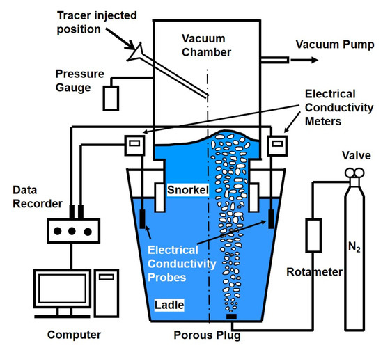
Figure 1.
Schematic diagram of experimental installation.
Table 2.
Parameters of the water model and industrial geometry.
For physical modeling, the stimulus–response technique was used to study the salt solution tracer transport process in the water model of SSRF. After the steady state of fluid flow was obtained, the KCl solution tracer was injected by a funnel from the vacuum chamber. The electrical conductivity was measured by conductivity probes, which are located at different positions of the ladle. The electrical conductivity data were collected by the data recorder. When the conductivity curve is stable within a certain range, for example ±1% or ±5% as the dotted line shown in Figure 2, it is considered that the system has been completely mixed, and the time is defined as the mixing time from a chemical or metallurgical reaction engineering perspective. The determination of mixing time is schematically shown in Figure 2.
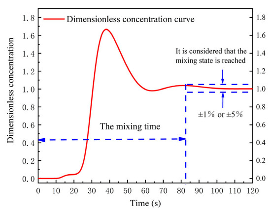
Figure 2.
Schematic diagram of dimensionless concentration curve (the dotted lines are fluctutaion range and mixing time).
2.2. Studied Cases
Based on the statistical results of tracer dosages (Table 1) and water volume (149 L) in this study, seven tracer dosages were studied, i.e., 20 mL, 40 mL, 60 mL, 80 mL, 100 mL, 150 mL, and 250 mL KCl saturated solution, as shown in Table 3. The difference between the maximum and the minimum is 12.5 times. The dimensionless tracer dosage range, which covers the main range in Table 1, is 0.1342 mL to 1.6779 mL in each liter of water. In the water model experiment, the dosage of KCl saturated solution was 40 mL, 60 mL, 80 mL, 100 mL and 150 mL. In the numerical simulation, in order to further study the influence of tracer dosage on the transport process of tracers, in addition to the above five cases, two small and large dosages of KCl solution cases were also studied, which were 20 mL and 250 mL, respectively.
Table 3.
Dosages of the KCl solution tracer.
In addition, because the density of the KCl solution is higher than that of water, the influence caused by the density difference between the tracer and water cannot be eliminated in the water model experiments. Therefore, in the numerical simulation, the other two kinds of tracers, including pure water (without density effect) and passive scalar (without physical property), are also studied.
For the numerical simulation, after predicting the steady flow field of SSRF water model, the multicomponent fluid model and passive scalar transport model were used to simulate the transport process of the tracer in the water model. Specific model descriptions are presented in Section 2.3.
2.3. Numerical Simulation
2.3.1. Model Assumptions
The Euler-Euler method was used to numerically simulate the gas-liquid multiphase flow in the SSRF water model. The following assumptions were made: (1) Both gas and liquid are Newtonian fluids, viscous and incompressible. (2) The top free surface of the ladle and the free surface of the vacuum chamber are assumed to be smooth and frictionless. (3) The bubbles are spherical, and their sizes are assumed to be a constant. The coalescence, collision and breakup of the bubbles are ignored. (4) The flow is isothermal. (5) The solid wall is a non-slip boundary; the wall function is applied near the wall.
2.3.2. Euler-Euler Model
The Euler-Euler model solves a set of conservation equations for each Euler phase appearing in the simulation. The pressure is assumed to be the same in all phases. The volume fraction gives the share of the flow domain that each phase occupies. Each phase has its own velocity and physical properties. The main equations are summarized as follows.
Volume fraction equation: The proportion of each phase in the fluid region is given by its volume fraction. The volume of phase i is given by the following formula.
where α is the volume fraction of the phase, and i represents the gas phase or liquid phase. The volume fraction of each Euler phase must satisfy the following requirement.
where n is the total number of phases.
Continuity equation: The mass conservation of phase i is given by the following equation.
where ρ is the density of the phase and u is the average velocity of the phase.
Momentum equation: The momentum conservation of phase i is given by the following equations.
where is the gravity acceleration vector, P is the pressure shared by gas-liquid two phases, is the interphase momentum transfer per unit volume, and μieff is effective viscosity, which is composed of phase dynamic viscosity μi and phase turbulent viscosity μt,i.
Interphase Momentum Transfer: The momentum transfer term consists of contributions from the drag, virtual mass, lift, and turbulent dispersion forces.
where the subscripts l and g represent the liquid phase and gas phase, respectively, and FD, FVM, FL and FTD on the right side of the equation represent drag force, virtual mass force, lift force and turbulent dissipation force, respectively.
Drag Force: The drag force model calculates the force on a particle in the dispersed phase due to its velocity relative to the continuous phase. The drag force is modeled as a linear multiplier of the relative velocity between the two phases. The force acting on the gas phase due to the drag of the liquid phase is implemented as follows.
where AD is the linear drag coefficient and ur is the relative velocity between the gas phase and the liquid phase. The linear drag coefficient AD is related to the standard engineering definition of the particle drag coefficient, and the formula is given as follows.
where dg is the bubble diameter, which is considered to be a constant in the simulation. It can be calculated using the following formula, which was proposed by Sano et al. [61]. Where σ is the surface tension, the value of σ is 0.072 (N∙m−1). is the initial velocity of bubbles at the nozzle, which is related to the gas flow rate and the diameter of the nozzle.
In Equation (9), CD is drag coefficient. In the formula proposed by Schiller-Naumann [62], when Reg > 1000, the drag coefficient is 0.44, so it is 0.44 in this study. Reg is the bubble Reynolds number as follows.
Lift Force: When the continuous phase flow field is uneven or rotating, the discrete phase will be lifted perpendicular to the relative velocity. The calculation formula is as follows.
where CL is the lift coefficient. In this study, the lift coefficient 0.5 proposed by Auton et al. [63] is used.
Virtual Mass Force: The virtual mass force model explains the additional resistance that particles experience when accelerating through the fluid. When the density of the particles is equivalent to that of the surrounding fluid or much smaller than that of the surrounding fluid, this resistance will be large. The virtual mass force acting on the gas phase by the acceleration of the gas phase relative to liquid phase can be expressed by the following equation.
where CVM is the virtual mass coefficient, and ag and al are the acceleration rate of gas phase and liquid phase, respectively.
Turbulent Dispersion Force: Turbulent dispersion force model that accounts for the interaction between the dispersed phase and the surrounding turbulent eddies. The effect of turbulence in the redistribution of nonuniformities in phase concentration is modeled by an additional turbulent dispersion force in the phase momentum equations. The term has the following form.
where uTD is a relative drift velocity defined by the volume fraction weighting, and DTD is a tensor diffusion coefficient.
2.3.3. Turbulence Model
The Realizable Two-Layer k-ε model [64,65] was used in this study. The specific equations are as follows.
where Pk,i and Pε,i are production terms of phase i, which depends on the k-ε model. σk, σε, Cε1 and Cε2 are model coefficients, and their values are 1, 1.2, 1.44 and 1.9, respectively. For the two-layer models, the dissipation rate ε near the wall is simply prescribed as follows.
where lε,i is a length scale function of phase i that is calculated according to Wolfstein [66].
where d2 is the distance to the wall, Cμ is a model coefficient of 0.09, Red2 is the wall-distance Reynolds number, and υi is the kinematic viscosity of phase i.
2.3.4. Tracer Transport Model
The tracer transport model includes the multicomponent fluid model and passive scalar transport model. The multicomponent fluid model is used to predict the transport process of tracer (KCl solution or pure water) in water. The model is described as follows.
where WT is the mass fraction of water and tracer (KCl solution or pure water), respectively. When tracers are injected into the top inlet of the water model, WT = 1. When the injection of tracers is stopped, WT = 0. The injection time interval can be derived from the tracer volume divided by the cross section area of the tracer inlet and inlet velocity. For example, 0.4 s for 20 mL KCl solution tracer case. The effective diffusion coefficient Deff is the sum of the molecular diffusion coefficient and turbulent diffusion coefficient, as follows.
where Dl is the molecular diffusion coefficient of liquid phase and Dt,l is the turbulent diffusion coefficient, which is expressed by the following formula.
Sct,l is the turbulence Schmidt number, which was set as 0.9 in the model. υt,l is the turbulence kinematic viscosity.
The density of the mixing fluid in all the continuity, momentum, and turbulence equations are calculated as follows.
where ρw and ρT are the density of water and tracer, respectively.
Passive scalar transport model is used to predict the transport process of passive scalar in this study. Passive scalar is a virtual tracer, which has no physical properties and only passively transports with the flow of water. The description is as follows.
where WS is the mass fraction of the passive scalar.
2.4. Mesh, Boundary Conditions and Materials Properties
2.4.1. Mesh
The 3D geometric model of the SSRF water model was established. A polyhedral mesh was used in the simulation, as shown in Figure 3. A mesh with 714,383 grids was used in the present study.
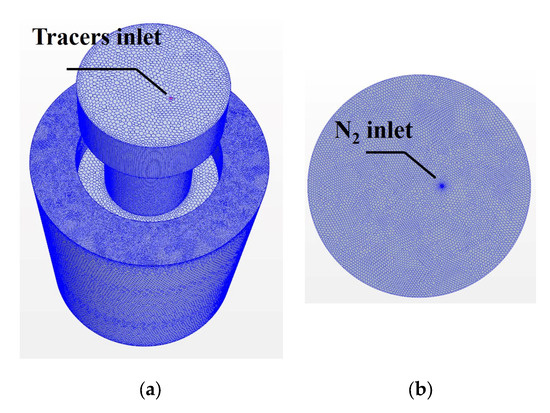
Figure 3.
Mesh of SSRF: (a) Front view and (b) the bottom of the ladle.
2.4.2. Boundary Conditions
The walls of the ladle, snorkel and vacuum chamber were set as a non-slip boundary condition. The standard wall function was applied to the near-wall region. In addition, a wall boundary condition was used for the top surfaces of the liquid phase both at the ladle and the vacuum chamber. However, the bubbles are allowed to escape from the top surfaces. The inlet velocity of the nozzle was calculated according to the total gas flow rate. The volume fraction of water was zero at the nozzle. The turbulent kinetic energy and its dissipation rate at the entrance were calculated by the method proposed by Ilegbusi et al. [67], as follows.
where rn is the radius of the nozzle.
2.4.3. Materials Properties
The density of KCl solution is 1163.2 kg/m3 [39] and the density of the pure water is 997.561 kg/m3 [39]. The density of KCl solution is higher than that of pure water. Passive scalar is a virtual tracer without physical properties. In addition, other properties of physical tracers are also considered in this study. The diffusion coefficient of KCl solution is 1.994 × 10⁻⁹ m2/s [45,68], and that of pure water is 2.216 × 10⁻⁹ m2/s [69]. The dynamic viscosity of KCl solution tracer is 1.04 × 10⁻³ Pa⦁s [39], and that of pure water is 8.8871 × 10⁻⁴ Pa⦁s [70].
2.5. Solution Procedure
The governing equations were solved via the finite-volume-method-based commercial software Simcenter Star-CCM+ [71]. First, the Euler-Euler model was used to simulate the steady-state flows. Then, the transport model was used to calculate the transport process of tracers in the SSRF water model. In this study, the SIMPLE algorithm was utilized to solve the pressure–velocity coupling. In addition, the iterative convergence criteria are that the value of the root mean square residuals taken over the whole domain for the variables is less than 1 × 10⁻⁴.
3. Results and Discussions
3.1. Experimental Results of Water Model
The arrangement of monitor points, gas inlet and tracer inlet is shown in Figure 4. The gas inlet is placed eccentrically at the bottom of the ladle. The tracer is injected from the tracer inlet, which is located at the right part of the top surface of the vacuum chamber. The 12 monitor points are evenly distributed at three planes that are perpendicular to the gas blowing direction. They are used to monitor the value of concentration in physical modeling and numerical simulation. Additionally, the three planes are located at 20 mm below the top surface of water in the vacuum chamber, 150 mm below the top surface of the ladle and the bottom of the ladle, respectively.
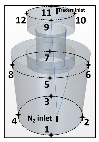
Figure 4.
Schematic diagram of location of 12 monitor points (marked by numbers), gas inlet and tracer inlet.
Figure 5 shows the mixing time of the monitor points at the top of the ladle in the physical modeling calculated by the 95% mixing standard. The dosage of saturated KCl solution tracer is 40 mL, 60 mL, 80 mL, 100 mL and 150 mL. At monitor point 5, the mixing time gradually decreases with the increase in tracer dosage. At monitor point 6 and point 8, the mixing time first decreases and gradually increases with the increase in tracer dosage. The switch points of tracer dosage are 100 mL and 80 mL for two monitor points, respectively. In addition, at monitor points 5, 6 and 8, the mixing time of 150 mL KCl tracer case is significantly shorter than that of the 40 mL KCl tracer case, with the error ranges of 61.2%, 21% and 22%, respectively.
Figure 5.
Comparison of the mixing time of different dosages of KCl solution in the water model.
3.2. Numerical Simulation Validation
Figure 6 shows the comparison of the dimensionless concentration-time curves between numerical simulation and physical modeling at the top of the ladle. It can be seen that the two curves agree well at monitor points 5 and 8. At monitor point 6, the curves deviate somehow, and this result was also reported in a recent work [52]. In all, the present model can be reasonably used to predict the mixing phenomena and fluid flow in the water model of the SSRF degasser.
Figure 6.
Comparison of dimensionless concentration-time curves between numerical simulation and physical modeling. (a1) 40 mL point 5, (b1) 40 mL point 6, (c1) 40 mL point 8, (a2) 60 mL point 5, (b2) 60 mL point 6, (c2) 60 mL point 8, (a3) 80 mL point 5, (b3) 80 mL point 6, (c3) 80 mL point 8, (a4) 100 mL point 5, (b4) 100 mL point 6, (c4) 100 mL point 8, (a5) 150 mL point 5, (b5) 150 mL point 6, and (c5) 150 mL point 8.
3.3. Transport Process of Tracer in Water Model
In the following part, the transport process of the passive scalar tracer in the water model of SSRF will be discussed. The evolution of the streamline of passive scalar in the water model at different time steps is shown in Figure 7. Accordingly, a schematic diagram of the transport process of the tracer in the water model of SSRF is shown in Figure 8.
Figure 7.
Evolution of streamlines of the passive scalar tracer in the water model of SSRF. (a) 3 s, (b) 8 s, (c) 14 s, (d) 17 s, (e) 29 s, (f) 41 s, (g) 65 s, and (h) 77.06 s.
Figure 8.
Schematic diagram of transport process of tracers in the water model of SSRF (Three paths are denoted A, B and C).
The specific transport process is described as follows. First, the injected tracer diffuses to the left side along the top surface of the vacuum chamber. Then, the tracer that is located at the left side of the upper parts of the vacuum chamber flows downward along the left side of the snorkel and finally disperses to the bottom of the ladle. Furthermore, a large portion of the tracer at the bottom of the ladle flows upward to the snorkel and the top surface of the vacuum chamber. The aforementioned downward-flow and up-flow form a main circulation stream (Path A) in the SSRF. After circulated to the top surface, the tracer continues to perform the next circulation. In addition, in both Path B and Path C, after the first main circulation (about 10 s), a small portion of tracer at the bottom of the ladle flows upward to the gap between the snorkel and the ladle at the right side. The tracers have reached the monitor point 6, as shown in Figure 4. Thereafter, the tracers start to flow to the gap between the snorkel and the ladle at the left side, for example, monitor point 8. Specifically, the tracer flows either clockwise or anti-clockwise near the top surface of the ladle, as shown in Path B and Path C, respectively. After being transported to monitor 8, the tracers diffuse to the bottom of the ladle again. Then, the tracers flow upward to start the next circulation. Finally, the homogenization of the tracer in the water model of SSRF is achieved at about 77.06 s, as shown in Figure 7h.
The specific transport process of KCl tracer (tracer disperses from the top of the vacuum chamber to the snorkel, and then disperses at the bottom of the ladle, and finally diffuses to the top of the ladle) will be discussed in Section 3.4.2.
3.4. Comparison of Fluid Flow and Transport Process of Tracers in the Case of 20 mL KCl Tracer and the Case of 150 mL KCl Tracer
In the following part, taking the case of 20 mL and 150 mL saturated KCl solution tracer as examples, the difference in their tracer dosage is 7.5 times. These are two extreme cases. The flow field, tracer transport process and mixing time under the two cases are compared.
3.4.1. Comparison of Flow Field in Water Model after Adding 20 mL and 150 mL KCl Tracer
Figure 9 shows the comparison of the flow field between the two cases at the central longitudinal section of SSRF at different time steps. It can be seen from Figure 9(a1–a3,b1–b3) that the downward stream deviated to the axial center of the ladle. The velocity of downward flow in the flow field of both cases is gradually increasing, and the velocity of downward flow of 20 mL and 150 mL KCl tracer cases reaches the maximum at 12.62 s and 10.01 s, respectively. However, comparing Figure 9(a3,b3), it is found that the high velocity area of downward flow of the 150 mL KCl case is closer to the bottom of the ladle. At 29 s, it is similar for the flow field between the two cases.
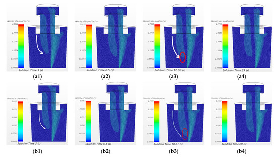
Figure 9.
Comparison of flow field between the case of 20 mL KCl tracer and the case of 150 mL KCl tracer in the water model at the central longitudinal section of SSRF at different time steps. (a1) 20 mL 3 s, (a2) 20 mL 6.5 s, (a3) 20 mL 12.62 s, (a4) 20 mL 29 s, (b1) 150 mL 3 s, (b2) 150 mL 6.5 s, (b3) 150 mL 10.01 s, and (b4) 150 mL 29 s.
3.4.2. Comparison of Transport Processes of Tracers of the Case of 20 mL KCl Tracer and the Case of 150 mL KCl Tracer in Water Model
As shown in Figure 10, the three cross sections are located at 0.01 m, 0.45 m and 0.88 m above the bottom of the ladle and named as A1–A1, A2–A2 and A3–A3, respectively. Specifically, the A1–A1 cross section is located at 0.01 m above the monitor points 1 to 4. The A2–A2 cross section is located at the same level of monitor points 5 to 8 in the ladle. The A3–A3 cross section is located at 0.02 m below the monitor points 9 to 12 in the vacuum chamber.
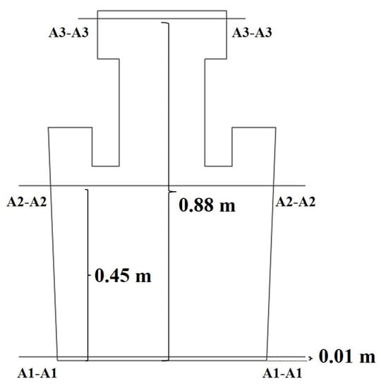
Figure 10.
Schematic diagram of the monitoring cross section.
The comparison of the dimensionless concentration-time curves between the two cases at monitor points 9 to 12 (top surface of the vacuum chamber) is shown in Figure 11. It is obvious that the peak value (or first peak value if it has two) of the curve of the 20 mL KCl tracer case at monitor points 9 to 12 is higher than that of the 150 mL KCl tracer case. However, the start-mixing time is almost the same for the two cases. The time for the peak of the curve of 20 mL KCl tracer case at monitor points 9 to 12 is earlier than that of the 150 mL KCl tracer case. The reason for the difference in time between the peak values of dimensionless concentration-time curve of two cases is that the injection interval of 20 mL KCl case is 0.4 s, and the interval of 150 mL KCl case is 3 s.
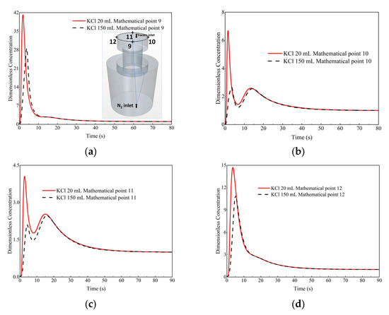
Figure 11.
Comparison of the dimensionless concentration-time curves between the case of the 20 mL KCl tracer and the case of 150 mL KCl tracer at different monitor locations. (a) Monitor point 9, (b) Monitor point 10, (c) Monitor point 11, and (d) Monitor point 12.
The variation in mass fraction of the KCl tracer of the two cases at the A3–A3 cross section (close to the top of the vacuum chamber) at different time steps is shown in Figure 12. The area of the highest mass fraction of tracer of 20 mL KCl case moves directly to monitor point 9 (lower side of A3–A3 cross section). However, the area of the highest mass fraction of tracer of 150 mL KCl case moves directly to the left side and the lower side of the A3–A3 cross section.
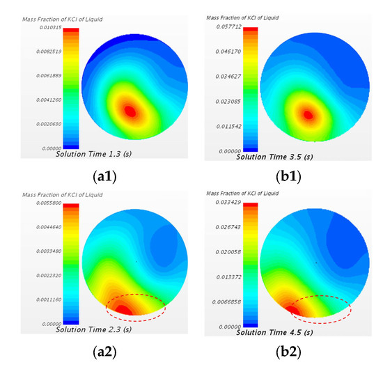
Figure 12.
Comparison of mass fraction of the KCl tracer of the case of the 20 mL KCl tracer and the case of the 150 mL KCl tracer at the A3–A3 cross section at different states. (a1) 20 mL 1.3 s, (b1) 150 mL 3.5 s, (a2) 20 mL 2.3 s, and (b2) 150 mL 4.5 s.
The variation in the mass fraction of the KCl tracer of the two cases at the central longitudinal section of SSRF at different time steps are shown in Figure 13. It can be seen from Figure 13(a2,b2) that for 20 mL KCl tracer case, most of the tracer disperses to the left side wall (near the monitor point 12) of the vacuum chamber. The injection intervals of the cases of 20 mL and 150 mL KCl tracer are 0.4 s and 3 s, respectively. Before 0.5 s and 3 s, the area of the highest mass fraction of tracer of 20 mL and 150 mL KCl cases is near the tracer inlet. The dispersion of tracer is delayed for a large dosage of tracer case. Then, the tracers flow downward to the snorkel and the ladle, and the diffusion front of the two cases reaches the ladle bottom at 8.45 s and 8.63 s, respectively. In both cases, the tracer almost simultaneously disperses to the bottom of the ladle regardless the initial injection time interval differences. The delayed injection time is shortened after the tracer flow downward to the bottom of ladle. It also indicates that the transport process of the 150 mL KCl tracer case is faster than that of the 20 mL KCl tracer case.
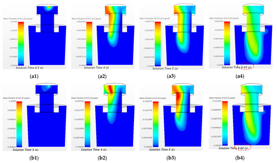
Figure 13.
Comparison of mass fraction of KCl tracer of the case of 20 mL KCl tracer and the case of 150 mL KCl tracer at the central longitudinal section of SSRF at different time steps. (a1) 20 mL 0.5 s, (a2) 20 mL 4 s, (a3) 20 mL 5 s, (a4) 20 mL 8.45 s, (b1) 150 mL 3 s, (b2) 150 mL 4 s, (b3) 150 mL 5 s, and (b4) 150 mL 8.63 s.
The comparison of the dimensionless concentration-time curves between the two cases at monitor points 1 to 4 (bottom of the ladle) is shown in Figure 14. During 15 s to 30 s, the dimensionless concentration-time curve of 150 mL KCl tracer case at monitor points 1 to 3 rises rapidly than that of 20 mL KCl tracer case. At monitor points 1, 3 and 4, the difference of dimensionless concentration curves between 20 mL and 150 mL KCl tracer cases is not obvious. Surprisingly, at monitor point 2, the curve of 150 mL KCl tracer case shifts to the left and upper side of that of 20 mL KCl tracer case, i.e., the peak value is higher and the peak time is earlier than that of 20 mL KCl tracer case. It can be explained that in the 150 mL KCl tracer case, the tracer flow downwards from vacuum chamber to the bottom of the ladle at a higher pace than that of 20 mL KCl tracer case.
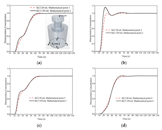
Figure 14.
Comparison of the dimensionless concentration-time curves between the case of 20 mL KCl tracer and the case of 150 mL KCl tracer at different monitor locations. (a) Monitor point 1, (b) Monitor point 2, (c) Monitor point 3, and (d) Monitor point 4.
Figure 15 shows that the variation of mass fraction of KCl tracer of the two cases at A1–A1 cross section (close to the bottom of the ladle) at different time. It can be seen from Figure 15(a1–a3,b1–b3) that, during 11 s to 23 s, the area of the highest mass fraction of tracer is moving from the central part to the right part of A1–A1 cross section (monitor point 2). It indicates that the tracer first disperses to the right side of the bottom of the ladle. It can be seen from Figure 15(a4,b4) that at 29.6 s, the tracer will gradually fill the bottom of the ladle. The difference of distribution of mass fraction of tracer between two cases is significant. During 11 s to 29.6 s, the mass fraction of tracer of 20 mL KCl case is uniform at the bottom of the ladle, while the area of the highest mass fraction of tracer of 150 mL KCl case is located on the right side of the bottom of the ladle (monitor point 2). There may exist a “dead zone”.
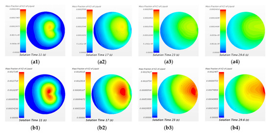
Figure 15.
Comparison of mass fraction of KCl tracer of the case of 20 mL KCl tracer and the case of 150 mL KCl tracer at A1-A1 cross section at different time steps. (a1) 20 mL 11 s, (a2) 20 mL 17 s, (a3) 20 mL 23 s, (a4) 20 mL 29.6 s, (b1) 150 mL 11 s, (b2) 150 mL 17 s, (b3) 150 mL 23 s, and (b4) 150 mL 29.6 s.
The comparison of the dimensionless concentration-time curves between the two cases at monitor points 5 to 8 (top of the ladle) is shown in Figure 16. The start-mixing time of 20 mL and 150 mL KCl tracer cases is basically the same. At monitor points 5 to 8, the peak time of dimensionless concentration-time curve of 150 mL KCl case is earlier and the peak value is higher than that of 20 mL KCl tracer case. Overall, the difference between two cases is not obvious.
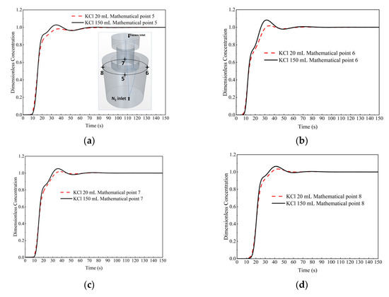
Figure 16.
Comparison of the dimensionless concentration-time curves between the case of 20 mL KCl tracer and the case of 150 mL KCl tracer at different monitor locations. (a) Monitor point 5, (b) Monitor point 6, (c) Monitor point 7, and (d) Monitor point 8.
The variation of mass fraction of KCl tracer of two cases at A2–A2 cross section (close to the top surface of the ladle) at different time steps are shown in Figure 17. At 11 s, the area of the highest mass fraction of tracer is located at the center of the A2–A2 cross section (downflow stream of the snorkel). During 11 s to 41 s, the mass fraction of tracer on the right side of the section (monitor point 6) increases first, then the mass fraction of tracer on the upper and lower sides of the section (monitor points 7 and 5) increases, and finally the mass fraction of tracer on the left side of the section (monitor point 8) increases, which corresponds to two side circulation streams of the transport process, as described earlier in Figure 8. At 29 s and 41 s, the distribution of mass fraction of KCl tracer at A2–A2 cross section is similar between two cases. In other words, the dosages of tracer have a slight effect on the transport rate of tracers that transport from the bottom to the top of the ladle.
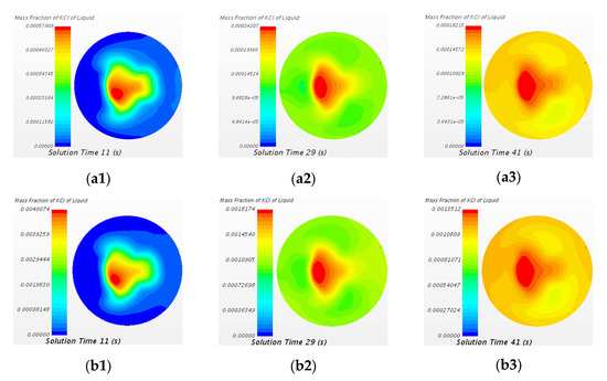
Figure 17.
Comparison of mass fraction of KCl tracer of the case of 20 mL KCl tracer and the case of 150 mL KCl tracer at A2-A2 cross section at different time steps. (a1) 20 mL 11 s, (a2) 20 mL 29 s, (a3) 20 mL 41 s, (b1) 150 mL 11 s, (b2) 150 mL 29 s, and (b3) 150 mL 41 s.
3.4.3. Comparison of the Mixing Time
The mixing time which employed 99% mixing standard at each monitor point is summarized in Table 4. When comparing the dosage of 20 mL and 150 mL KCl tracer cases, the mixing time of 150 mL KCl tracer case is slightly shorter than that of 20 mL KCl tracer case at monitor points 9 to 12, and the difference is not significant. Specifically, the error range is less than 2%. At monitor points 1 to 5, the mixing time of 150 mL KCl tracer case is obviously shorter than that of 20 mL KCl tracer case, and the error range is 28.2%, 5.5%, 6%, 11.7% and 4.7%, respectively. However, at monitor point 6 and 8, the difference of mixing time can be neglected. On the contrary, the mixing time of 150 mL KCl tracer case is significantly longer than that of 20 mL KCl tracer case at monitor point 7, the error range is 38.2%.
Table 4.
Mixing time at all monitor points (Point is abbreviated as P).
When comparing KCl and pure water cases, i.e., to evaluate the effect of tracer density, the mixing time of 150 mL KCl tracer case is slightly shorter than that of 150 mL pure water tracer case at monitor points 9 to 12, the error range is less than 4%. At monitor points 1, 3, 4, and the mixing time of 150 mL KCl tracer case is obviously shorter than that of 150 mL pure water tracer case, and the error range is 12% to 24%. However, at monitor point 2, the mixing time of 150 mL KCl tracer case is longer than that of 150 mL pure water tracer case, with an error of 34%. This may be due to the presence of a “dead zone” at the right side of the bottom of the ladle. At monitor points 5 to 8, the mixing time of 150 mL pure water tracer case is shorter than that of 150 mL KCl tracer case. The relative errors at monitor point 5, 6 and 8 are 2%, 10% and 5%, respectively. The difference is obvious at monitor point 7, and the error is 56%.
In summary, at the top of the vacuum chamber, the mixing time of 150 mL KCl tracer case is slightly shorter than that of 20 mL KCl tracer case and that of 150 mL pure water tracer case. At the bottom of the ladle, the mixing time of 150 mL KCl tracer case is significantly shorter than that of 20 mL KCl tracer case, and also significantly shorter than that of 150 mL pure water tracer case (except monitor point 2). At the top of the ladle, the mixing time of 20 mL KCl tracer case and 150 mL KCl tracer case is very close (except monitor point 7), and the mixing time of 150 mL pure water tracer case is shorter than that of 150 mL KCl tracer case (especially at monitor point 7). The mixing time of all salt tracer dosage cases will be compared later.
3.5. Comparison of Dimensionless Concentration-Time Curves of Different Dosages of KCl Solution Tracers
Figure 18 shows a comparison of the dimensionless concentration-time curves of the KCl solution cases with different dosages (20 mL, 40 mL, 60 mL, 80 mL, 100 mL, 150 mL, and 250 mL) at different monitor locations (monitor points 9–12). At the top of the vacuum chamber (monitor points 9 to 12), with the increase in tracer dosage, the curve shifts to the right side, i.e., the peak value of the dimensionless concentration-time curve of the corresponding tracer case is decreasing, and the time required to reach the peak is delayed. In Figure 18b,c, at monitoring points 10 and 11, when the tracer dosage increases from 150 mL to 250 mL, the difference in the first peak of the dimensionless concentration-time curve is small, but the second peak of the dimensionless concentration-time curve of 250 mL KCl case is lower than that of 150 mL KCl case. The second peak time of the dimensionless concentration-time curve of 250 mL KCl case is also longer than that of 150 mL KCl case. When the tracer dosage is increased from 150 mL to 250 mL, the circulation is delayed.
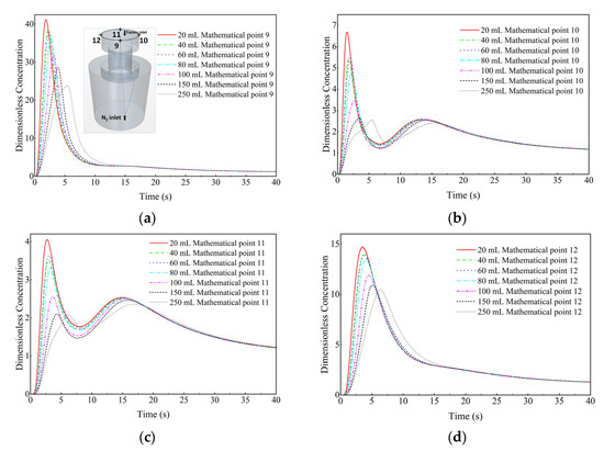
Figure 18.
Comparison of the dimensionless concentration-time curves of the KCl solution cases with different dosages at different monitor locations. (a) Monitor point 9, (b) Monitor point 10, (c) Monitor point 11, and (d) Monitor point 12.
Figure 19 is the comparison of the dimensionless concentration-time curves of the KCl solution cases with different dosages at monitor points 1 to 4. It can be seen that, at monitor point 2 (right side at the bottom of the ladle), with the increase in tracer dosage, the peak value of the dimensionless concentration-time curve of the corresponding tracer case is increased. At monitor points 1 and 3, when the tracer dosage increases from 150 mL to 250 mL, an obvious peak appears in the dimensionless concentration-time curve at about 25 s. However, at monitor point 4, the concentration-time curves are basically not affected by the different tracer dosages.
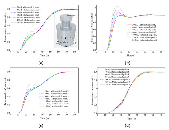
Figure 19.
Comparison of the dimensionless concentration-time curves of the KCl solution cases with different dosages at different monitor locations. (a) Monitor point 1, (b) Monitor point 2, (c) Monitor point 3, and (d) Monitor point 4.
Figure 20 shows a comparison of the dimensionless concentration-time curves of the KCl solution cases with different dosages at monitor points 5 to 8. It can be seen that, at the top of the ladle, with the increase in tracer dosage, the peak of dimensionless concentration-time curve will gradually increase. However, the difference is not obvious, and the tracer dosages has a small effect on the dimensionless concentration-time curve.
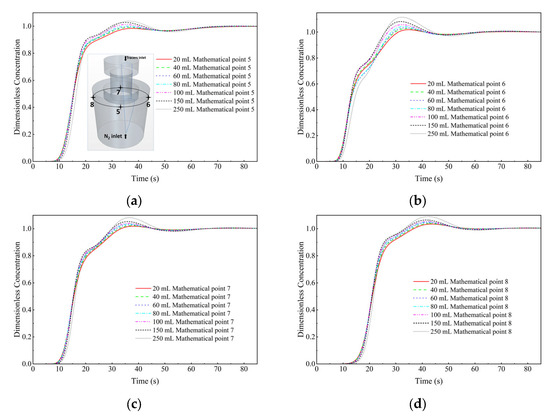
Figure 20.
Comparison of the dimensionless concentration-time curves of the KCl solution cases with different dosages at different monitor locations. (a) Monitor point 5, (b) Monitor point 6, (c) Monitor point 7, and (d) Monitor point 8.
3.6. Comparison of Mixing Time of Different Dosages of KCl Solution Tracers
Figure 21 shows the comparison of the mixing time of KCl solution at different monitor positions and different tracer dosages in the numerical simulation calculated with the 99% mixing standard. It can be seen from the figure that the mixing time at the top of the vacuum chamber (monitor points 9, 10 and 12) is the highest, the mixing time at the top of the ladle (monitor points 5, 6 and 8) is the lowest, and the mixing time at the bottom of the ladle (monitor points 1, 2 and 4) is between the above-mentioned two positions. The top area of the ladle usually corresponds to the sampling position in industrial production. The mixing time at the top of the ladle is shorter than that at the other locations of the ladle. This means that the top of ladle cannot represent the mixing state in the ladle, and sampling in this area may not be representative.
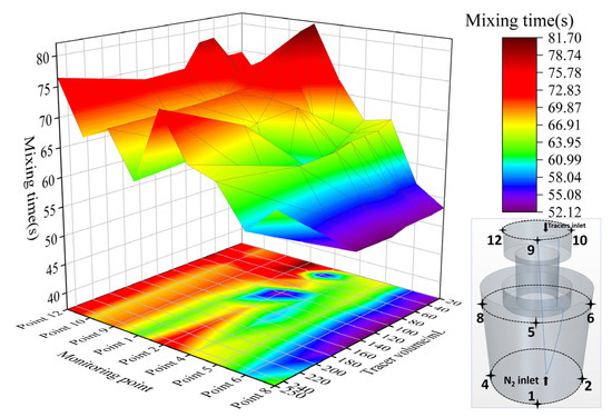
Figure 21.
Comparison of the mixing time of different dosages of the KCl solution at different monitor locations.
At the top of the vacuum chamber, the mixing time decreases slightly with the increase in tracer dosage at monitor points 9 and 10. Taking the monitor point 9 as an example, i.e., in front of the top of the vacuum chamber, the mixing time of 250 mL KCl tracer case is slightly shorter than that of 20 mL KCl tracer case, and the error range is 2.5%. At monitor point 12 on the left, the mixing time is almost constant with the increase in tracer dosage.
At the bottom of the ladle, at monitor point 1 in the front side, the mixing time decreases with the increase in tracer dosage. The mixing time of 250 mL KCl tracer case is significantly shorter than that of 20 mL KCl tracer case, and the error range is 30.7%. At monitor point 4, the mixing time also gradually decreases with the increase in tracer dosage, the mixing time of 150 mL KCl tracer case is shorter than that of 20 mL KCl tracer case, and the error range is 11.7%. However, when the tracer dosage increases from 150 mL to 250 mL, the mixing time begins to increase, with the error range of 13.%. At monitor point 2, the dosage of tracer has small effect on the mixing time. However, when the tracer dosage increases from 150 mL to 250 mL, the mixing time will also increase by 8.8%.
At the top of the ladle, at monitor point 5 in the front side, when the dosage of KCl tracer increases from 20 mL to 150 mL, the mixing time gradually decreases, but when it increases from 150 mL to 250 mL, the mixing time increases slightly, with the error range of 2.8%. At monitor points 6 and 8, the mixing time is almost constant with the increase in tracer dosage. However, when the dosage of KCl tracer increases from 150 mL to 250 mL, the mixing time increases, with the error range of 4.7% and 21.7%, respectively. This indicates that the mixing time increases when the tracer dosage is large. This tendency is similar to the water model experimental results, as described in Section 3.1.
In short, with the increase in tracer dosage, the mixing time of the top of the vacuum chamber decreases gradually, but the percentage is small. The mixing time of the bottom of the ladle decreases significantly with the increase in tracer dosage. However, in part of this area (dead zone), the mixing time will increase when the tracer dosage is large. The mixing time of the top of the ladle decreases first and then increases when increasing the tracer dosage, which is similar to the water model experimental results.
4. Conclusions
- The water model experimental results show that in some areas at the top of the ladle, the mixing time decreases first and then increases when increasing the tracer dosage. In addition, the mixing time of the top area of the ladle with large tracer dosage is shorter than that with small tracer dosage. Taking the area on the front side of the top of the ladle as an example, the mixing time of 150 mL KCl tracer case is significantly shorter than that of 40 mL KCl tracer case, and the error range is 61.2%.
- For the transport process of two different dosage of KCl tracer cases, compared with 20 mL KCl tracer case, in the 150 mL KCl tracer case, the tracer flow downwards at a higher pace from the vacuum chamber to the bottom of the ladle. This may compensate the injection time interval of large dosage cases. Additionally, the mass fraction of KCl tracer of 150 mL KCl tracer case is the highest at the right side of the bottom of the ladle which might be a “dead zone”.
- At the top of the vacuum chamber, with the increase in tracer dosage, the dimensionless concentration-time curve shifts to the right side, i.e., the peak value is decreasing, and the time required to reach the peak is delayed. At the bottom of the ladle, with the increase in tracer dosage, the peak value of the dimensionless concentration-time curve is increased. At the top of the ladle, with the increase in the dosage of tracer, the peak value of the dimensionless concentration-time curve will also gradually increase, but the difference is not obvious.
- With the increase in tracer dosage, the mixing time of the top of the vacuum chamber decreases gradually, but the change is not obvious. The mixing time of the bottom of the ladle decreases significantly with the increase in tracer dosage. However, in the dead zone, the mixing time will increase when the tracer dosage is large. The mixing time of the top of the ladle decreases first and then increases when increasing the tracer dosage.
- In addition, the mixing time of the top of the ladle is the shortest, which means that sampling at the top of the ladle in industrial production cannot represent the entire mixing state in the ladle.
Author Contributions
Conceptualization, C.C. and G.C.; methodology, W.L., Y.L., Y.Z. and C.C.; software, Y.Z. and X.O.; investigation Y.L., Y.Z. and C.C.; resources, W.L., C.C. and G.C.; data curation, X.O. and Y.Z.; writing—original draft preparation, X.O. and Y.Z.; writing—review and editing, W.L., Y.L., J.F., C.C. and G.C.; supervision, W.L., C.C. and G.C.; funding acquisition, C.C. All authors have read and agreed to the published version of the manuscript.
Funding
This research was funded by National Natural Science Foundation of China, grant number 51904204, and Research Project Supported by Shanxi Scholarship Council of China, grant number 2022-040.
Data Availability Statement
Not applicable.
Acknowledgments
The anonymous reviewers are acknowledged for their valuable comments.
Conflicts of Interest
The authors declare no conflict of interest.
References
- Cheng, G.G.; Rui, Q.X.; Qin, Z.; Zhang, J. Development and Application of Single Snorkel Refining Furnace. China Metall. 2013, 23, 1–10. [Google Scholar] [CrossRef]
- Kitamura, S.; Aoki, H.; Miyamoto, K.; Furuta, H.; Yamashita, K.; Yonezawa, K. Development of a Novel Degassing Process Consisting with Single Large Immersion Snorkel and a Bottom bubbling ladle. ISIJ Int. 2000, 40, 455–459. [Google Scholar] [CrossRef]
- Jönsson, P.G.; Jonsson, L.T.I. The Use of Fundamental Process Models in Studying Ladle Refining Operations. ISIJ Int. 2001, 41, 1289–1302. [Google Scholar] [CrossRef]
- Cao, J.Q.; Chen, C.; Xue, L.Q.; Li, Z.; Zhao, J.; Lin, W.M. Analysis of the inclusions in the whole smelting process of non-oriented silicon steel DG47A. Iron Steel 2022. accepted. [Google Scholar]
- Meng, Y.Q.; Li, J.L.; Zhu, H.Y.; Wang, K.P. Effect of LF soft bubbling time on oxide inclusions in Si-killed spring steel. Iron Steel 2022, 57, 48–54. [Google Scholar] [CrossRef]
- Jiang, X.F.; Peng, F.; Zhang, Y.L.; Xue, W.H. Application of carbon deoxidation in ladle top slag modification. Iron Steel 2020, 55, 43–48. [Google Scholar] [CrossRef]
- Chattopadhyay, K.; Morales-Davila, R.; Nájera-Bastida, A.; Rodríguez-Ávila, J.; Muñiz-Valdés, C.R. Numerical Simulation of Melting Kinetics of Metal Particles during Tapping with Argon-Bottom Stirring. Crystals 2020, 10, 901. [Google Scholar] [CrossRef]
- Li, Y.H.; He, Y.B.; Ren, Z.F.; Bao, Y.P.; Wang, R. Comparative Study of the Cleanliness of Interstitial-Free Steel with Low and High Phosphorus Contents. Steel Res. Int. 2021, 92, 2000581. [Google Scholar] [CrossRef]
- Ma, G.J.; Liu, M.K.; Zhang, X.; Zheng, D.L.; Yao, W.L. Research Progress on Melting Behavior of Steel Scrap in Iron-Carbon Bath. Iron Steel 2022, 57, 1–11. Available online: https://kns.cnki.net/kcms/detail/11.2118.TF.20220127.0956.001.html (accessed on 30 October 2022).
- Conejo, A.N. Physical and Mathematical Modelling of Mass Transfer in Ladles due to Bottom Gas Stirring: A Review. Processes 2020, 8, 750. [Google Scholar] [CrossRef]
- Jardón-Pérez, L.E.; González-Rivera, C.; Ramirez-Argaez, M.A.; Dutta, A. Numerical Modeling of Equal and Differentiated Gas Injection in Ladles: Effffect on Mixing Time and Slag Eye. Processes 2020, 8, 917. [Google Scholar] [CrossRef]
- Riabov, D.; Gain, M.M.; Kargul, T.; Volkova, O. Influence of Gas Density and Plug Diameter on Plume Characteristics by Ladle Stirring. Crystals 2021, 11, 475. [Google Scholar] [CrossRef]
- Haas, T.; Schubert, C.; Eickhoff, M.; Pfeifer, H. A Review of Bubble Dynamics in Liquid Metals. Metals 2021, 11, 664. [Google Scholar] [CrossRef]
- Hu, Q.; Li, X.S.; Zhang, J.Q.; Lian, Y.X.; Tang, H.Y. Effect of differential flowrate argon blowing mode on mixing and top slag behavior for a 150 t ladle. Iron Steel 2020, 55, 31–38. [Google Scholar] [CrossRef]
- Tang, W.D.; Tang, H.Y. Mathematical Simulation of Effect of Nozzle Eccentricity on Ladle Teeming Process. Iron Steel 2021, 56, 75–85. [Google Scholar] [CrossRef]
- Zhang, D.; Chen, C.; Zhang, Y.X.; Wang, S.B. Numerical simulation of tracer transport process in water model of gas-stirred ladle. J. Taiyuan Univ. Technol. 2020, 51, 50–58. [Google Scholar] [CrossRef]
- Qi, H.Y.; Chen, C.; Xue, L.Q.; Yang, R.W.; Ni, P.Y.; Yin, L.F.; Xin, Y.J. Numerical Simulation of Tracer Transport Process in Alternate Stirring Ladle. J. Taiyuan Univ. Technol. 2022, 1–11. Available online: https://kns.cnki.net/kcms/detail/14.1220.N.20220314.1038.006.html (accessed on 30 October 2022).
- Yang, R.W.; Chen, C.; Lin, Y.C.; Zhao, Y.; Zhao, J.; Zhu, J.J.; Yang, S.S. Water model experiment on motion and melting of scarp in gas stirred reactors. Chin. J. Process Eng. 2022, 22, 954–962. [Google Scholar] [CrossRef]
- Zhu, J.J.; Chen, C.; Fan, J.P.; Li, L.B.; Chen, M.; Yang, H.B.; Lin, W.M. Study on motion melting and mixing of ice samples in a water model of ladle. J. Taiyuan Univ. Technol. 2022, 1–10. Available online: https://kns.cnki.net/kcms/detail/14.1220.N.20221027.1430.002.html (accessed on 30 October 2022).
- Seshadri, V.; Costa, S.L.D.S. Cold Model Studies of R. H. Degassing Process. Trans. ISIJ 1986, 26, 133–138. [Google Scholar] [CrossRef]
- Li, B.K.; Tsukihashi, F. Modeling of Circulating Flow in RH Degassing Vessel Water Model Designed for Two- and Multi-Legs Operations. ISIJ Int. 2000, 40, 1203–1209. [Google Scholar] [CrossRef]
- Luo, Y.; Liu, C.; Ren, Y.; Zhang, L.F. Modeling on the Fluid Flow and Mixing Phenomena in a RH Steel Degasser with Oval Down-Leg Snorkel. Steel Res. Int. 2018, 89, 1800048. [Google Scholar] [CrossRef]
- Li, Y.H.; Zhu, H.W.; Wang, R.; Ren, Z.F.; Lin, L. Prediction of two phase flow behavior and mixing degree of liquid steel under reduced pressure. Vacuum 2021, 192, 110480. [Google Scholar] [CrossRef]
- Ling, H.T.; Li, F.; Zhang, L.F.; Conejo, A.N. Investigation on the Effect of Nozzle Number on the Recirculation Rate and Mixing Time in the RH Process Using VOF+DPM Model. Metall. Mater. Trans. B 2016, 47, 1950–1961. [Google Scholar] [CrossRef]
- Li, Y.H.; Zhu, H.W.; Wang, R.; Ren, Z.F.; He, Y.B. Bubble behavior and evolution characteristics in the RH riser tube-vacuum chamber. Int. J. Chem. React. Eng. 2022, 20, 1053–1064. [Google Scholar] [CrossRef]
- Zhao, Z.J.; Wang, M.; Song, L.; Bao, Y.P. Splashing Simulation of Liquid Steel Drops during the Ruhrstahl Heraeus Vacuum Process. Metals 2020, 10, 1070. [Google Scholar] [CrossRef]
- Wei, G.S.; Dong, J.F.; Zhu, R.; Han, B.C. Effect of ladle bottom blowing on RH dehydrogenation and inclusions. Iron Steel 2021, 56, 63–68. [Google Scholar] [CrossRef]
- Chen, G.J.; Yang, J.; Li, L.; Zhang, M.; He, S.P. Metallurgical reaction behavior of Ar-CO2 mixed injection during RH refining process. Iron Steel 2022, 57, 55–60. [Google Scholar] [CrossRef]
- Zhu, G.S.; Deng, X.X.; Ji, C.X. Effect of vacuum degree on inclusion removal in ultra low carbon steel during RH refining process. Iron Steel 2022, 1–8. [Google Scholar] [CrossRef]
- Liu, C.; Zhang, L.F.; Li, F.; Peng, K.Y.; Liu, F.G.; Liu, Z.T.; Zhao, Y.Y.; Yang, W.; Zhang, J. Water Modeling on Circulating Flow and Mixing Time in a Ruhrstahl–Heraeus Vacuum Degasser. Steel Res. Int. 2021, 92, 2000608. [Google Scholar] [CrossRef]
- Liu, C.; Zhang, L.F.; Sun, Y.; Yang, W. Large Eddy Simulation on the Transient Decarburization of the Molten Steel During RH Refining Process. Metall. Mater. Trans. B 2022, 53, 670–681. [Google Scholar] [CrossRef]
- Chen, G.J.; He, S.P. Hydrodynamic Modeling of Two-Phase Flow in the Industrial Ruhrstahl–Heraeus Degasser: Effect of Bubble Expansion Models. Metall. Mater. Trans. B 2022, 53, 208–219. [Google Scholar] [CrossRef]
- Wang, R.D.; Jin, Y.; Cui, H. The Flow Behavior of Molten Steel in an RH Degasser Under Different Ladle Bottom Stirring Processes. Metall. Mater. Trans. B 2022, 53, 342–351. [Google Scholar] [CrossRef]
- Dai, W.X.; Cheng, G.G.; Li, S.J.; Huang, Y.; Zhang, G.L.; Qiu, Y.L.; Zhu, W.F. Numerical Simulation of Multiphase Flow and Mixing Behavior in an Industrial Single Snorkel Refining Furnace (SSRF): The Effect of Gas Injection Position and Snorkel Diameter. ISIJ Int. 2019, 59, 1214–1223. [Google Scholar] [CrossRef]
- Rui, Q.X.; Jiang, F.; Ma, Z.; You, Z.M.; Cheng, G.G.; Zhang, J. Effect of Elliptical Snorkel on the Decarburization Rate in Single Snorkel Refining Furnace. Steel Res. Int. 2013, 84, 192–197. [Google Scholar] [CrossRef]
- Dai, W.X.; Cheng, G.G.; Li, S.J.; Huang, Y.; Zhang, G.L. Numerical Simulation of Multiphase Flow and Mixing Behavior in an Industrial Single Snorkel Refining Furnace (SSRF): Effect of Bubble Expansion and Snorkel Immersion Depth. ISIJ Int. 2019, 59, 2228–2238. [Google Scholar] [CrossRef]
- Zhang, Y.X.; Chen, C.; Lin, W.M.; Yu, Y.C.; E, D.Y.; Wang, S.B. Numerical Simulation of Tracers Transport Process in Water Model of a Vacuum Refining Unit: Single Snorkel Refining Furnace. Steel Res. Int. 2020, 91, 2000022. [Google Scholar] [CrossRef]
- Levenspiel, O. Tracer Technology; Springer: New York, NY, USA, 2012. [Google Scholar]
- Haynes, W.M. (Ed.) Concentrative Properties of Aqueous Solutions: Density, Refractive Index, Freezing Point Depression, and Viscosity. In CRC Handbook of Chemistry and Physics, 93rd ed.; CRC Press: Boca Raton, FL, USA, 2012; Volume 5, p. 137. [Google Scholar]
- Geng, D.Q.; Zhang, X.; Liu, X.A.; Wang, P.; Liu, H.T.; Chen, H.M.; Dai, C.M.; Lei, H.; He, J.C. Simulation on Flow Field and Mixing Phenomenon in Single Snorkel Vacuum Degasser. Steel Res. Int. 2015, 86, 724–731. [Google Scholar] [CrossRef]
- Chen, H.M. Mathematical and Physical Simulation for Single Snorkel RH Vacuum Refining Process. Master’s Thesis, Northeastern University, Shenyang, China, 2014. [Google Scholar]
- Wei, J.H.; Jiang, X.Y.; Wen, L.J.; Li, B. Mass Transfer Characteristics between Molten Steel and Particles under Conditions of RH-PB(IJ) Refining Process. ISIJ Int. 2007, 47, 408–417. [Google Scholar] [CrossRef][Green Version]
- Mukherjee, D.; Shukla, A.K.; Senk, D.G. Cold Model-Based Investigations to Study the Effects of Operational and Nonoperational Parameters on the Ruhrstahl–Heraeus Degassing Process. Metall. Mater. Trans. B 2017, 48, 763–771. [Google Scholar] [CrossRef]
- Chen, C.; Cheng, G.G.; Sun, H.B.; Hou, Z.B.; Wang, X.C.; Zhang, J.Q. Effects of salt tracer amount, concentration and kind on the fluid flow behavior in a hydrodynamic model of continuous casting tundish. Steel Res. Int. 2012, 83, 1141–1151. [Google Scholar] [CrossRef]
- Chen, C.; Jonsson, L.T.I.; Tilliander, A.; Cheng, G.G.; Jönsson, P.G. A mathematical modeling study of tracer mixing in a continuous casting tundish. Metall. Mater. Trans. B 2015, 46, 169–190. [Google Scholar] [CrossRef]
- Chen, C.; Jonsson, L.T.I.; Tilliander, A.; Cheng, G.G.; Jönsson, P.G. A mathematical modeling study of the influence of small amounts of KCl solution tracers on mixing in water and residence time distribution of tracers in a continuous flow reactor-metallurgical tundish. Chem. Eng. Sci. 2015, 137, 914–937. [Google Scholar] [CrossRef]
- Ding, C.Y.; Lei, H.; Niu, H.; Zhang, H.; Yang, B.; Zhao, Y. Effects of Salt Tracer Volume and Concentration on Residence Time Distribution Curves for Characterization of Liquid Steel Behavior in Metallurgical Tundish. Metals 2021, 11, 430. [Google Scholar] [CrossRef]
- Ding, C.Y.; Lei, H.; Niu, H.; Zhang, H.; Yang, B.; Li, Q. Effects of Tracer Solute Buoyancy on Flow Behavior in a Single-Strand Tundish. Metall. Mater. Trans. B 2021, 52, 3788–3804. [Google Scholar] [CrossRef]
- Chen, C.; Rui, Q.X.; Cheng, G.G. Effect of salt tracer amount on the mixing time measurement in a hydrodynamic model of gas-stirred ladle system. Steel Res. Int. 2013, 84, 900–907. [Google Scholar] [CrossRef]
- Gómez, A.S.; Conejo, A.N.; Zenit, R. Effect of Separation Angle and Nozzle Radial Position on Mixing Time in Ladles with Two Nozzles. J. Appl. Fluid Mech. 2018, 11, 11–20. [Google Scholar] [CrossRef]
- Qi, F.S.; Liu, J.X.; Liu, Z.Q.; Cheung, S.C.P.; Li, B.K. Characterization of the Mixing Flow Structure of Molten Steel in a Single Snorkel Vacuum Refining Furnace. Metals 2019, 9, 400. [Google Scholar] [CrossRef]
- Dai, W.X.; Cheng, G.G.; Zhang, G.L.; Huo, Z.D.; Lv, P.X.; Qiu, Y.L. Investigation of Circulation Flow and Slag-Metal Behavior in an Industrial Single Snorkel Refining Furnace (SSRF): Application to Desulfurization. Metall. Mater. Trans. B 2020, 51, 611–627. [Google Scholar] [CrossRef]
- Mondal, M.K.; Maruoka, N.; Kitamura, S.; Gupta, G.S.; Nogami, H.; Shibata, H. Study of Fluid Flow and Mixing Behaviour of a Vacuum Degasser. Trans. Indian Inst. Metals 2012, 65, 321–331. [Google Scholar] [CrossRef]
- You, Z.M.; Cheng, G.G.; Wang, X.C.; Qin, Z.; Tian, J.; Zhang, J. Mathematical Model for Decarburization of Ultra-low Carbon Steel in Single Snorkel Refining Furnace. Metall. Mater. Trans. B 2015, 46, 459–472. [Google Scholar] [CrossRef]
- Geng, D.Q.; Lei, H.; He, J.C. Decarburization and Inclusion Removal Process in Single Snorkel Vacuum Degasser. High Temp. Mat. Process. 2017, 36, 523–530. [Google Scholar] [CrossRef]
- Chen, S.F.; Lei, H.; Wang, M.; Yang, B.; Dou, W.X.; Chang, L.S.; Zhang, H.W. Ar-CO-liquid steel flow with decarburization chemical reaction in single snorkel refining furnace. Int. J. Heat Mass Transf. 2020, 146, 118857. [Google Scholar] [CrossRef]
- Wang, C.; Zhang, J.; Yang, N.Z.; Fan, G.Q.; Wang, Z.X.; Zhu, K.X.; Kou, W.T. Investigation on Water Modelling of Flow Field and Circulation Flow Rate for Single Snorkel Refining Furnace. Spec. Steel 1998, 19, 12–15. Available online: http://en.cnki.com.cn/Article_en/CJFDTOTAL-TSGA199802002.htm (accessed on 30 October 2022).
- Qin, Z.; Pan, H.W.; Zhu, M.T.; Cheng, G.G.; Zhang, J. The Flow Behavior of Molten Steel in the Process of Vacuum Treatment with Single Snorkel Refining Furnace. J. Iron Steel Res. Int. 2010, 17, 47–52. [Google Scholar]
- Yang, X.M.; Zhang, M.; Wang, F.; Duan, J.P.; Zhang, J. Mathematical Simulation of Flow Field for Molten Steel in an 80–ton Single Snorkel Vacuum Refining Furnace. Steel Res. Int. 2012, 83, 55–82. [Google Scholar] [CrossRef]
- Chen, G.J.; He, S.P. Numerical simulation of Argon–Molten steel two-phase flow in an industrial single snorkel refining furnace with bubble expansion, coalescence, and breakup. J. Mater. Res. Technol. 2020, 9, 3318–3329. [Google Scholar] [CrossRef]
- Sano, M.; Mori, K.; Fujita, Y. Dispersion of Gas Injected into Liquid Metal. Tetsu Hagané 1979, 65, 1140–1148. Available online: https://www.jstage.jst.go.jp/article/tetsutohagane1955/65/8/65_8_1140/_pdf (accessed on 30 October 2022). [CrossRef]
- Schiller, L.; Naumann, Z. A Drag Coefficient Correlation. Z. Ver. Dtsch. Ing. 1935, 77, 318–320. [Google Scholar]
- Auton, T.R. The Lift Force on a Spherical Body in a Rotational Flow. J. Fluid Mech. 1987, 183, 199–218. [Google Scholar] [CrossRef]
- Shih, T.H.; Liou, W.W.; Shabbir, A.; Yang, Z.; Zhu, J. A new k-ϵ eddy viscosity model for high reynolds number turbulent flows. Comput. Fluids 1995, 24, 227–238. [Google Scholar] [CrossRef]
- Rodi, W. Experience with two-layer models combining the k-epsilon model with a one-equation model near the wall. In Proceedings of the 29th Aerospace Sciences Meeting, Reno, NV, USA, 1–10 January 1991; ARC: Columbus, OH, USA, 1991; p. 216. [Google Scholar] [CrossRef]
- Wolfshtein, M. The velocity and temperature distribution in one-dimensional flow with turbulence augmentation and pressure gradient. Int. J. Heat Mass Transf. 1969, 12, 301–318. [Google Scholar] [CrossRef]
- Ilegbusi, O.J.; Iguchi, M.; Nakajima, K.; Sano, M.; Sakamoto, M. Modeling Mean Flow and Turbulence Characteristics in Gas-Agitated Bath with Top Layer. Metall. Mater. Trans. B 1998, 29, 211–222. [Google Scholar] [CrossRef]
- Vanýsek, P. Ionic Conductivity and Diffusion at Infinite Dilution. In CRC Handbook of Chemistry and Physics, 93rd ed.; Haynes, W.M., Ed.; CRC Press: Boca Raton, FL, USA, 2012; Volume 5, p. 77. [Google Scholar]
- Tanaka, K. Measurements of Self-diffusion Coefficients of Water in Pure Water and in Aqueous Electrolyte Solutions. J. Chem. Soc. Faraday Trans. 1 Phys. Chem. Condens. Phases 1975, 71, 1127–1131. [Google Scholar] [CrossRef]
- Coe, J.R.; Godfrey, T.B. Viscosity of Water. J. Appl. Phys. 1944, 15, 625–626. Available online: https://ui.adsabs.harvard.edu/link_gateway/1944JAP....15..625C/doi:10.1063/1.1707481 (accessed on 30 October 2022).
- Siemens. STAR-CCM+ Version 13.04 User Guide; Siemens PLM Software: Munich, Germany, 2019. [Google Scholar]
Publisher’s Note: MDPI stays neutral with regard to jurisdictional claims in published maps and institutional affiliations. |
© 2022 by the authors. Licensee MDPI, Basel, Switzerland. This article is an open access article distributed under the terms and conditions of the Creative Commons Attribution (CC BY) license (https://creativecommons.org/licenses/by/4.0/).