Article

Application of Temperature Cycles to Austenitic Steel and Study of the Residual Stresses Distribution in HAZ

Department of Engineering Technology, Faculty of Mechanical Engineering, Technical University of Liberec, Studentská 1402/2, 46117 Liberec, Czech Republic
*
Author to whom correspondence should be addressed.
Metals 2022, 12(11), 1891; https://doi.org/10.3390/met12111891
Submission received: 30 September 2022 / Revised: 26 October 2022 / Accepted: 2 November 2022 / Published: 4 November 2022

Abstract

:
This paper presents the results of research dealing with assessing the welding effect (temperature–stress cycles) on the residual stresses in these steels. Residual stresses, remaining in the material after technological processing, pose a risk, especially at the areas of local stress peaks. During the real welding, residual stresses achieve their highest values in the heat-affected zone (HAZ), which is very narrow and therefore quite problematic to be studied in detail. Therefore, a methodology of temperature–stress physical simulations has been developed to study residual stresses in the HAZ over a 6.5 times larger section of the test sample. Thus, temperature cycles corresponding to the real welding were applied to the samples in the thermo-mechanical simulator, Gleeble 3500. Subsequently, the residual stresses were determined by the X-ray diffraction method. At the same time, the influence of annealing temperature on the residual stress reduction and redistribution was also investigated. Obtained results were compared and discussed with the similar studies about HSLA and duplex steels.

1. Introduction

Austenitic steels belong to the most commonly used steels, belonging to the group of corrosion-resistant materials [1], which have already found their place in a wide range of industrial applications. They are very often used in the energy industry, e.g., in the nuclear power plants [2], but also in the aircraft industry [3], chemical and petrochemical industry [4], or in the pharmaceutical and food industry [5,6]. Fully austenitic steels have higher values of the linear thermal expansion coefficient and lower values of the thermal conductivity compared to the common structural steels, and that is why they reveal higher deformation during welding. Thanks to their high toughness, deformation arising during welding can be eliminated either by rigid clamping of given parts or by the stiffness of structure. However, this procedure also generates, in the weld and in its vicinity, the residual stresses with significant stress peaks, which have a negative effect on the fatigue life of parts [7].
During welding of all structural types of steels, but also during their static and dynamic loading, there are residual stresses generated, which are either macroscopic or microscopic [8,9]. Macroscopic stresses are mostly generated in areas larger than 1 mm and are usually caused by the technological processing or mechanical loading [10]. During the residual stresses’ analysis, the different types of stresses can be distinguished and measured individually, thus obtaining results of macroscopic and microscopic stresses [11]. Determination of the residual stresses can be performed by destructive and non-destructive methods (NDT), whereby residual stresses are measured at the sample surface or a stress gradient in the thickness direction of material is determined. In principle, the residual stresses are then determined in the longitudinal and transverse directions. Non-destructive measurement of residual stresses on the sample surface is mostly performed by X-ray diffraction (XRD) analysis [1,8,9,12,13,14,15,16,17,18]. Residual stresses below the surface of the material can then be measured both destructively, e.g., by the hole-drilling method [19,20,21,22], and non-destructively by the neutron diffraction method [23,24]. Another useful destructive method is the sectioning technique [25], where testing samples are cut into strips and the residual stresses are then calculated by multiplying the strains released during cutting.
Research presented in this paper is devoted not only to the possibility of using physical welding simulations to study the magnitude and distribution of the residual stresses caused by the temperature–stress cycle, but also to assess the effect of different annealing temperatures on the reduction and redistribution of the residual stresses. The proposed methodology [26,27] takes into account use of the non-destructive determination of the residual stresses by the XRD method, which makes it possible to use scanned samples for further testing.
Compared to other studies, the present article focuses in detail on the changes occurring in the HAZ. Other researchers focused on the assessment of residual stresses in austenitic steels, mainly focusing on the influence of the applied technology or multi-pass welding. Murugan et al. [28] studied the assessment of the temperature distribution and residual stresses in multi-pass welding for austenitic steel AISI 304. The results were compared with low-carbon steel. Vasantharaja et al. [29] also studied the residual stresses and strains in welded joints of AISI 316L steel during multi-pass welding. The residual stresses were compared for TIG and A-TIG welding processes. Lower residual stresses were measured for the A-TIG method than for the TIG method.
The possibility of reducing residual stresses by heat treatment was also investigated. Huang et al. [30] studied the application of heat treatment after welding on residual stress and deformation of joints. It was found that temperature has the greatest effect on the relaxation of residual stress and strain. The plasticity of the material will also influence the relaxation of the residual stresses. A similar topic was discussed by Sadeghi et al. [31]. They studied the effect of heat treatment after welding on residual stress and mechanical properties of joints. The samples were heat-treated in the temperature range of 480–680 °C. After PWHT at 480 °C, the residual stresses decreased by about 35%. By increasing the temperature of PWHT, no major changes were observed in residual stresses, so the temperature range of the PWHT process in this study (480–680 °C) was not sufficient for major decreases in residual stresses. Zhang et al. [32] presented a numerical study of post-weld heat treatment on residual stresses in welded impellers. The study concluded that with the increase of the PWHT temperature, the tensile residual stress on the impeller becomes smaller.

2. Materials and Methods

Steel X5CrNi18-10 according to ISO 10027-1 and 1.4301 according to ISO 10027-2 was used for the experiments. It is one of the most widely used austenitic stainless steels, which is typical of its corrosion resistance in the normal environments without chlorides and acids. Testing samples were made from a workpiece supplied in the form of a square rolled bar with dimensions of 12 × 12 mm. Chemical composition of the steel was measured by a spectrometer, Bruker Q4 Tasmann (Karlsruhe, Germany). Measurements were performed at five different areas of the sample. In Table 1, the average values from these measurements are shown, including chemical composition as defined by the standard EN10088-1.
Mechanical properties of the supplied material, such as as YS (yield strength), UTS (ultimate tensile strength), Ag, and A80, were measured at room temperature (RT). The testing device, TIRA Test 2300 (TIRA GmbH, Schalkau, Germany), was used. The static tensile test was performed according to standard EN ISO 6892-1 with a loading rate of 1 mm/min up to achieving YS and after that of 15 mm/min. Mechanical properties were determined both for the supplied basic material (BM_X) and for samples A600_X annealed in the vacuum furnace at 600 °C for 2 h. Moreover, mechanical properties were also measured for samples, in the simulator Gleeble 3500, subjected to the temperature cycle with a maximal temperature of 1371 °C (TC1371_X) as well as for samples subjected both to the temperature cycle and subsequently to the stress-relief annealing at 600 °C for 2 h (TC1371_A600_X).
Physical properties of the supplied material were, in the case of the linear thermal expansion coefficient, α, measured by the Quenching dilatometer DIL805L (TA Instruments, New Castle, Delaware, U.S.A.), and properties such as thermal diffusivity, a, thermal conductivity, λ, and specific heat capacity, c, were determined by the Discovery Laser Flash 1600 device (TA Instruments, New Castle, Delaware, U.S.A.). In both cases, the physical properties of the material were measured in the temperature range RT–1100 °C.
Annealing of the samples both before and after the application of temperature cycles (TC) were performed in the vacuum furnace Reetz (HTM Reetz GmbH, Berlin, Germany). The heating rate was stepwise and the same for all experiments (0.8 °C·min−1 to 80 °C, 1.5 °C·min−1 to 220 °C, 2 °C·min−1 to 300 °C, and 4 °C·min−1 in the temperature range from 300 up to 650 °C). Holding time on the annealing temperature was 2 h. Additionally, the cooling rate was adjusted as constant for all experiments—namely, 5 °C·min−1. During the thermal treatment, the vacuum in the furnace was 7·10−5 mbar. All samples were processed in this way before application of the thermal–mechanical cycle (T = 600 °C and t = 2 h). This was due to the residual stresses in the surface layer after machining. Annealing was then performed under the same conditions to reduce residual stresses after application of the thermal–mechanical cycles (T = 450, 500, 550, 600, and 650 °C, t = 2 h).
Temperature cycles and boundary conditions, which serve as input data to carry out the physical simulations on the thermal–mechanical simulator Gleeble 3500 (Dynamic System Inc., New York, NY, USA), were obtained from the real welding experiments performed using the TIG method. The real welding experiments were performed with the welding power supply Migatronic Navigator 3000 (MIGATRONIC A/S, Fjerritslev, Denmark) with a machine torch attached to the linear automat. The welding current was set at 150 A and the travel speed was 0.2 m·min−1. The process parameters were scanned by a WeldMonitor system (DIGITAL ELECTRIC, Brno, Czech Republic) with a data scanning frequency of 25 kHz and temperature cycles were measured by a DiagWeld apparatus (Technical University of Liberec, Liberec, Czech Republic) with a data scanning frequency of 50 Hz.
For simulation of the temperature cycles in the Gleeble 3500, specially shaped samples having a square cross-section were designed (see Figure 1). The length of such sample is designed so that after its clamping in the high-temperature grips of the simulator, a region that is 6.5 times larger than the real HAZ is at disposal and subsequently tested. On the other hand, the working length of the sample must not be too long as it would not be possible to achieve the required cooling rates corresponding to real welding. Threads at the ends of the sample make it possible to fix the sample, so there is no relative movement during the compressive and tensile stresses, and it is therefore possible to unambiguously define the clamping boundary conditions that correspond to the reality. The square cross-section of the sample was chosen because of the measurement of residual stresses by the XRD method. In the case of samples with a circular cross-section, a compensation of the Bragg angle, θ, would have to be performed and it could affect the accuracy of the measurements. Figure 2 shows a real sample after application of the temperature cycle, where the temperature- and strain-affected region is evident in the middle of the sample.
Physical simulations of the welding process were carried out in the thermal–mechanical simulator Gleeble 3500, which allows heating of the sample at a heating rate up to 10,000 °C/s, that is sufficient for the proper welding processes’ simulations. By selecting the appropriate high-temperature grips and so-called free length of the sample between them, the correct temperature distribution and right cooling rate are achieved. In the experiment, copper high-temperature grips with a solid cross-section were used and the free length of the sample between them was 10 mm. A K-type thermocouple was welded to the sample center to control the temperature cycle via feedback. Distance bolts, U-Jacks, were used to eliminate the sample movement, and thus the sample was plastically deformed after exceeding the yield strength at a given temperature. High-temperature grips and clamping of the sample in the Gleeble 3500 simulator are shown in Figure 3.
Residual stresses were analyzed by the XRD method with the X-ray device PROTO iXRD COMBO (Proto Manufacturing Inc., LaSalle, ON, Canada). Since the tested material was the austenitic steel, the manganese X-ray (voltage 20 kV, current 4 mA, wavelength Kα = 2.103 A) was used for the residual stresses’ analysis. The X-ray elastic constants 𝑠1 = −1.20 TPa−1 and ½𝑠2 = 7.179 TPa−1 were used to convert deformation to stress. The value of the diffraction angle of the {311} γ-Fe planes of the material in the undeformed state is 152.80° 2θ. These values were used from the XRD Win2000 software (Proto Manufacturing Inc., LaSalle, ON, Canada) database. The diffraction angles were determined by the Gaussian function approximation using the absolute peak method. The algorithm for calculating the residual stresses was sin2 ψ. These stresses were determined in the 33 points—in the direction from the sample center to both sides up to a distance of 16 mm (step á 1 mm).
Hardness of the samples was measured by using the Vickers HV10 method according to ČSN EN ISO 6507-1. Measurements were performed with the Qness hardness tester Q30A series (Qness GmbH, Golling, Austria). For the measurement, a map with the individual indentations spaced 0.5 mm apart was created and an area of length 16 mm was measured.
Testing samples were subjected to EBSD (electron backscatter diffraction) analysis using a scanning electron microscope (SEM), Tescan Mira 3 (Tescan Orsay holding a.s., Brno, Czech Republic). For EBSD analysis, the Oxford Symmetry detector (Oxford Instruments, High Wycombe, UK) with the following process parameters was used: high voltage (HV) = 15 kV, step size 0.4 µm, and scanned area 1500 × 500 µm. Analysis was performed on the basic material, on samples annealed in the furnace at 600 °C for 2 h, and on samples affected by the temperature cycle. In the case of samples after the temperature cycle, three areas were measured to assess the effect of residual stresses on the material structure and grain size. Therefore, the area with the maximum temperature T = 1371 °C (sample center), the area with the stress peak (6 mm from the center), and the area where residual stresses were already stable (10 mm from the sample center) were evaluated.

3. Experiment and Results

3.1. Determination of the Mechanical Properties

Mechanical properties of the tested material were measured by the static tensile test and results are shown in Table 2. These properties were measured for the basic material BM_X and for samples A600_X annealed at 600 °C for 2 h. Measured mechanical properties do not correspond to the normalized values, which is probably due to the manufacturing process of the workpiece. Moreover, the mechanical properties of samples affected by the temperature cycle with a maximum temperature of 1371 °C (TC1371_X) and of samples affected by the temperature cycle and subsequent annealing at 600 °C for 2 h (TC1371_A600_X) were also measured. In the case of samples affected by the temperature cycle, failure occurred right in the sample center, not at the stress peak.

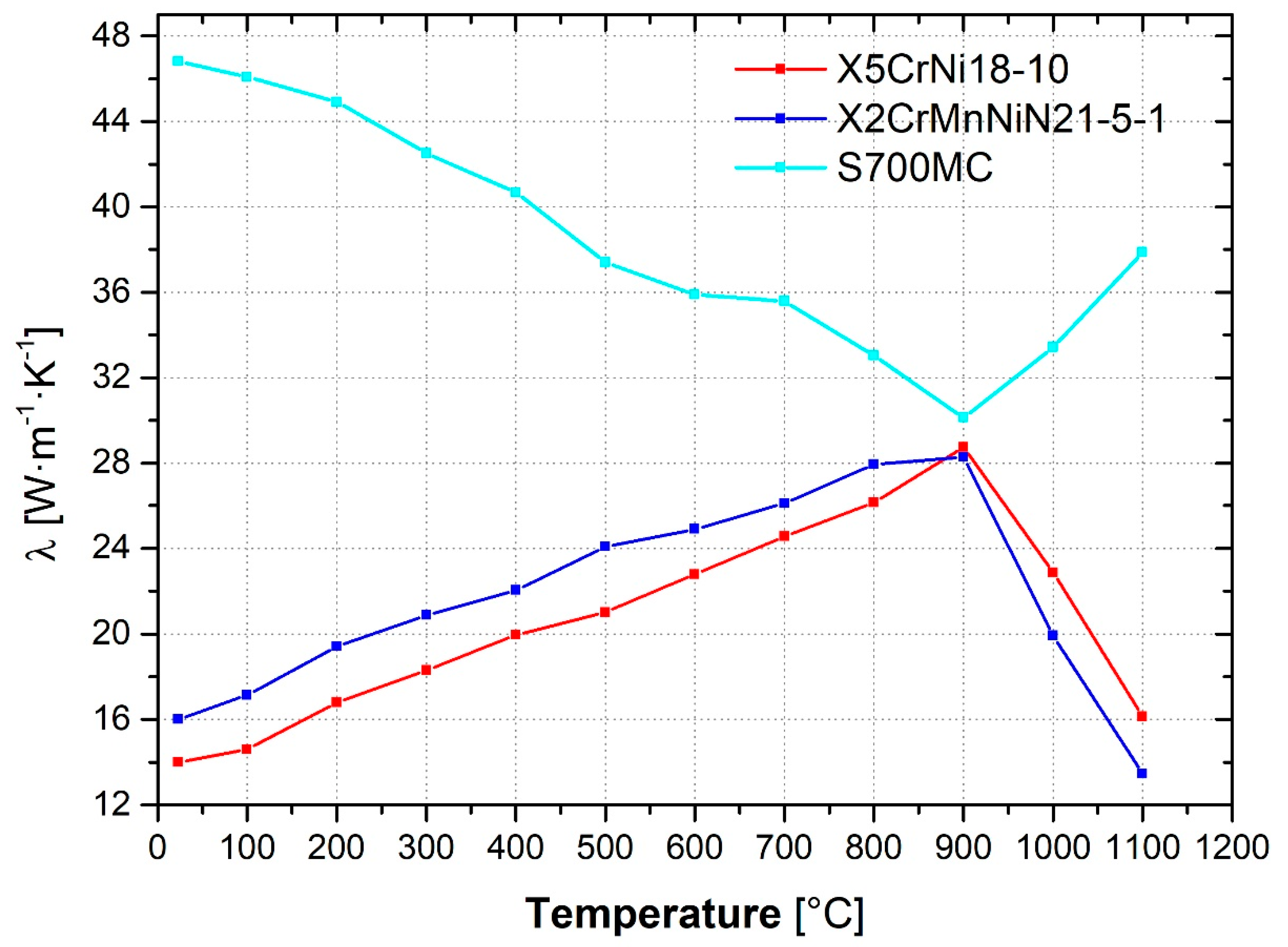
3.2. Determination of the Thermal-Physical Properties

As was already mentioned in the Introduction Section, austenitic steels have higher values of the linear thermal expansion coefficient and lower values of the thermal conductivity compared to the common structural steels, which is why they deform much more during welding. Due to this, not only the values of the linear thermal expansion, α, were measured, but also the values of the thermal conductivity, λ, and thermal diffusivity, a, as well as the values of the specific heat capacity, c. All thermal quantities were measured in the temperature range RT–1100 °C, with a temperature step of 100 °C. Measured values for steel X5CrNi18-10 are shown in Table 3. A graphical comparison of the linear thermal expansion coefficient, α, and the thermal conductivity coefficient, λ, of steel X5CrNi18-10, duplex steel X2CrMnNiN21-5-1, and HSLA steel S700MC is shown in Figure 4 and Figure 5.

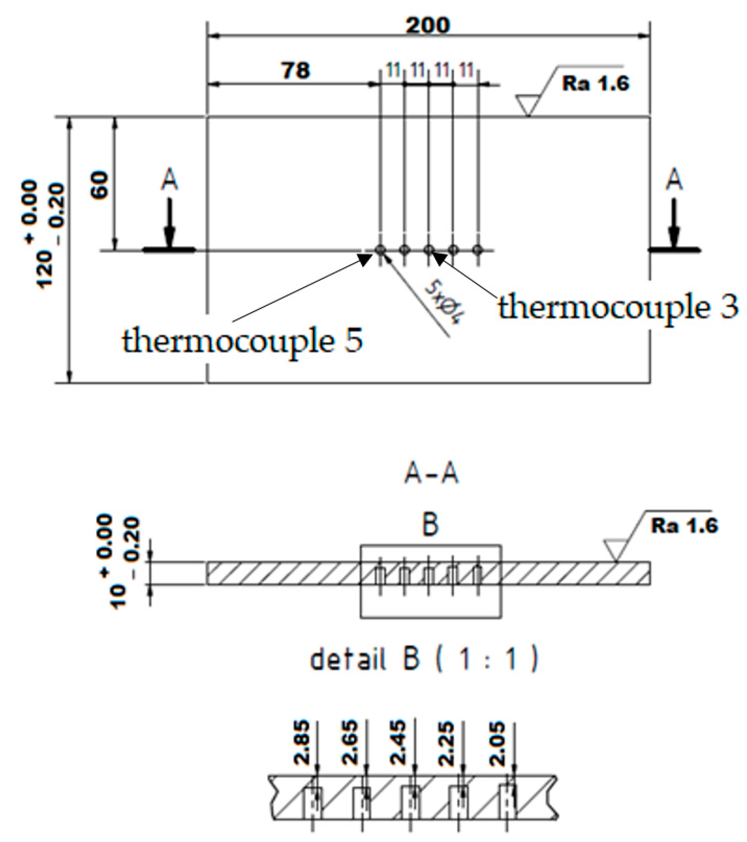
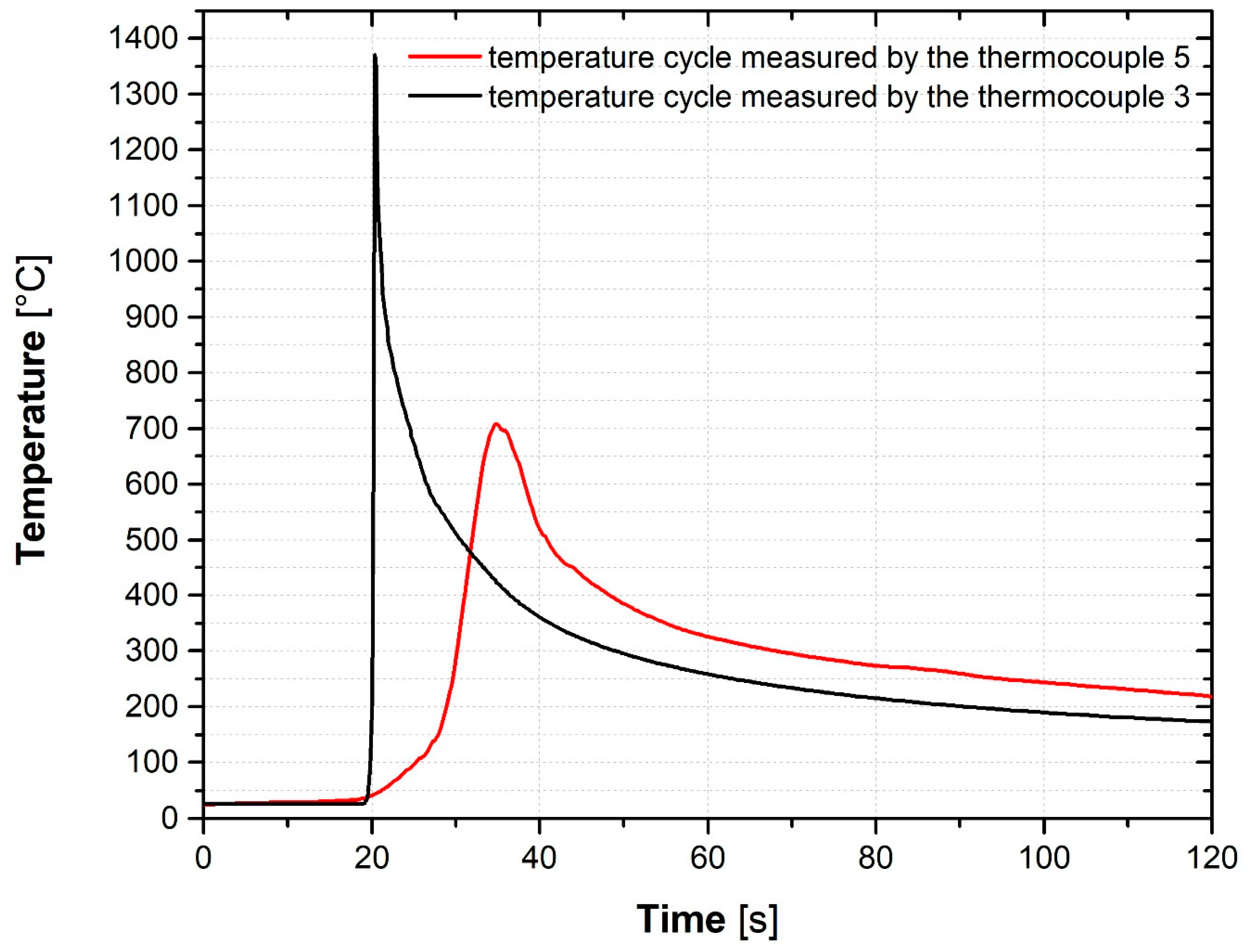
3.3. Measurement of the Temperature Cycles at Real Welding

For physical simulations of the processes that take place in the HAZ of the weld, it is very necessary to arise from the real welding conditions. It is therefore needed to obtain the course of the temperature cycle very close to the fusion line and another temperature cycle from the supposed end of the HAZ. It is very difficult to obtain temperature cycle courses very close to the fusion line, just because of the thermocouple location accuracy. For this reason and based upon experience from the experiments performed on duplex steel [27], an experiment was prepared to monitor the temperature fields in the HAZ. Therefore, as it is shown in Figure 6, a special testing plate was prepared. In the lower part of this plate were milled holes with a diameter of 4 mm, and their depth was changed from each other by 0.2 mm regarding the expected depth of weld penetration. S-type thermocouples were welded into the holes and TIG welding was performed on the surface. During welding, the following effective values of the process parameters were recorded by the WeldMonitor system: I = 152.6 A, U = 21.7 V, travel speed vs. = 3.35 mm·s−1, and the total heat input value was Q = 9.88 kJ·cm−1.
Thermocouples placed in the first two holes were overflowed, as in the case of [27], with a weld pool. The maximum measured temperature was 1512 °C. Thermocouple 3, which was located in the third hole, recorded a temperature cycle with a maximum temperature of 1371 °C. After metallographic evaluation, it appeared that this thermocouple measured a temperature cycle at a distance of 0.07 mm from the fusion line, so this cycle could be used with sufficient accuracy for the physical simulations of processes occurring in the HAZ. Thermocouple 5 measured a temperature cycle with a maximum temperature of 713 °C. Temperatures measured by these two thermocouples (3 and 5—placed in the third and fifth holes) are shown in Figure 7.

3.4. Physical Simulation of the Temperature Cycles in HAZ-Steel X5CrNi18-10

Due to the significant deformation during welding the austenitic steels, these steels are welded with sufficiently rigid clamping, if it is possible. Due to this, the test sample was therefore fixed in the thermo-mechanical simulator Gleeble 3500 so that it could not move when tensile or compressive stresses were applied. Such fixation of the test sample’s position was monitored by a length gauge. Application of the temperature cycle thus induced a stress increase in the sample, which was subsequently compensated by the plastic deformation in the areas of the highest temperatures. This resulted in the residual stresses in the temperature gradient direction. However, it should be noted that compensation of the resulting stresses occurs only in the narrow part of the sample between the high-temperature grips—in the areas of the highest temperatures.

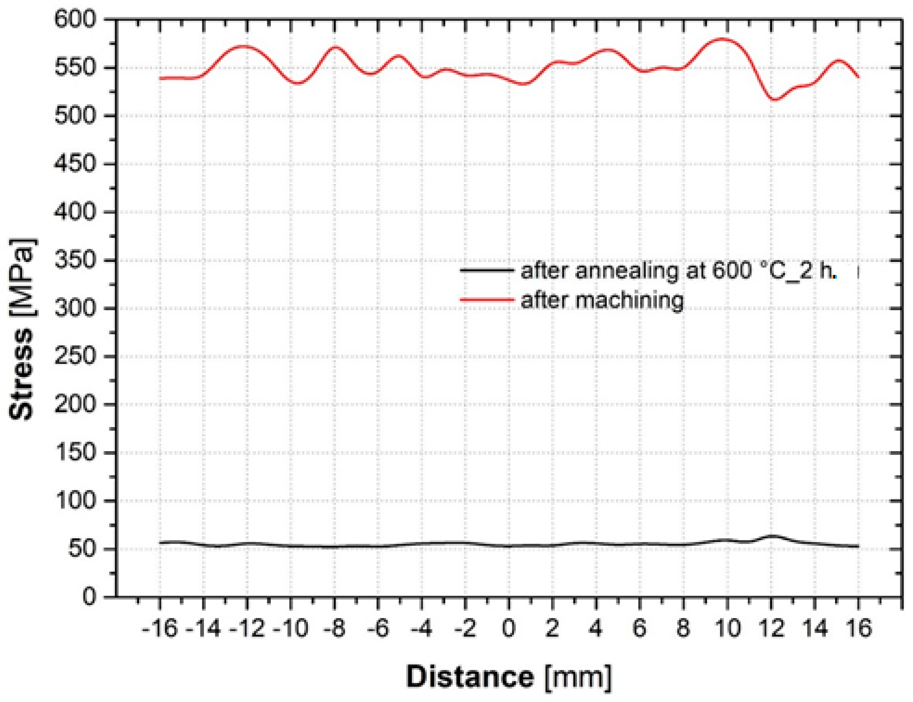
3.5. Analysis of the Residual Stresses via XRD Method

Results of the residual stresses’ analysis after machining of samples and subsequent annealing in the vacuum furnace Reetz are shown in Figure 8. From this graph, it is obvious that machining of samples caused significant tensile stresses in their surface layers. The residual stresses after machining varied by about 550 MPa. By testing the annealing temperatures, it was found that at 600 °C, the residual stresses in the surface layer were reduced by up to 50 MPa, while relatively maintaining the mechanical properties (see Table 2). All test samples were prepared in this way.
Moreover, it was also necessary to assess the repeatability of temperature cycle application in the physical simulations in the thermo-mechanical simulator Gleeble 3500. Therefore, the temperature cycle was firstly applied to six test samples in the Gleeble 3500 device at identical boundary conditions. Courses of the residual stresses, determined by the XRD method for all six samples, are shown in Figure 9.
From Figure 9, it can be seen that the courses of the determined residual stresses were almost identical. There were compressive stresses across the whole HAZ. At the point of reaching the highest temperatures, such compressive residual stresses were about 200 MPa, and at the maximal stress level at a distance of ±6 mm from the sample center, the compressive stresses were about 650 MPa. Samples that were affected by the temperature cycle in the Gleeble 3500 simulator were used to assess the effect of the annealing temperature used above. The samples were subjected to annealing in a vacuum furnace to reduce residual stresses at 450, 500, 550, 600, and 650 °C—every time for 2 h. Results of the residual stress courses after the application of such thermal treatment are shown in Figure 10.

3.6. Hardness Measurement and Structure Study (Temperature Cycle Application)

The sample to which the temperature cycle was applied in the Gleeble 3500 device was metallographically prepared and then hardness was measured according to Vickers HV10. Hardness was measured from the sample center, with individual indentations spaced 0.5 mm apart. The resulting hardness of the basic material was 306 ± 5 HV, and for the material annealed at 600 °C for 2 h it was 307 ± 6 HV. These hardness values were taken as the average of 10 measurements. The final hardness measurements for the samples with residual stresses are (together with a course of these stresses) shown in Figure 11. From the graph, it is clear that the hardness of the structure changed in the same areas as changes in residual stresses. For comparison, Figure 11. also shows a course of the residual stresses after the temperature cycle and subsequent thermal treatment with the relevant hardness values.
Structural and EBSD analyses were performed on the supplied basic material and the material annealed in a vacuum furnace at 600 °C for 2 h. Results of these analyses are shown in Figure 12 and Figure 13. The mean grain size was also measured. The mean grain size of the supplied material was 14.11 ± 12.32 µm, and after annealing at 600 °C, the grain coarsened up to the mean grain size of 22.41 ± 18.45 µm.
Analysis was performed in the same manner for samples where the temperature cycle was applied and for samples where the temperature cycle and subsequent annealing at 600 °C for 2 h were applied. Structural and EBSD analysis was performed at two sample locations depending on the residual stresses’ course. The first analyzed region was in the sample center, and thus the location with the highest temperature and probably the largest plastic deformation (see Figure 14). In addition to that, the location corresponding to the stress peak was analyzed as well (see Figure 15). In the middle of the sample, due to the extensive plastic deformation, recrystallization occurred, and a uniform fine-grained structure was achieved. The mean grain size was found to be 13.56 ± 6.53 µm for samples subjected to the temperature cycle and 14.83 ± 6.30 µm for samples subjected to the temperature cycle and annealing at 600 °C for 2 h. A coarse-grained structure remained in the area of the stress peak with a mean grain size of 21.52 ± 17.11 µm for unannealed samples and 25.54 ± 20.49 µm for the samples where stress-relief annealing was applied. Moreover, the directional orientation of the grains was also evident in this case.

4. Discussion

Physical simulations, which are carried out in the thermal–mechanical simulators, show the possibilities of a detailed investigation of changes that occur during welding in the HAZ. By using the thermal–mechanical simulator Gleeble 3500, there can be conditions prepared that correspond to the real welding, and it also ensures their repeatability. However, the biggest advantage of these simulations is the study of HAZ on a larger scale. At real welding, an HAZ width of only 0.8 mm was determined. Using physical simulations, that area was enlarged approximately 6.5 times and thus studies could be performed on an area having a length of 5.2 mm. Such an increase of the HAZ is a necessity when analyzing residual stresses using X-ray diffraction because otherwise, individual measurements would overlap each other. Even when focusing the beam with a 0.5 mm collimator, only two measurements would fit into a real HAZ. With the physical simulations, approximately six or seven measurements can be placed in the enlarged HAZ. The same is true for the structural evaluation of the HAZ sub-regions.
XRD analyses are one of the already established NDT methods for determining the residual stresses. On the other hand, their great disadvantage is their significant sensitivity to the influence of technological processing on the surface of tested samples. This disadvantage can be partially eliminated by etching of the hardened surface, but there are still some limitations on the size of the etched area. Although physical simulations make it possible to carry out detailed studies of the processes occurring in HAZ, they also require that relevant studies should be carried out on areas from 70 to 320 mm2, which was almost impossible in light of the uniform etching of the tested surface. Therefore, prior to the actual application of the temperature cycles, an annealing was applied (see Figure 8) to reduce the residual stresses to acceptable initial values (stress-relief annealing). This, together with the conditions set in the thermo-mechanical simulator, can ensure a very high repeatability degree of the performed experiments, and therefore extend the range of the subsequent operations.
From Figure 9, it is obvious that in the case of six samples subjected to the same temperature cycle and with the same boundary conditions, identical residual stress distributions across the HAZ were obtained. In addition to that, magnitudes of the residual stresses were also very similar. Slightly larger differences in values can be found in the area of the stress peaks. However, here, the differences did not exceed 11%.
In summary, the occurrence of the residual stresses in steel parts is arising from the interaction effects of restrained volume expansion during local heating and restrained shrinkage during cooling. For welded joints of the structural steels, significant compressive stress peaks occur at larger distances from the fusion line (i.e., outside the HAZ). These stresses start to transform into tensile ones in the HAZ, with a certain decrease of tensile stresses in the area of maximum temperatures, which is verified by the results obtained from physical simulations of ferritic-pearlite [26] or from the other studies [13,18,33,34,35]. Exactly the same shape and distribution of the residual stresses were also obtained from physical simulations of welding with duplex steel X2CrMnNiN21-5-1 [27], only all residual stresses were compressive ones. Moreover, compressive stresses over the whole analyzed area were also obtained in the case of the austenitic steel X5CrNi18-10. Regarding the duplex steel, the difference was at the area of maximum temperatures.
Figure 16 shows a comparison of the residual stresses’ magnitudes and distribution after physical simulations of the following materials: austenitic steel X5CrNi18-10, duplex steel X2CrMnNiN21-5-1 [27], and HSLA steel S700MC [26]. All experiments were performed with identical conditions (shape and dimensions of samples, clamping method, free length of the working part, etc.). From the measured courses, it is clear that with the same shape of sample and the same width of HAZ, the compressive stress peaks were detected in the same locations, regardless of the material type. However, significant changes in the residual stresses’ distribution and values occurred in the HAZ. For the austenitic steel X5CrNi18-10, a constant compressive stress of 200 MPa was achieved almost throughout the whole HAZ. In the case of duplex steel X2CrMnNiN21-5-1, compressive stresses were also determined throughout the whole HAZ, but the profile was very different. There were significant local minimal values at the edges of HAZ (−600 MPa), and in the middle of the sample, at the area of the highest temperatures, the compressive stress was over 400 MPa. For HSLA steel S700MC, the course of the residual stresses in the HAZ was similar to that of the duplex steel, but the stresses in the HAZ were tensile ones.
The uniformity of residual stresses in the austenitic steel is mainly due to the thermal–physical properties of the material. The high values of the linear and volume thermal expansion coefficients and the low values of the thermal conductivity coefficient caused heat to be dissipated from the sample center more slowly, resulting in intense plastic deformation. This resulted in restoration and recrystallization in the HAZ, as confirmed by the significant reduction of hardness from 295 to 175 HV10 and by the reduction, and mainly by the more uniform distribution of the mean grain size—its magnitudes decreased from 22.41 ± 18.45 to 13.56 ± 6.53 µm.
Application of the temperature cycles to the sample during rigid clamping influenced not only the structural properties (grain size), but also the mechanical properties. In the case of the supplied, strain-hardened basic material, the mean grain size was 14.11 ± 12.32 µm. Yield strength was 803.1 ± 5.2 MPa and UTS = 853.1 ± 4.8 MPa. Annealing of the samples at 600 °C for 2 h resulted in grain coarsening and higher heterogeneity in the grain size—up to 22.41 ± 18.45 µm. Simultaneously, there was a decrease in the yield strength to 715.9 ± 4.2 MPa and a slight decrease in the UTS to 844.6 ± 6.4 MPa. The expected decrease in the yield strength was caused by the restoration processes during the annealing. What is interesting, however, is the intensive increase in the mean grain size as well as the increase in the grain heterogeneity given by the standard deviation at relatively low annealing temperatures.
By applying the temperature cycle, grains in the HAZ were refined and revealed more uniform distribution, as described above. On the other hand, there was a significant reduction in hardness and especially YS and UTS. The value of YS decreased in this area to 356.3 ± 3.7, and in the case of UTS to 637.5 ± 4.8 MPa. At the area of the maximal stress peaks, the mean grain size remained similar to that of the annealed material, and only a slight increase in hardness HV10 occurred.
The subsequent application of stress-relief annealing did not lead to further changes in the mechanical properties. There was only a slight increase in the mean grain size, especially in the area of stress peaks from 21.52 ± 17.11 up to 25.54 ± 20.49 µm.

5. Conclusions

The major aim of the study presented in this paper was to assess the possibility of using physical simulations in monitoring the residual stresses’ distribution in the HAZ of the austenitic steel welds, as well as to assess the results achieved with similar studies performed on the HSLA and duplex steel. Obtained results can be summarized in the following points:
(1)
With the help of the physical simulations, it is possible to study, in detail, processes that occur in the HAZ during application of the thermal–mechanical cycles. Due to the proposed methodology, HAZ can be extended up to a 6.5 times larger area, which enables a more detailed assessment of the sub-areas both in light of the residual stresses and from the structural analyses point of view. However, it should be remembered that this is only a simulation of real processes.
(2)
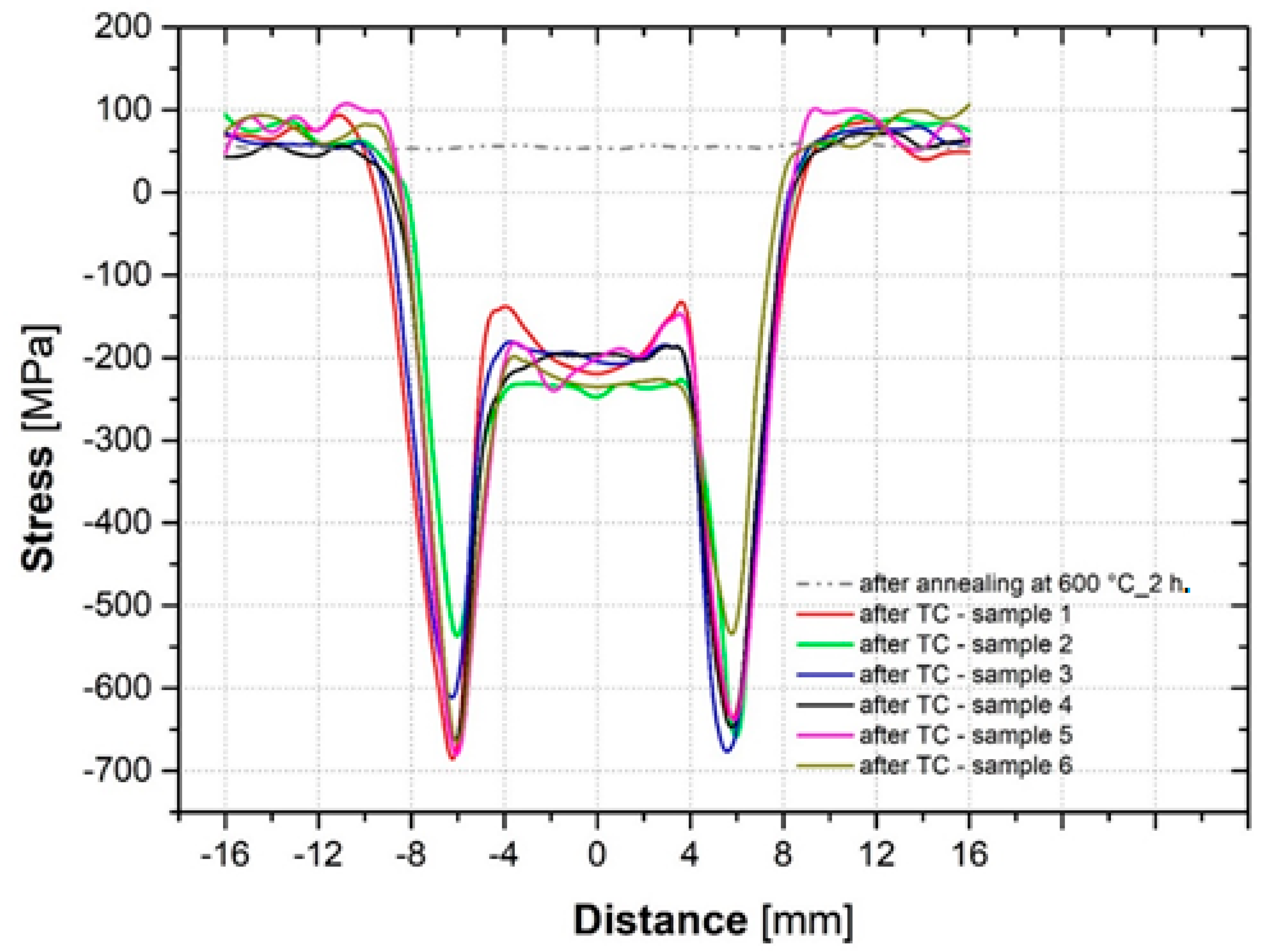
As part of the submitted research, it was possible to prove the functionality and, above all, the repeatability of the proposed methodology while maintaining the boundary conditions. From the performed analyses (carried out on six samples), a high agreement both in the distribution and magnitude of the residual stresses was evident.
(3)
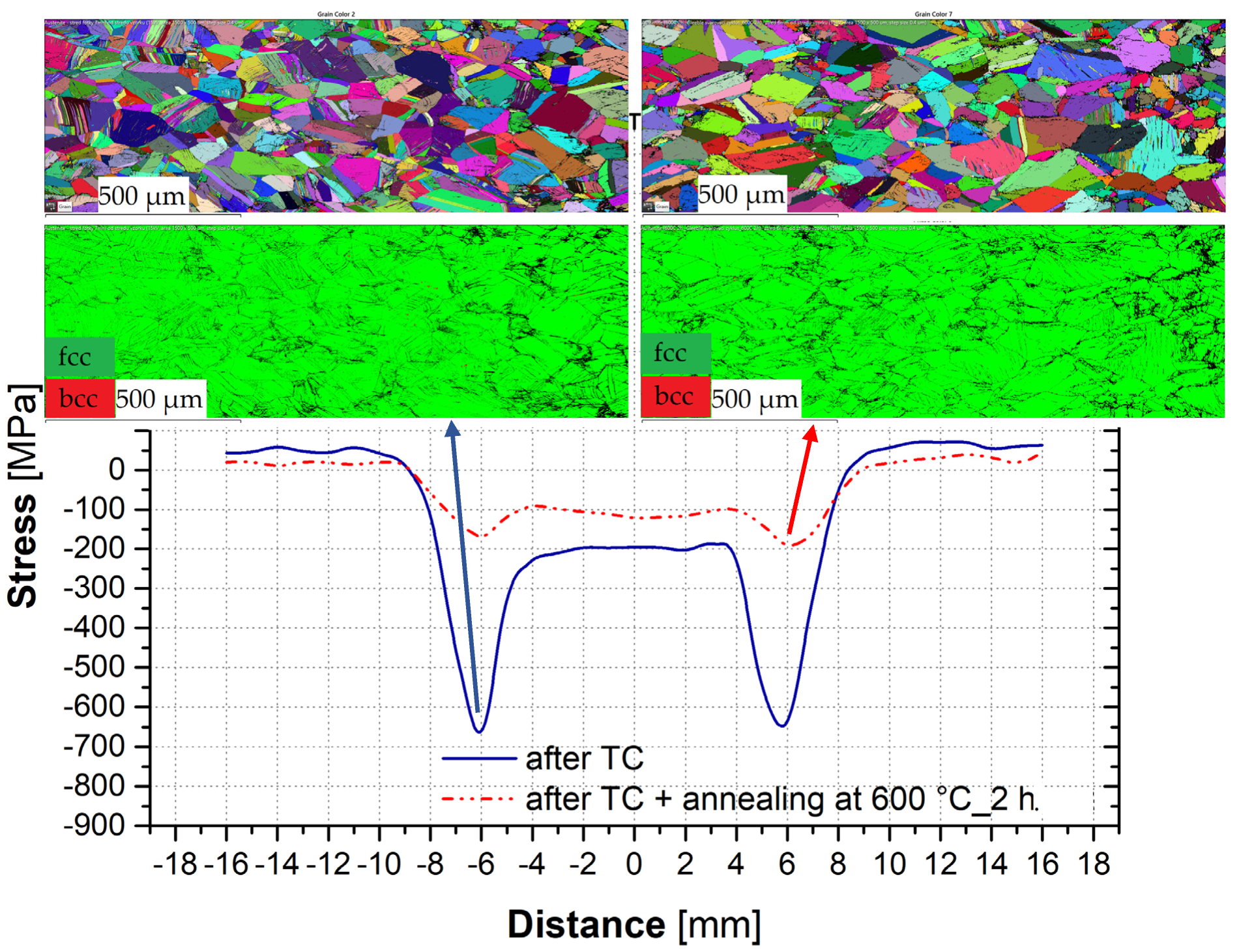
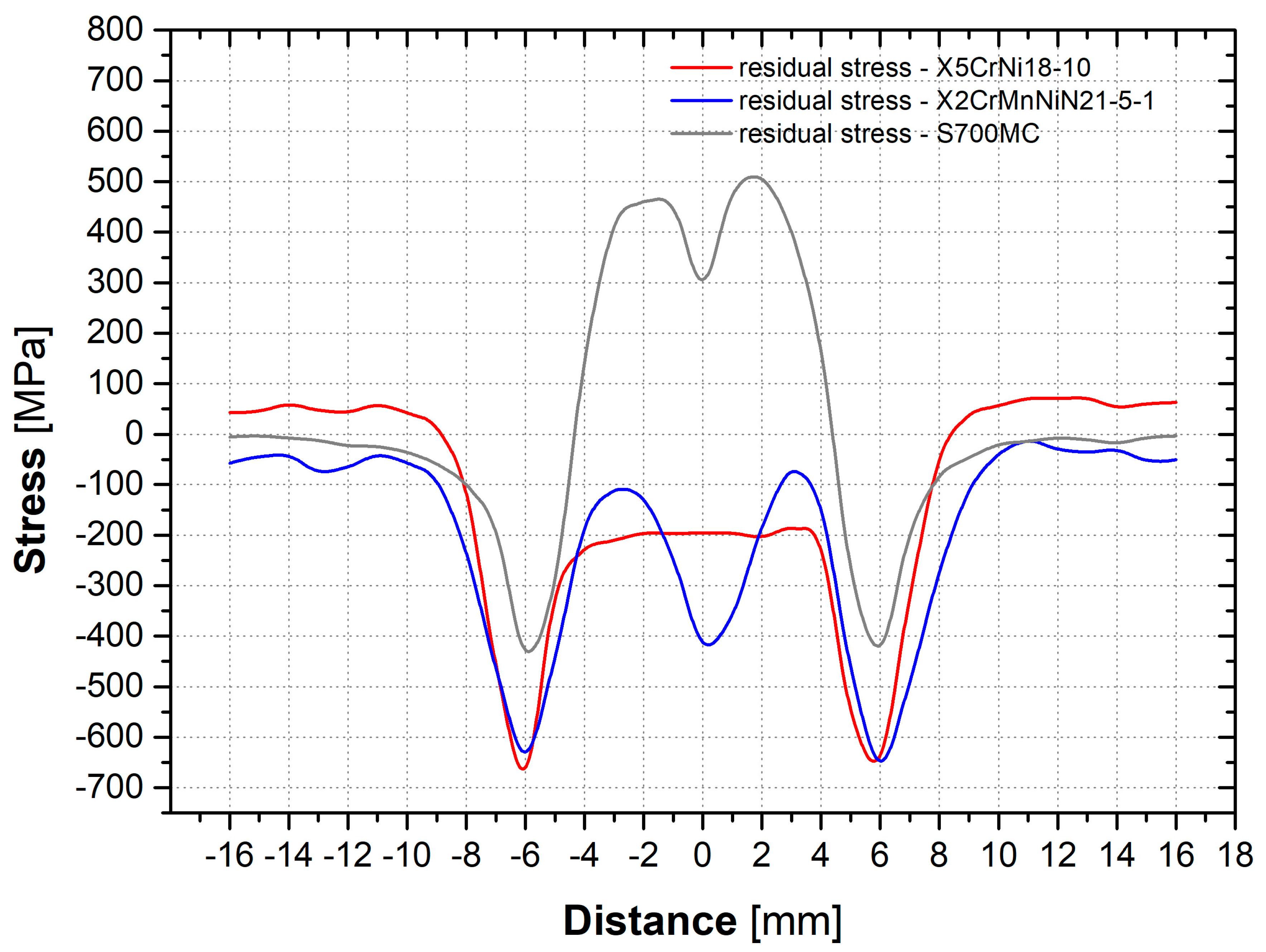
Analysis of the residual stresses after application of the temperature cycles, determined by the XRD method, detected the local stress peaks outside the HAZ, as in the case of duplex and HSLA steels. In the HAZ, however, the course of the residual stresses was different for the austenitic steel X5CrNi18-10. The reason rests primarily in the different material properties—thermal conductivity and volume thermal expansion.
(4)
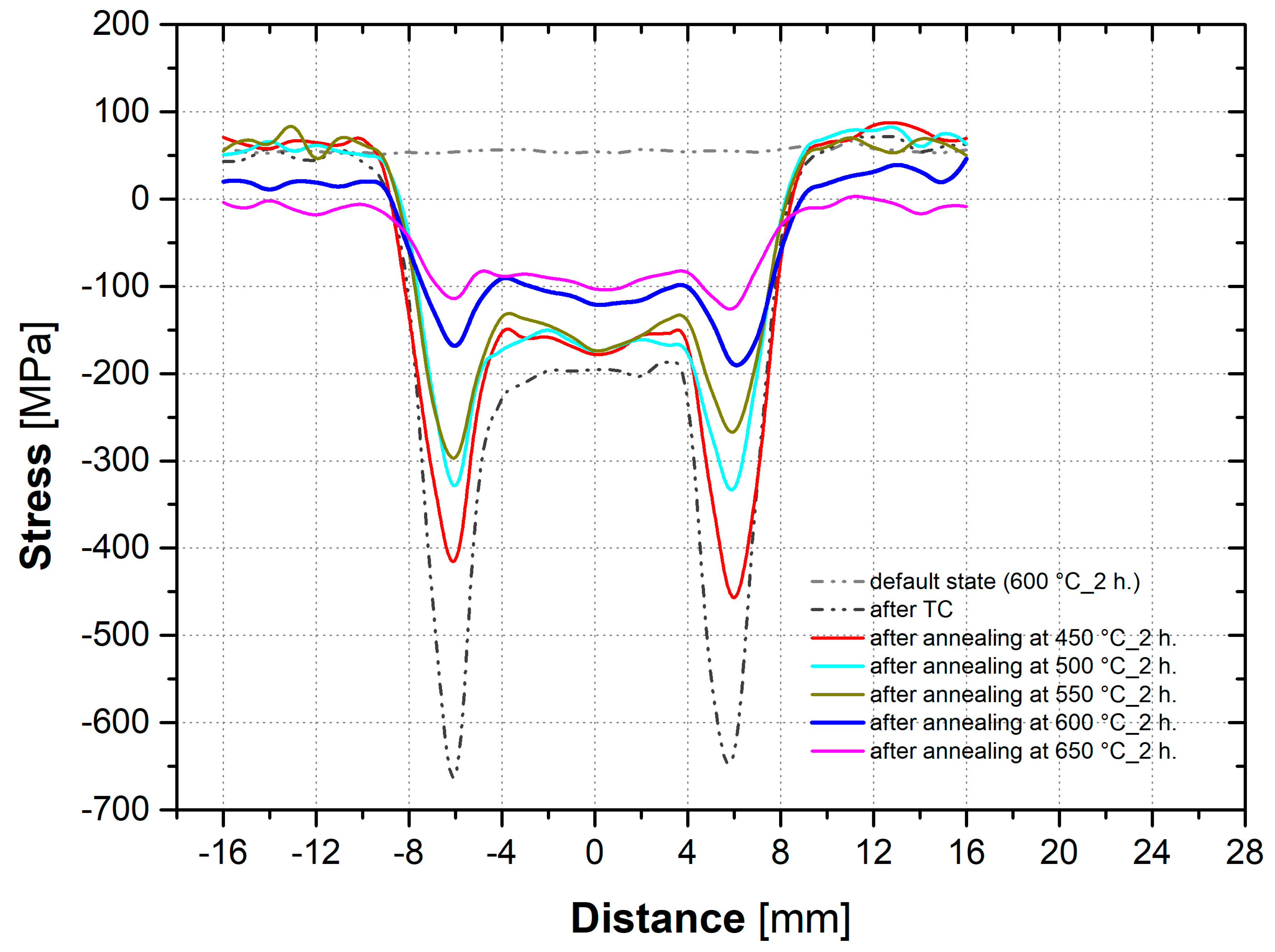
Detected stress peaks can be eliminated by the stress-relief annealing to reduce residual stresses. As the PWHT temperature increased, the size of the stress peaks decreased, and during annealing (T = 650 °C, t = 2 h), the stress peaks were removed completely. Compressive residual stresses of approximately 100 MPa remained in the tested material.
(5)
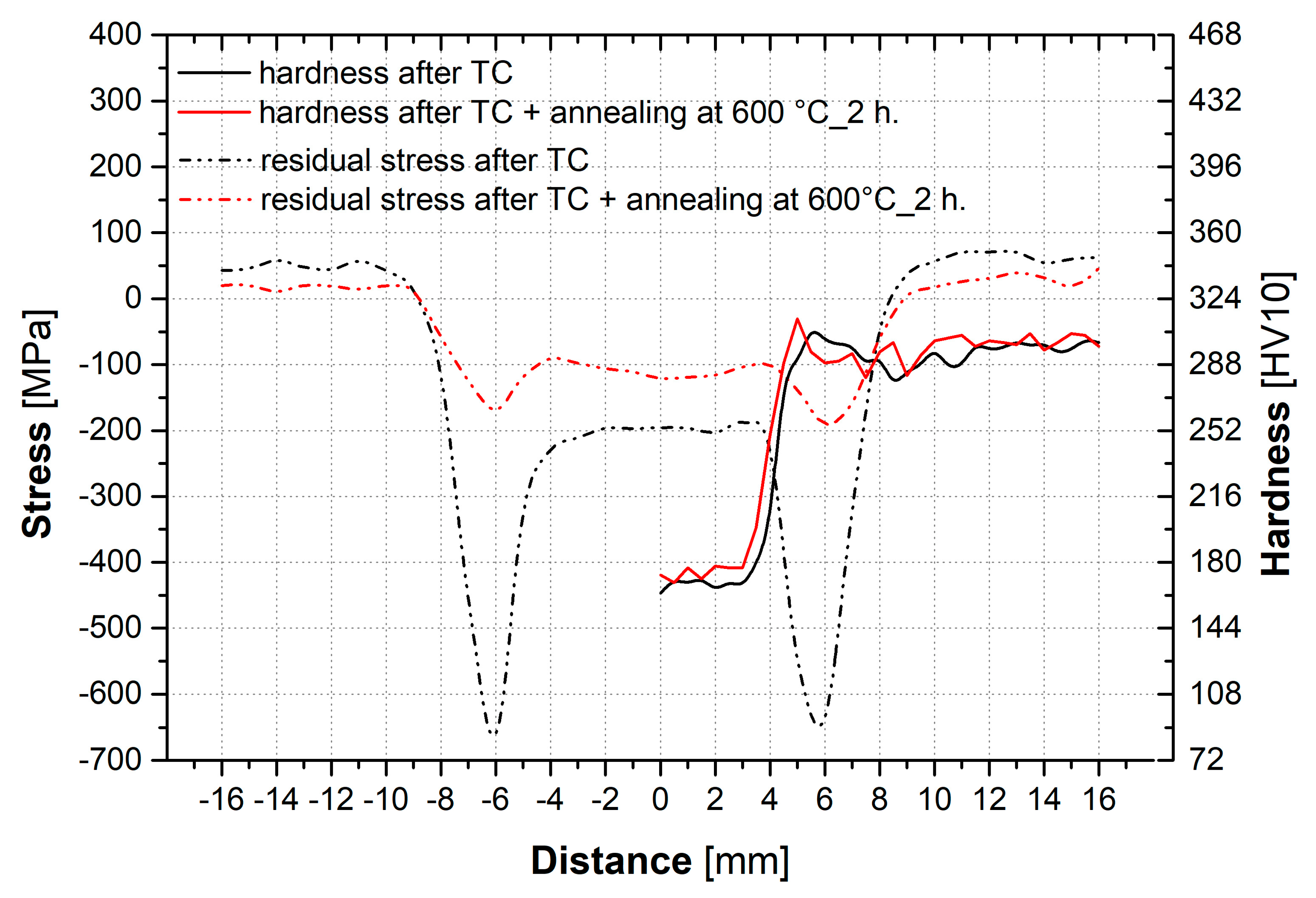
Application of the temperature cycles resulted in a significant reduction of mechanical properties and hardness in the HAZ. YS decreased by 49%, UTS by 24%, and hardness HV10 by 41%. Subsequent stress-relief annealing (T = 600 °C, t = 2 h) had only a minimal effect on the mechanical properties.
(6)
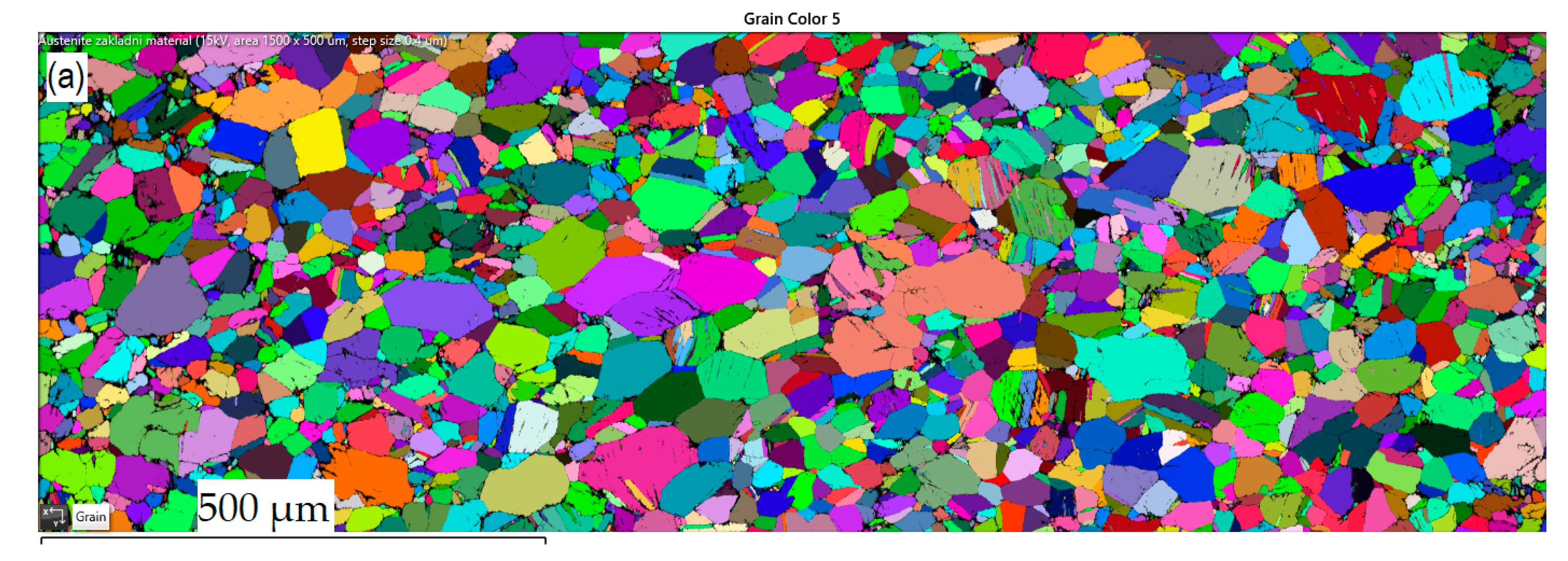
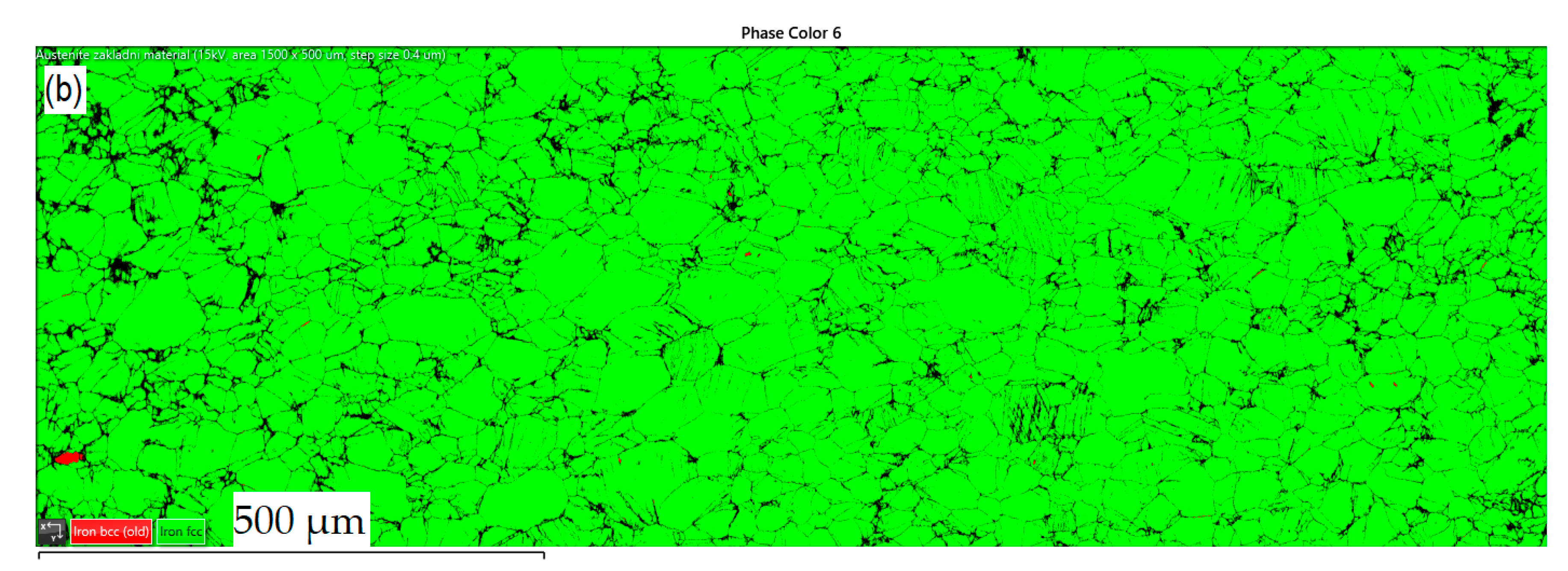
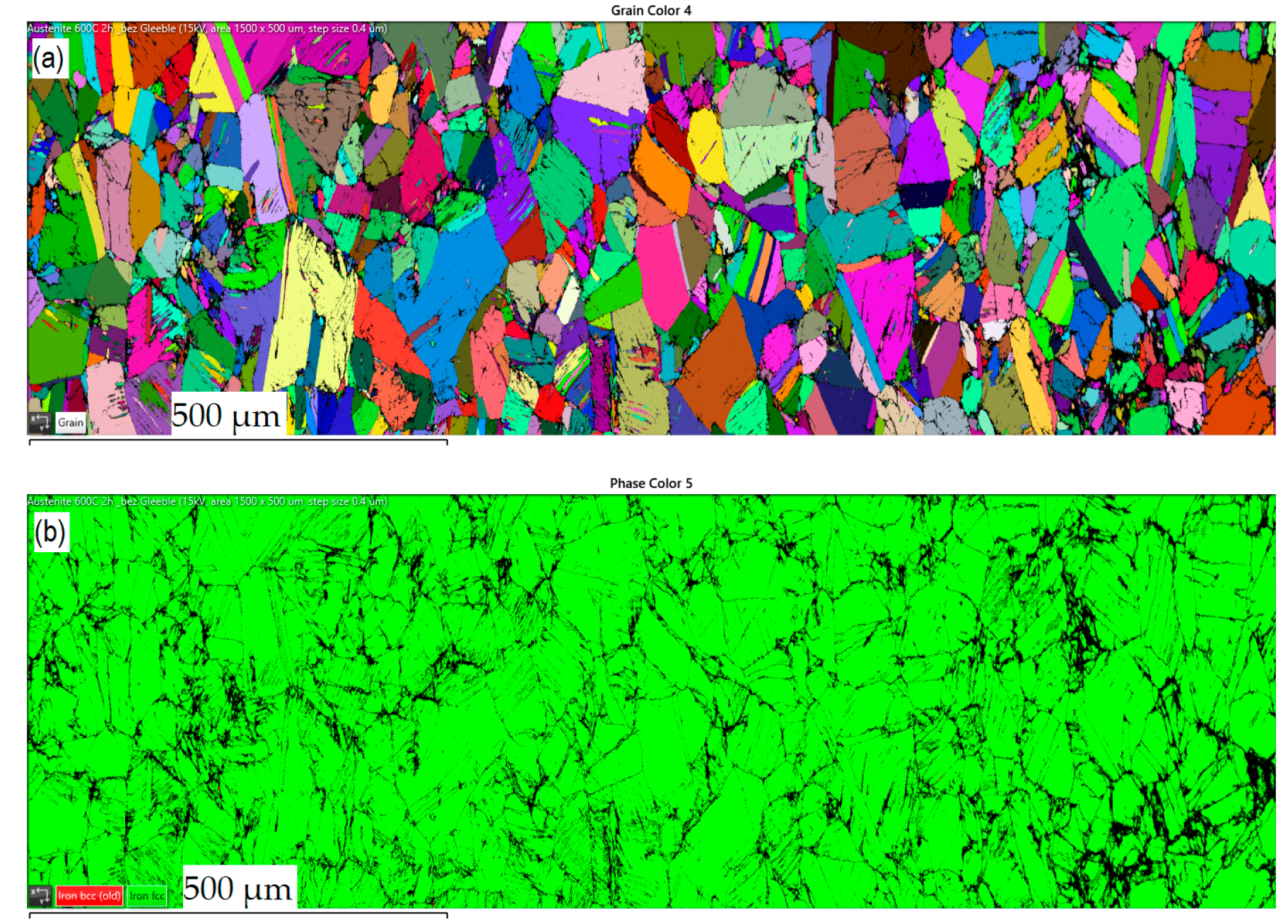
Applied thermal–mechanical cycles as well as the annealing used affected the grain size. Annealing at 600 °C for 2 h caused a grain coarsening by about 60%. By applying the temperature cycles (together with the rigid clamping and subsequent plastic deformation), the grain was refined and had more uniform distribution in the HAZ. Compared to the annealed state (Figure 13), the mean grain size decreased by 40%. However, at the same time, there was an intense strain hardening of the material and thus a decrease in YS.

Author Contributions

Conceptualization, J.M. and Š.B.; methodology, M.Š.; investigation, Š.B., J.M. and M.Š.; resources, J.M. and Š.B.; data curation, M.Š. and Š.B.; writing—original draft preparation, Š.B.; writing—review and editing, J.M., M.Š. and J.S.; visualization, Š.B.; supervision, J.M.; funding acquisition, Š.B. All authors have read and agreed to the published version of the manuscript.

Funding

This research was funded by the Student Grant Competition of the Technical University of Liberec under the project No. SGS-2020-5008: “Influence of residual stresses during technological processing on fatigue life of manufactured parts”.

Institutional Review Board Statement

Not applicable.

Informed Consent Statement

Not applicable.

Data Availability Statement

Not applicable.

Conflicts of Interest

The authors declare no conflict of interest.

References

  1. Jandera, M.; Machacek, J. Residual Stresses and Strength of Hollow Stainless Steel Sections. 2007, pp. 262–263. Available online: https://www.researchgate.net/publication/268358021 (accessed on 29 September 2022).
  2. Elmesalamy, A.; Francis, J.A.; Li, L. A Comparison of Residual Stresses in Multi Pass Narrow Gap Laser Welds and Gas-Tungsten Arc Welds in AISI 316L Stainless Steel. Int. J. Press. Vessel. Pip. 2014, 113, 49–59. [Google Scholar] [CrossRef]
  3. Outeiro, J.; Pina, J.; M’saoubi, R.; Pusavec, F.; Jawahir, I. Analysis of Residual Stresses Induced by Dry Turning of Difficult-to-Machine Materials. CIRP Ann. 2008, 57, 77–80. [Google Scholar] [CrossRef] [Green Version]
  4. Bozga, M.-B.; Popa, M.S.; Sattel, S.; Tomoiagă, V.-B. Influence of the Cutting Edge Microgeometry on the Tool Life in Austenitic Stainless Steel Machining with Carbide End Mill; EDP Sciences: Les Ulis, France, 2017; Volume 112, p. 01016. [Google Scholar]
  5. Dubovska, R.; Majerik, J.; Čep, R.; Kouřil, K. Investigating the Influence of Cutting Speed on the Tool Life of a Cutting Insert While Cutting DIN 1.4301 Steel. Mater. Technol. 2016, 50, 439–445. [Google Scholar] [CrossRef]
  6. Kolařík, L.; Kolaříková, M.; Novák, P.; Sahul, M.; Vondrouš, P. The Influence of Nickel Interlayer for Diffusion Welding of Titanium and Austenitic Stainess Steel; Metal: Brno, Czech Republic, 2013. [Google Scholar]
  7. Lee, C.-H.; Chang, K.-H. Comparative Study on Girth Weld-Induced Residual Stresses between Austenitic and Duplex Stainless Steel Pipe Welds. Appl. Therm. Eng. 2014, 63, 140–150. [Google Scholar] [CrossRef]
  8. Dakhlaoui, R.; Braham, C.; Baczmański, A. Mechanical Properties of Phases in Austeno-Ferritic Duplex Stainless Steel—Surface Stresses Studied by X-ray Diffraction. Mater. Sci. Eng. A 2007, 444, 6–17. [Google Scholar] [CrossRef]
  9. Johansson, J.; Odén, M. Load Sharing between Austenite and Ferrite in a Duplex Stainless Steel during Cyclic Loading. Metall. Mater. Trans. A 2000, 31, 1557–1570. [Google Scholar] [CrossRef]
  10. Wei, H.; Chen, Y.; Yu, W.; Su, L.; Wang, L.; Tang, D. Determination of the Macroscopic Residual Stress: Modeling and Experimental Evaluation of Texture and Local Grain-Interaction. Mater. Charact. 2020, 169, 110609. [Google Scholar] [CrossRef]
  11. Zhang, X.X.; Ni, D.R.; Xiao, B.L.; Andrä, H.; Gan, W.M.; Hofmann, M.; Ma, Z.Y. Determination of Macroscopic and Microscopic Residual Stresses in Friction Stir Welded Metal Matrix Composites via Neutron Diffraction. Acta Mater. 2015, 87, 161–173. [Google Scholar] [CrossRef]
  12. Jang, D.; Watkins, T.; Kozaczek, K.; Hubbard, C.; Cavin, O. Surface Residual Stresses in Machined Austenitic Stainless Steel. Wear 1996, 194, 168–173. [Google Scholar] [CrossRef]
  13. Ragavendran, M.; Vasudevan, M.; Hussain, N. Study of the Microstructure, Mechanical Properties, Residual Stresses, and Distortion in Type 316LN Stainless Steel Medium Thickness Plate Weld Joints. J. Mater. Eng. Perform. 2022, 31, 5013–5025. [Google Scholar] [CrossRef]
  14. Monin, V.I.; Lopes, R.T.; Turibus, S.N.; Payão Filho, J.C.; de Assis, J.T. X-ray Diffraction Technique Applied to Study of Residual Stresses after Welding of Duplex Stainless Steel Plates. Mater. Res. 2014, 17, 64–69. [Google Scholar] [CrossRef] [Green Version]
  15. Ouali, N.; Khenfer, K.; Belkessa, B.; Fajoui, J.; Cheniti, B.; Idir, B.; Branchu, S. Effect of Heat Input on Microstructure, Residual Stress, and Corrosion Resistance of UNS 32101 Lean Duplex Stainless Steel Weld Joints. J. Mater. Eng. Perform. 2019, 28, 4252–4264. [Google Scholar] [CrossRef]
  16. Mcirdi, L.; Inal, K.; Lebrun, J. Analysis by X-Ray Diffraction of the Mechanical Behaviour of Austenitic and Ferritic Phases of a Duplex Stainless Steel. Adv. X-ray Anal. 2000, 42, 397–406. [Google Scholar]
  17. Johansson, J. Residual Stresses and Fatigue in a Duplex Stainless Steel. Licentiate Thesis, Division of Engineering Materials, Departement of Mechanical Engineering, Linköpings Universitet, Linköping, Sweden, 1999. [Google Scholar]
  18. Alipooramirabad, H.; Paradowska, A.; Ghomashchi, R.; Reid, M. Investigating the Effects of Welding Process on Residual Stresses, Microstructure and Mechanical Properties in HSLA Steel Welds. J. Manuf. Process. 2017, 28, 70–81. [Google Scholar] [CrossRef]
  19. Banik, S.D.; Kumar, S.; Singh, P.K.; Bhattacharya, S.; Mahapatra, M.M. Distortion and Residual Stresses in Thick Plate Weld Joint of Austenitic Stainless Steel: Experiments and Analysis. J. Mater. Process. Technol. 2021, 289, 116944. [Google Scholar] [CrossRef]
  20. Magnier, A.; Zinn, W.; Niendorf, T.; Scholtes, B. Residual Stress Analysis on Thin Metal Sheets Using the Incremental Hole Drilling Method–Fundamentals and Validation. Exp. Technol. 2019, 43, 65–79. [Google Scholar] [CrossRef]
  21. Payares-Asprino, C.; Muñoz-Escalona, P.; Sanchez, A. Residual Stress in Machined Duplex Stainless Steel Welds Developed through Automatic Process; Pontificia Universidad Católica del Perú: Lima, Peru, 2019; pp. 222–230. [Google Scholar]
  22. Jiménez, C.A.V.; Rosas, G.G.; González, C.R.; Alejo, V.G.; Hereñú, S. Effect of Laser Shock Processing on Fatigue Life of 2205 Duplex Stainless Steel Notched Specimens. Opt. Laser Technol. 2017, 97, 308–315. [Google Scholar] [CrossRef]
  23. Wan, Y.; Jiang, W.; Song, M.; Huang, Y.; Li, J.; Sun, G.; Shi, Y.; Zhai, X.; Zhao, X.; Ren, L. Distribution and Formation Mechanism of Residual Stress in Duplex Stainless Steel Weld Joint by Neutron Diffraction and Electron Backscatter Diffraction. Mater. Des. 2019, 181, 108086. [Google Scholar] [CrossRef]
  24. Brown, D.; Bernardin, J.; Carpenter, J.; Clausen, B.; Spernjak, D.; Thompson, J. Neutron Diffraction Measurements of Residual Stress in Additively Manufactured Stainless Steel. Mater. Sci. Eng. A 2016, 678, 291–298. [Google Scholar] [CrossRef] [Green Version]
  25. Yuan, H.; Wang, Y.; Shi, Y.; Gardner, L. Residual Stress Distributions in Welded Stainless Steel Sections. Thin-Walled Struct. 2014, 79, 38–51. [Google Scholar] [CrossRef] [Green Version]
  26. Kik, T.; Moravec, J.; Švec, M. Experiments and Numerical Simulations of the Annealing Temperature Influence on the Residual Stresses Level in S700MC Steel Welded Elements. Materials 2020, 13, 5289. [Google Scholar] [CrossRef]
  27. Moravec, J.; Bukovská, Š.; Švec, M.; Sobotka, J. Possibilities to Use Physical Simulations When Studying the Distribution of Residual Stresses in the HAZ of Duplex Steels Welds. Materials 2021, 14, 6791. [Google Scholar] [CrossRef]
  28. Murugan, S.; Rai, S.K.; Kumar, P.; Jayakumar, T.; Raj, B. Temperature Distribution and Residual Stresses Due to Multipass Welding in Type 304 Stainless Steel and Low Carbon Steel Weld Pads. Int. J. Press. Vessel. Pip. 2001, 78, 307–317. [Google Scholar] [CrossRef]
  29. Vasantharaja, P.; Maduarimuthu, V.; Vasudevan, M.; Palanichamy, P. Assessment of Residual Stresses and Distortion in Stainless Steel Weld Joints. Mater. Manuf. Process. 2012, 27, 1376–1381. [Google Scholar] [CrossRef]
  30. Huang, B.; Liu, J.; Zhang, S.; Chen, Q.; Chen, L. Effect of Post-Weld Heat Treatment on the Residual Stress and Deformation of 20/0Cr18Ni9 Dissimilar Metal Welded Joint by Experiments and Simulations. J. Mater. Res. Technol. 2020, 9, 6186–6200. [Google Scholar] [CrossRef]
  31. Sadeghi, B.; Sharifi, H.; Rafiei, M.; Tayebi, M. Effects of Post Weld Heat Treatment on Residual Stress and Mechanical Properties of GTAW: The Case of Joining A537CL1 Pressure Vessel Steel and A321 Austenitic Stainless Steel. Eng. Fail. Anal. 2018, 94, 396–406. [Google Scholar] [CrossRef]
  32. Zhang, Z.; Ge, P.; Zhao, G. Numerical Studies of Post Weld Heat Treatment on Residual Stresses in Welded Impeller. Int. J. Press. Vessel. Pip. 2017, 153, 1–14. [Google Scholar] [CrossRef]
  33. Pamnani, R.; Sharma, G.K.; Mahadevan, S.; Jayakumar, T.; Vasudevan, M.; Rao, B. Residual Stress Studies on Arc Welding Joints of Naval Steel (DMR-249A). J. Manuf. Process. 2015, 20, 104–111. [Google Scholar] [CrossRef]
  34. Lin, J.; Ma, N.; Lei, Y.; Murakawa, H. Measurement of Residual Stress in Arc Welded Lap Joints by Cosα X-ray Diffraction Method. J. Mater. Process. Technol. 2017, 243, 387–394. [Google Scholar] [CrossRef]
  35. Hensel, J.; Nitschke-Pagel, T.; Dilger, K. On the Effects of Austenite Phase Transformation on Welding Residual Stresses in Non-Load Carrying Longitudinal Welds. Weld. World 2015, 59, 179–190. [Google Scholar] [CrossRef]
Figure 1. Drawing of the sample used for the physical simulation and determination of the residual stresses via the XRD method [27].
Metals 12 01891 g001
Figure 2. Example of the real samples after the temperature cycle—maximal temperature 1386 °C.
Metals 12 01891 g002
Figure 3. Clamping of the tested sample in the Gleeble 3500 device before application of the temperature cycle.
Metals 12 01891 g003
Figure 4. Courses of the linear thermal expansion coefficient in dependence on temperature (X5CrNi18-10, X2CrMnNiN21-5-1, and S700MC).
Metals 12 01891 g004
Figure 5. Courses of the thermal conductivity in dependence on temperature (X5CrNi18-10, X2CrMnNiN21-5-1, and S700MC).
Metals 12 01891 g005
Figure 6. Drawing of the testing plate for determination of the temperature cycles in HAZ [27].
Metals 12 01891 g006
Figure 7. Temperature cycles measured by the thermocouples 3 and 5.
Metals 12 01891 g007
Figure 8. Residual stresses after machining (red curve) and after annealing (black curve).
Metals 12 01891 g008
Figure 9. Courses of the residual stresses after TC for the annealed sample (grey curve), sample 1 (red curve), sample 2 (light green curve), sample 3 (blue curve), sample 4 (black curve), sample 5 (pink curve), and for sample 6 (dark green curve).
Metals 12 01891 g009
Figure 10. Residual stresses after annealing at different temperatures.
Metals 12 01891 g010
Figure 11. Residual stresses and hardness after the temperature cycle and after TC + annealing.
Metals 12 01891 g011
Figure 12. Display of grains (a) and phases (b)—steel X5CrNi18-10 in the basic state.
Metals 12 01891 g012aMetals 12 01891 g012b
Figure 13. Display of grains (a) and phases (b)—steel X5CrNi18-10 in the annealed state (600 °C, 2 h).
Metals 12 01891 g013
Figure 14. Display of grains and phases—steel X5CrNi18-10 after TC in the area of the maximal temperatures with the relevant courses of residual stresses.
Metals 12 01891 g014
Figure 15. Display of grains and phases—steel X5CrNi18-10 after TC in the area of the maximal stresses with the relevant courses of residual stresses.
Metals 12 01891 g015
Figure 16. Courses of the residual stresses after TC for austenitic, duplex [27], and ferrite-pearlite steel S700MC [26].
Metals 12 01891 g016
Table 1. Chemical composition (wt.%) of the steel X5CrNi18-10.
CCrMnNiSiS
EN 10088-1min.-17.00-8.00--
max.<0.0719.502.0010.501.000.015
Experiment 0.04618.381.668.100.230.014
Table 2. Basic mechanical properties of tested materials (basic, annealed, and after TC).
Sample
No.
YS
(MPa)
UTS
(MPa)
Ag
(%)
A80
(%)
BM803.1 ± 5.2853.1 ± 4.83.04 ± 0.4322.84 ± 1.92
A600715.9 ± 4.2844.6 ± 6.714.19 ± 1.1627.15 ± 1.24
TC1371356.3 ± 3.7637.5 ± 4.87.88 ± 0.6512.66 ± 1.16
TC1371_A600353.9 ± 4.2632.4 ± 4.27.09 ± 0.3013.14 ± 0.33
Table 3. Thermal-physical properties of steel X5CrNi18-10.
X5CrNi18-10Temperature
(°C)
α·10−6
(K−1)
λ
(W·m−1·K−1)
a
(cm2·s−1)
c
(J·kg−1·K−1)
10017.32 ± 0.0514.51 ± 0.090.03985 ± 0.00015460 ± 1
20017.93 ± 0.1216.73 ± 0.050.04200 ± 0.00030506 ± 2
30018.60 ± 0.0218.14 ± 0.170.04420 ± 0.00020525 ± 3
40019.08 ± 0.4519.73 ± 0.220.04625 ± 0.00025549 ± 4
50019.53 ± 0.1520.99 ± 0.020.04825 ± 0.00005563 ± 0
60019.83 ± 0.1122.66 ± 0.130.05000 ± 0.00040590 ± 1
70020.17 ± 0.0724.44 ± 0.120.05215 ± 0.00055615 ± 4
80020.47 ± 1.0625.79 ± 0.360.05255 ± 0.00095647 ± 3
90020.70 ± 0.3828.30 ± 0.450.05475 ± 0.00085686 ± 0
100020.75 ± 0.1821.76 ± 1.130.05730 ± 0.00140507 ± 14
110020.64 ± 0.0316.03 ± 0.120.05835 ± 0.00095369 ± 3
Publisher’s Note: MDPI stays neutral with regard to jurisdictional claims in published maps and institutional affiliations.

