A Computationally Efficient Multi-Scale Thermal Modelling Approach for PBF-LB/M Based on the Enthalpy Method

Abstract

Laser-Based Powder Bed Fusion is one of the most widely used additive manufacturing processes, mainly due to its high-quality output. End users would greatly benefit from a virtual simulation of the process; however, the modelling of the process is very complicated and slow and therefore restricted mainly to academic users. In this work, a computationally efficient approach to the thermal modelling of PBF-LB/M is presented. This approach is based on the enthalpy method and the division of the simulation into three characteristic scales of the process. Despite the small runtime of the simulations, the model captures the critical phenomena of the process achieving sufficient accuracy.

1. Introduction

Laser-Based Powder Bed Fusion (PBF-LB/M [1]) is one of the most industrialized Additive Manufacturing (AM) technologies among the AM process families [2]. This can be easily observed by considering the fact that PBF-LB/M dominates the AM market, with the largest market share compared to the other AM technologies [3]. This is attributed to the fact that it can produce near-net parts for several high-value industries, such as medical, aerospace and automotive [4]. Typical application examples for PBF-LB/M in the aforementioned industries include, but are not limited to, prosthetic members, fuel nozzles for aircraft, blades for gas turbine engines, etc. The very high resolution of the process in terms of layer height and track width, compared to other metal AM processes, enables manufacturing of components with good accuracy and surface quality. As such, except for parts and features where very high tolerances and surface quality are desired (e.g., for mating surfaces and bearing housings), PBF-LB/M components might require zero mechanical post-processing before they are deployed in their operating environment.

Although PBF-LB/M is highly industrialized, it still has not reached its full potential in terms of industrial adoption. A key challenge regarding the use of AM by industrial users is linked to the lack of expertise of end users, considering appropriate process planning to achieve consistent, high quality builds [5,6]. Improper process planning for PFB-LB/M can lead to numerous defects on the part, both structural and geometrical. Typical defects observed in PBF-LB/M include porosities due to lack of fusion and trapped gas, residual stresses, and cracks, in terms of structural defects, while poor surface quality is a typical geometrical defect, resulting from poor process parameter selection [7]. As such, there is a need for tools, methods, and digital replicas [8] that can support end users during process planning and reduce their cognitive workload and the need for high expertise to implement PFB-LB/M in their production facilities. This can be facilitated by introducing physics-based simulations in the process planning loop, under the scope of digital manufacturing [9]. To achieve this integration in a manner that will be valuable for industry, it is desirable to have simulation tools that can effectively predict the Key Performance Indicators (KPIs) of the process and part (e.g., melt pool dimensions, dimensional characteristics of the part, and structural defects), providing ease of interpretation of the results for the user. Simultaneously, the simulation tools need to be developed in a fashion that facilitates seamless integration with the process planning stage (i.e., the Computer Aided Manufacturing (CAM)) to reduce setup times [10].

Another important aspect of PBF-LB/M is that its physics are highly complex and are controlled by a higher number of process parameters than usual [11]. Some of these parameters, such as the slicing and scanning strategies, are not determined by a few numbers, but they provide a huge design space [12,13]. On top of that, the fact that PBF-LB/M is still not a fully established process provides additional room for optimization by researchers and industrial users. Physics-based simulation can effectively reduce the need for costly experimentation through trial-and-error approaches, thereby reducing resource waste in terms of materials, energy, etc. Moreover, the ability of high-fidelity models to be utilized as virtual experimental setups enables them to be used for efficient optimization auxiliary aspects of the process, such as its energy efficiency, which can provide high benefits in such energy-intensive processes [14].

The outline of this work is presented in Figure 1.

2. State of the Art

Several approaches have been proposed in the available literature for the simulation of PBF-LB/M, targeting various parts’ and processes’ characteristics [15]. A particular challenge in simulating PBF-LB/M is the fact that complex phenomena are present at very different length scales [16]. The powder particle size determines a fundamental scale of the process (micro-scale). The spot size of the laser beam and the dimensions of the melt pool determine the meso-scale, where the phase transitions (melting and solidification) are modelled. Finally, the component dimensions determine the macro-scale, where the part quality and build strategies can be evaluated. As a result, a multi-scale modelling approach is required. In the micro-scale, powder size distribution [17] and the way that it is packed in the powder bed are very important and strongly determine the thermophysical and optical properties of the powder bed. Apart from being very critical to the accuracy of the overall simulation, the modelling of the packing of the powder bed is a highly non-trivial task, since the powder material used in PBF-LB/M is not uniform in terms of shape, rheology, or size [18]. Several approaches have been presented in the literature to model the packing of the powder bed. Zhou et al. [19] have utilized a sequential packing algorithm, where a sphere with a randomly selected size, based on the powder granularity, was dropped in a rectangular container. The final position of each sphere was determined by dropping and rolling rules, with a an approach similar to spheres dropping in a gravitational field, and aiming to minimize their potential energy. This sequential model is also commonly referred as the rain model. Additionally, extensions and optimized versions of the rain model have been used, e.g., [20] and [21], where the discrete element method is utilized in order to track the motion of each individual particle. On top of that, the modelling approach for the granularity of the powder is crucial for the simulation. The most common approaches for that are a Gaussian distribution [22], bimodal distribution [23], uniform distribution [23], and monosized distribution [23]. The Gaussian is the most common approach, while the monosize would represent an ideal case, which is is far from the real granularity of the powder material.

Moving on to the meso-scale, a key aspect that needs to be modelled is the heat input to the powder bed, due to its interaction with the laser beam. The most common modelling approach for the heat source is the Gaussian distribution, which can describe very well the top-hat beam pattern that is observed in industrial lasers used for AM [24]. Moreover, the phase transitions during melting and solidification are modelled, along with the melt pool dynamics during the liquid state of the material. Apart from the thermal modelling that can be used to capture the temperature field evolution during the formation of the melt pool and the solidification of the material [25], the fluid dynamics of the molten material can be modelled. The key forces acting on the free surface of the material are the recoil pressure, Marangoni tension, and capillary pressure. By modelling these forces, it is possible to predict keyholing phenomena during the process, which can result in porosities in the manufactured part [26]. The meso-scale is a very important part of the overall simulation of PBF-LB/M, since it enables the prediction of the microstructural evolution of the part, as well as the cooling rates of the process [27]. The outputs of the meso-scale models can be utilized to form representative volume elements (RVEs) that can later be extrapolated in the macro scale to ultimately predict the mechanical properties of the part [28].

Finally, in the macro-scale, there are several important component attributes that can be predicted through the PBF-LB/M process models, with microstructure [29], porosity [27], and residual stresses [30] being the most crucial. Macro-scale models can be based on the results of meso-scale models to ensure the fidelity of the modelling approach; however, this results in computationally intensive simulations. In such cases, adaptive meshing techniques to represent the phase changes and maintain the required accuracy near the melt pool, while coarsening the mesh in the rest of the part, are also required in order to preserve computing resources [25]. Finally, analytical formulations can also be used to predict the thermal history of the part on a macro-scale; however, a significant challenge is related to the application of realistic boundary conditions [31].

The key challenge that should be addressed is the industrialization of the process. For manufacturer end users, it is important to have robust and reliable simulations that can effectively predict the properties of the AM-built part. Concerning this fact, a multi-scale, holistic modelling approach is required that can effectively capture the various phenomena [32] that take place during the PBF-LB/M process and deliver reliable results. However, a significant requirement is linked to the computational time of the simulation. A prerequisite for the integration of physics-based modelling in the process planning stage to facilitate decision-making in the process design and planning is the low computational time that will enable the creation of a process digital replica [33].

To this end, this paper proposes an approach for fast, multi-scale modelling of PBF-LB/M, which can effectively reduce the computational requirements of the model. For this purpose, the modelling approach emphasizes only on the most crucial physical mechanisms that take place during the process, neglecting secondary phenomena, whose effects lie within the statistical error. Finally, the treatment of the thermophysical effects is performed with the use of the enthalpy method [34], which greatly improves the execution speed of the algorithm.

3. Scope and Challenges

3.1. Scope

The goal of this work is the design of a simulation tool for additive manufacturing processes not from an academic point of view but from the point of view of the user. We are not interested in achieving very high levels of accuracy. In any case, there are limits to the accuracy levels that can be achieved. For example, the physical properties of the powders used in additive manufacturing are not accurately known in advance, and the thermophysical processes that occur during additive manufacturing are highly dependent on these. On the contrary, we aim to focus only on the most important phenomena so that we achieve a simulation tool that, even if it cannot run in real time, can run fast enough in order for the end user to obtain answers at times that allow them to make decisions and design experiments.

The main goal of the modelling of additive manufacturing processes is the determination of the temperature field in the workpiece at any time instance during the process. The temperature field strongly depends on the process parameters and is correlated to the quality properties of the final workpiece. In this work, we consider additive manufacturing for metal materials. It follows that the major heat transfer mechanism is conduction. Therefore, it could naively be considered that the major tool for the determination of the temperature field is the solution to the heat equation with the appropriate boundary conditions, which correspond to the influx of heat due to the laser source. However, there is a series of difficulties that render the problem of heat conduction much more complicated than the solution to a linear partial differential equation.

3.2. Challenges

3.2.1. Challenges Present in All Laser Processes

Some of these difficulties are common to most manufacturing laser processes, such as laser cutting, welding, and drilling. A major difficulty of this kind is the presence of certain phase transitions. During this kind of processes, fusion, evaporation and solidification take place and they are critical for the successful realization of the process.

The naive approach for the determination of the temperature field in the presence of more than one phases of the material is the division of the workpiece volume to distinct regions, one for each phase, separated by dynamical boundaries. Then, the heat equation must be solved in each of the regions in addition to appropriate boundary conditions, the so-called Stefan conditions, which correctly describe the motion of the dynamical boundaries. Such an approach presents strong technical difficulties. Even if the heat equation in a single region can be considered linear, the overall problem is highly non-linear, i.e., the addition of two solutions is not even another approximate solution. An analytic solution to this problem is impossible for any geometry that is more complicated than a one-dimensional, two-phase toy model problem. Numerical solutions can be obtained; however the complexity of the problem and especially the dynamics of the boundaries make set this formulation of the problem inappropriate for a fast-running algorithm.

Another complication that appears in all laser processes is the strong dependence on the temperature of the material properties that are relevant to the heat conduction, namely the thermal conductivity, the specific heat, and the mass density. In a small range of temperatures, these properties can be considered temperature-independent, making the heat equation linear. However, in laser processes, the temperature field in the workpiece varies from the environment temperature to the melting temperature in the solid phase and from the melting temperature to the evaporation temperature in the liquid phase. This is a very wide range of temperatures; depending on the material, this range of temperatures may imply a variation in the thermal conductivity by a factor of 2 in a single phase alone. The specific heat may also vary by similar factors. The variation in mass density is usually less important. Variations of this order certainly cannot be considered negligible. Taking the dependence of the material properties on the temperature into account makes the heat diffusion equation non-linear. These non-linearities complicate a possible analytic solution of the equation, even in the region of a single phase. However, these kinds of complications make the achievement of a numerical solution more difficult in a quantitative but not qualitative manner.

Finally, a great difficulty that appears at very high intensities of the laser beam is the formation of keyholes. In such cases, the flow of the liquid material cannot be neglected, and extra computational complexity is added to the problem. Furthermore, at such intensities, the formation of the keyhole may have an impact on a very important and sensitive parameter of the problem, namely the absorptivity of the workpiece surface. This complication may be enhanced ever further by plasma formation in the region of the keyhole. This is a very complicated phenomenon to model, but at the same time, it is very important since it strongly affects the workpiece absorptivity. In additive manufacturing processes, the formation of deep keyholes is generally avoided in order to achieve better control of the process and higher quality of the final workpiece. Therefore, the simulation tool does not need to accurately simulate this kind of phenomenon. However, it should indicate which process parameters lead to deep keyhole formation [35].

3.2.2. Particular Challenges in Additive Manufacturing Processes

Additive manufacturing processes present further modelling difficulties that do not appear in other laser processes. Most of these appear due to the use of metal powder as raw material. Although the powder is made of a specific, known metal alloy with given physical properties, the exact geometry of the powder particles is not known, nor is the distribution of these particles on the powder bed. The problem may sound quite innocent; naively, we could use the properties of the alloy as the powder properties. However,

• Due to the voids between the powder particles that are formed as the powder is packed on the powder bed, the average thermal conductivity of the powder is much smaller than the thermal conductivity of the raw solid phase of the same material. The difference may be as high as a factor of 10, 20, or even 100 [36,37], directly implying that the differentiation between the properties of the metal and the metal powder is a phenomenon that cannot be neglected.
• The same voids significantly alter the average mass density of the powder. It may differ from 30% to 70% to that of the solid material [38]. This is also a fact that cannot be neglected. The differentiation of the mass density generates a dynamical problem in the simulation algorithm; when powder melts, the density of the material changes drastically. This implies that it is difficult to define lattice elements of constant dimensions, which would significantly simplify simulation.
• The roughness of the surface of the powder is completely different from that of the solid material, due to the fine structure of the powder particles. This may induce an increase in the mean absorptivity of the surface up to 100% in comparison to the absorptivity of the raw metal [39].

This situation suggests two possible approaches, both with certain serious technical difficulties:

• The powder phase is simulated by a randomly generated distribution of powder particles, following the distribution given by the powder manufacturer. This approach has the disadvantage that the precision of the lattice simulating the powder phase should be high enough to capture the fine details of the powder. Such an approach is completely impossible for the fast simulation of the whole workpiece, since it requires an enormous number of data.
• The powder phase is simulated by an effective material with the mean properties of the powder. This approach has the disadvantage that the mean properties of the powder, as well as their dependence on the temperature, are not usually given by the powder manufacturer. As a result, these properties have to be either calculated by a sophisticated model, or experimentally measured, or both.

The issues that originate from the existence of the powder are also related to a more generic characteristic of additive manufacturing that significantly complicates its simulation. There exist many different length scales that are relevant to the process and are distinct by several orders of magnitude.

• There is a micro-scale, which is defined by the dimensions of the powder particles, namely dimensions of order ${10}^{-5}$ m. The physics at this scale determines the mean behaviour of the powder, e.g.,  heat conduction within the powder phase of the material. It has to be noted that the latter is strongly related not only to the dimensions of the powder particles themselves, but also to the dimensions of the contact regions between the particles, which are actually one order of magnitude smaller (${10}^{-6}$ m) [40]. Therefore, a model able to accurately predict the mean properties of the powder should work at least at this resolution. Furthermore, this scale is also related to several quality issues of the final workpiece, e.g., porosity, due to imperfect melting of the powder phase, since this kind of porosity is directly inherited from the voids due to the powder particle distribution [38].
• There is an intermediate meso-scale, which is defined by the melt pool dimensions, which is strongly related to the laser spot size. This characteristic scale defines the local heat-conduction mechanisms. At this length scale, the temperature gradient raises the temperature from the environment’s temperature to the melting temperature. This is caused by the laser power source and the physical properties of the material and typically is of order ${10}^{-4}$ m. The physics at this scale determine local quality issues, e.g., porosity, because of fluxes of material due to excess of energy influx [26,35].
• Finally, there is the workpiece macro-scale, typically of order ${10}^{-2}$–${10}^{-1}$ m. This is determined by the global geometry of the workpiece. Quality issues, such as residual stresses, are relevant to this scale [41].

It is obvious that the existence of the three characteristic scales makes the fast simulation of additive manufacturing processes a difficult task. If the details of the micro-scale are taken into account, the number of data describing the whole macroscopic workpiece will be enormous. If the simulation is based on the macroscopic scale, then the details relevant to the microscopic and mesoscopic scales, which determine the physics of the process, will be lost.

3.3. Summary of Challenges

Summing up, the main challenges to be addressed are

• The fast treatment of phase transitions;
• The incorporation of the dependence of the physical properties of the material on the temperature;
• The specification of the mean thermophysical properties of the powder as a function of the properties of the raw material and the geometry of the powder particles;
• The incorporation of the three fundamental scales involved in the process without the need of manipulation of a huge number of data;
• The achievement of a fast-running algorithm.

4. Modelling Approach

The challenges described in Section 3 dictate the modelling approach. Each of the modelling attributes that are presented in this section addresses one or more of the challenges that have been presented in Section 3.3. The relation between the challenges and the modelling approach is depicted in Figure 2.

Before proceeding to the details, recall that the goal of this modelling approach is the creation of a fast-running tool that eventually will be part of a digital twin of additive manufacturing processes. For this reason, it is very important to classify all physical phenomena that take place during the additive manufacturing processes, including significant and insignificant phenomena, based on the accuracy goal. The phenomena that contribute adequately to influencing the results more than the accuracy goal should be taken into account, whereas less important phenomena should not be taken into account so that the running speed of the algorithm is as high as possible.

For a complicated process such as additive manufacturing, which is the outcome of a broad set of physical phenomena determined by many parameters, it is utopic to demand that any modelling approach may provide more than two significant digits of accuracy. So the basic accuracy goal of the described approach is this, and it allows the omission of phenomena than contribute less than 10% to the process in comparison to competing phenomena.

4.1. Heat Transfer

It is well-known that the three basic heat transfer mechanisms are conduction, convection, and radiation. It is kind of obvious that since we consider additive manufacturing of metals, which are heat conductors, the conduction is the most significant mechanism of the three. As an indicative example, in [42], it is pointed out that for the Ti6Al4v material and typical process parameters, the convective losses near the melt zone have been calculated almost $2\times {10}^4\mathrm{W}/{\mathrm{m}}^2$, while the radiative losses have been estimated as $1.3\times {10}^5\mathrm{W}/{\mathrm{m}}^2$. On the other hand, the rate of energy transfer within the part due to conduction is calculated $1.4\times {10}^7\mathrm{W}/{\mathrm{m}}^2$, almost two orders of magnitude larger. As such, the radiation and convection losses can be neglected.

This competition between the three mechanisms becomes more relevant when conduction in the powder phase of the material is considered, since the powder is much less conductive that the raw metal. However, even in this case, the conductivity of the powder is about one order of magnitude smaller than that of the solid, allowing the omission of convection and radiation.

Convection may also be significant when liquid metal flows. This phenomenon is always present; however, it becomes more significant when deep keyholes are formed. In this modelling approach, such process conditions are to be avoided. The simulation tool should only indicate the formation of a deep keyhole. In such a case, the process parameters are considered inappropriate, so heat conduction due to the flow of liquid metal need not be calculated. This is a very significant simplification of the model, which facilitates the construction of a fast-running algorithm. This approach is in line with the treatment of the fifth main modelling challenge summarized in Section 3.3.

4.2. Modelling of the Material and Laser Source

4.2.1. Thermophysical Properties and Their Dependence on the Temperature

For the dependence of the thermophysical properties of the material on the temperature, it is enough to follow a cubic polynomial interpolation approach, as it is widely used in the literature. This approximation leads to very high accuracy for the thermophysical properties of most metal materials used in additive manufacturing; Deviations are usually less than 1% [43], which is much higher than the goals set for the modelling approach we develop.

The thermophysical properties of the material that are required for the description of heat conduction are the thermal conductivity, the mass density, and the specific heat capacity. For all three of them, we assume a dependence on the temperature of the form

$$\begin{array}{cc}\hfill k\left(T\right)& =k_0+k_{1}T+k_2{T}^2+k_3{T}^3,\hfill \end{array}$$

(1)

$$\begin{array}{cc}\hfill \rho \left(T\right)& ={\rho }_0+{\rho }_{1}T+{\rho }_2{T}^2+{\rho }_3{T}^3,\hfill \end{array}$$

(2)

$$\begin{array}{cc}\hfill c_p\left(T\right)& =c_0+c_{1}T+c_2{T}^2+c_3{T}^3.\hfill \end{array}$$

(3)

Very important discontinuities of these properties may appear at phase transitions. It follows that a distinct cubic polynomial should be used for each of the above properties and each phase of the material, i.e., the solid phase, the liquid phase, and the powder phase. Via this approach, the second main challenge summarized in Section 3.3 is answered.

4.2.2. Laser Source

Due to the nature of the additive manufacturing processes (the process is active on a thin layer of material), laser beam defocusing is neglected. However, if this modelling approached is to be applied to other laser processes where a deep keyhole is formed, e.g., laser cutting or keyhole laser welding, this phenomenon is relevant and has to be taken into account.

It is assumed that the laser beam is characterized by a Gaussian intensity profile,

$$I\left(t,x,y\right)=\frac{2P}{\pi r_0^2}{e}^{-2\frac{{\left(x-x_l\left(t\right)\right)}^2+{\left(y-y_l\left(t\right)\right)}^2}{r_0^2}},$$

(4)

where P is the laser beam power, $r_0$ is the radius of the spot, and $\left(x_l\left(t\right),y_l\left(t\right)\right)$ is the location of the center of the laser beam spot in the horizontal plane. Formula (4) provides the in-falling laser beam intensity at any time and position of the workpiece surface.

Especially in the case of macro configurations, the dimensions of the simulation lattice can be significantly larger than or at least the same order of magnitude as the laser beam. For this purpose, one has to integrate the laser beam intensity in an elementary cell of the lattice in order to use it as an input to the further steps of the algorithm. It is not difficult to show that the in-falling power on the surface of an element of the horizontal lattice, centered at location $\left(x_0,y_0\right)$ and having dimensions $\delta x\times \delta y$, is   

$$\begin{array}{cc}\hfill P_l& \left(t,x_0,y_0,\delta x,\delta t\right)={\int }_{x_0-\frac{\delta x}{2}}^{x_0+\frac{\delta x}{2}}dx{\int }_{y_0-\frac{\delta y}{2}}^{y_0+\frac{\delta y}{2}}dyI\left(t,x,y\right)\hfill \\ \hfill & =\frac{P}{4}\left(\mathrm{erf}\frac{\sqrt{2}\left(x_0+\frac{\delta x}{2}-x_l\left(t\right)\right)}{r_0}-\mathrm{erf}\frac{\sqrt{2}\left(x_0-\frac{\delta x}{2}-x_l\left(t\right)\right)}{r_0}\right)\hfill \\ \hfill & \times \left(\mathrm{erf}\frac{\sqrt{2}\left(y_0+\frac{\delta y}{2}-y_l\left(t\right)\right)}{r_0}-\mathrm{erf}\frac{\sqrt{2}\left(y_0-\frac{\delta y}{2}-y_l\left(t\right)\right)}{r_0}\right),\hfill \end{array}$$

(5)

where $\mathrm{erf}$ denotes the error function.

4.3. A Multi-Scale Enthalpy Method

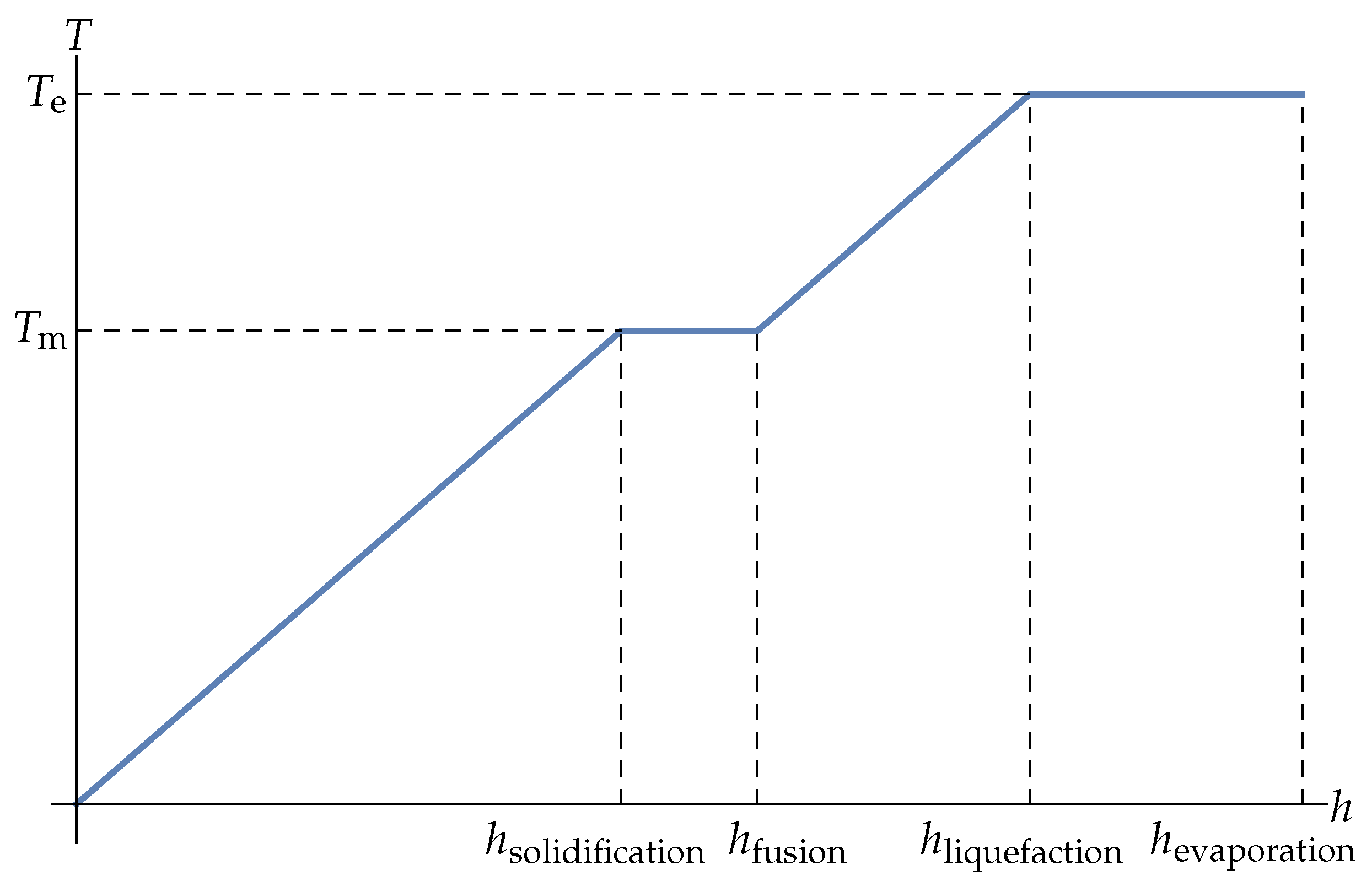
4.3.1. The Enthalpy Method

The challenge associated with the fast treatment of the phase transitions is faced via the use of the so-called enthalpy method. In order to demonstrate the advantages of the enthalpy method, we briefly review the physics of the heat equation.

The heat diffusion equation emerges by the combination of two physical phenomena in one equation. The first phenomenon is the formation of heat currents due to the gradient of the temperature. The second is the variation in the temperature field due to the heat transferred by the heat currents.

The heat current in a homogeneous material is proportional to the temperature gradient. The proportionality constant is by definition the so-called thermal conductivity,

$$\overrightarrow{J}=-k\overrightarrow{\nabla }T.$$

(6)

This is the first part of the phenomenon; the temperature field generates heat currents, determined by the temperature gradients. The second part of the physics is that these heat currents alter the local temperature field. The definition of heat current directly implies that the amount of heat deposited into an elementary volume $dV$ in elementary time $dt$ is equal to

$$\begin{array}{c}\hfill dQ=-\overrightarrow{\nabla }·\overrightarrow{J}dVdt=k{\overrightarrow{\nabla }}^{2}TdVdt.\end{array}$$

(7)

Since the process advances at conditions of constant pressure, it follows that the heat influx adds to the enthalpy content of the volume element. By definition, for the (constant-pressure) specific heat $c_p$, which is defined as the rate of change in the per mass enthalpy density with temperature, it follows that

$$dQ=dH=c_{p}dmdT=c_p\rho dVdT.$$

(8)

This closes the circle; the temperature field and the thermal conductivity determine the heat currents, and the latter combined with the specific heat and the density determine the rate of change of the temperature field. Combining Equations (7) and (8) yields

$${\overrightarrow{\nabla }}^{2}T=\frac{c_p\rho }{k}\frac{\partial T}{\partial t}.$$

(9)

The ratio $\frac{k}{c_p\rho }$ is usually called the thermal diffusivity a. Obviously, if the thermal conductivity, the specific heat, or the density are considered to be non-constant functions of the temperature, the heat equation loses its linear structure and no linear differential equation tools can be applied in order to solve it. Even in this case, a non-linear heat diffusion equation can be solved numerically very easily. This is due to the fact that only the first time derivative of the temperature appears, and, thus, a time stepping, fast-running algorithm can easily be employed. It follows that it is very simple to take into account the dependence of the physical properties on the temperature; it is only necessary to take these dependencies into account at each time step.

However, this cannot be the case in the presence of a phase transition. During a phase transition, the material absorbs heat without changing temperature. When the absorbed heat reaches a certain level, the so-called latent heat, the phase transition is completed, and the temperature starts varying again. Actually, the specific heat at the temperature of a phase transition diverges. Except for the specific heat, other material properties, such as the density or the thermal conductivity, may present significant discontinuities.

A formal analytic calculation of the temperature field in a material undergoing a phase transition requires the study of the heat diffusion equation in separate regions, one for each phase, and a dynamical boundary condition between these regions, which is called the Stefan condition. Let us consider the enlightening example of the melting of a one-dimensional material extending along the z-axis. The formal treatment of this example requires the specification of a boundary between the solid and liquid phases of the material $Z_f\left(t\right)$. Assuming that the solid region is the region $z>Z_f$, one has to solve the equations

$$\frac{{\partial }^2{T}_s}{d{z}^2}=\frac{1}{a_s}\frac{\partial T_s}{\partial t},\frac{{\partial }^2{T}_l}{d{z}^2}=\frac{1}{a_l}\frac{\partial T_l}{\partial t}$$

(10)

in the solid region and liquid regions, respectively, as well as the dynamical Stefan boundary condition

$$-k_l\frac{d{T}_l}{dz}+k_s\frac{d{T}_s}{dz}=L_f\rho \frac{d{Z}_f}{dt},$$

(11)

where $L_f$ is the latent heat of fusion.

This approach is difficult to be realized in the form of a time-stepping fast running algorithm in more than one dimensions. Indeed, it has been successfully used for the modelling of a one-dimensional laser process, e.g., laser drilling [44]. Although the equations still contain only first time derivatives, the regions in which they apply are time-dependent.

It is easier to bypass this problem by introducing a secondary field, that of enthalpy density. Then, instead of solving the heat equation and the Stefan conditions separately, one returns to the fundamental principles that lead to those sets of equations, i.e., the heat currents lead to variations in the enthalpy density field and then, this variation results in a variation in the temperature. The necessary ingredient is the knowledge of an equation of state, namely the relation between enthalpy density and temperature. This relation can be found explicitly from the specific heat and the latent heats and can easily accommodate the dependence of the specific heat on the temperature, even beyond the phase transitions. We will return to this equation of state later in this section.

Let h be the specific enthalpy, i.e., the enthalpy per mass. Having introduced the auxiliary field of the enthalpy density per volume, i.e., $\rho h$, and following the logical steps analysed above, the heat-conduction problem can be formulated as the system of equations

$$\begin{array}{cc}\hfill \frac{\partial \left(\rho h\right)}{\partial t}& =k{\overrightarrow{\nabla }}^{2}T,\hfill \end{array}$$

(12)

$$\begin{array}{cc}\hfill T& =T\left(\rho h\right).\hfill \end{array}$$

(13)

Equation (12) is equivalent to (7), whereas Equation (13) is equivalent to (8). The difference from the basic approach of the heat equation is that (12) and (13) are not combined to form a single equation for the temperature field, in the same logic in which (7) and (8) are combined to form the heat equation.

Equivalently, instead of the enthalpy density, the specific enthalpy density h can be used as the auxiliary field. In this case, the problem is expressed as

$$\begin{array}{cc}\hfill \frac{\partial \left(\rho h\right)}{\partial t}& =k{\overrightarrow{\nabla }}^{2}T,\hfill \end{array}$$

(14)

$$\begin{array}{cc}\hfill T& =T\left(h\right).\hfill \end{array}$$

(15)

Whether the former (enthalpy density) or latter (specific enthalpy) approach is advantageous depends on whether the elements of the simulation lattice are defined to have constant volume or constant mass. This will be answered in the discussion about the multi-scale simulation later on.

At a technical level, the separation of the problem into these two steps splits the original non-linear differential problem in an elegant way. The first step, the one described by Equations (12) or (14), is differential but also linear. The second step, the one described by Equations (13) or (15), is non-linear; however, it is not differential but is algebraic. This greatly simplifies the problem solution. It further allows the direct definition of derivatives as differences and, thus, the formulation of the numerical problem as a finite differences problem, which is a faster and simpler approach than the more flexible but slower widely applied technique of finite elements.

A significant note that has to be made is the fact that a finite differences approach to the solution to the above system of equations sets limits to the time step of the time lattice relative to the lattice constant of the spatial lattice. In order for the numerical algorithm to converge to the solution to the continuous system of equations, it should obey

$$\delta t<\frac{\delta x^2}{2a},\delta t<\frac{\delta y^2}{2a},\delta t<\frac{\delta z^2}{2a},$$

(16)

where a is the thermal diffusivity. Notice that since the thermophysical properties of the material are considered as temperature-dependent; the above criteria should hold at all temperatures. These criteria imply that the finer detail that the spatial lattice must capture, the more time-consuming the algorithm will be, not only because more spatial data have to be manipulated but also because more time steps have to be calculated.

A further important advantage of this approach is that it leads directly to a time-stepping algorithm, an algorithm that can scan the time instant progressively and provide the solution without the need for memory of previous time instants. This is due to the fact that all the fields governing the problem at the time instant $t+dt$ are directly determined by the values of these fields at the time instant t. This fact significantly reduces the resources that are required by the simulation. The enthalpy method has been used for the modelling of laser processes in the past, e.g., laser welding [45].

The enthalpy method directly faces the first main challenge listed in Section 3.3. The fact that it leads to a simple time-stepping finite differences algorithm also leads to the fifth main challenge.

4.3.2. The Division of Modelling to Three Scales

We are mainly left with the third and fourth challenges, as listed in Section 3.3. We would like to confront them without negatively affecting the fifth challenge, namely the creation of a fast-running algorithm. The difficulties related to the third main challenge require the simulation of the process at the micro-scale, i.e., the scale defined by the powder particle dimensions. The adoption of this scale at the simulation of the single track simulation, or at the workpiece level, demands the manipulation of a huge number of data in an obvious manner. It follows that the successful simulation of PBF-LB/M requires the treatment of the process at multiple scales. The output of each level serves as an input for the next one.

At the micro-scale, only a small portion of the raw powder material is considered, and it is simulated as a distribution of solid and empty (and as time evolves and energy flows into the system, liquid also) phases in space, consistent with the distribution of particle dimensions provided by the powder supplier. The main purpose of this simulation is the determination of the mean physical properties of the powder, which serve as an input for the macroscopical-scale simulation after experimental verification.

Then, the meso- and macroscopical simulation is performed. In this stage, a new phase of the material is introduced. The workpiece is simulated as a distribution of powder, solid, and empty (and as time evolves liquid) phases determined by the workpiece geometry. The properties of the powder phase of the material have been determined by the micro-scale simulation.

A great advantage of the enthalpy method is that it can be directly used for the process simulation at all scales, with only minor adaptations, such as the introduction of the extra phase for meso- and macro-scale simulation. Therefore, it can provide a single, unique tool for the complete simulation of the process.

The straightforward treatment of heat diffusion is facilitated by the discretization of the build volume via the introduction of a lattice that is canonical in space. This is the simplest approach due to the fact that the heat currents are determined by the temperature gradient, i.e., the spatial distribution of temperature. However, in AM processes, this straightforward approach presents an important complication. Even if variation in the material density due to thermal expansion or the fusion and solidification phase transitions can be neglected, it certainly cannot be neglected for phase transitions between the powder and liquid phases. This is due to the fact that the powder mass density can be a significant percentage (up to 70%) lower than that of the raw material [46]. This implies that the meso- and macroscopical-scale simulations cannot be based on a static, non-dynamical discretization. On the contrary, each element of the grid must refer to the same amount of mass, and its dimensions must evolve dynamically, depending on the phase of the element (and in general on the temperature). It is considered that a given element of the grid always has the same neighbours; this is a reasonable simplifying assumption due to the local nature of the process. This implies that the enthalpy method should be applied with the definition of the specific enthalpy and not the enthalpy density as the auxiliary field.

Finally, a problem that is difficult to resolve originates from the fact that the meso-scale, which is determined by the laser spot size, and the macro-scale, which is determined by the overall size of the component, may differ by certain orders of magnitude. The laser spot size sets the upper limit for the grid element size. A straightforward discretization at this scale would require an enormous number of data to be held for the whole workpiece.

This can be resolved in a twofold way. As far as the local quality characteristics (porosity, cracking) of the final workpiece are concerned, it suffices to use the intermediate mesoscopic scale. These characteristics are dependent on the temperature gradients at the time of solidification and the material flow, which are determined by the local characteristics of the workpiece, rather than the global ones. Therefore, a mesoscopic scale is large enough to capture the local geometry suffices for this purpose.

The purpose of the analysis of the whole workpiece at the macro-scale is the determination of global properties, such as residual stresses, distortions, and energy efficiency, as well enabling a digital process twin. This analysis requires the introduction of an inhomogeneous grid, which is denser in the regions closer to the laser trajectory. This approach can exponentially reduce the number of data required due to the fact that the nature of the heat equation typically produces exponentially suppressed heat currents as one moves away from the heat sources.

Figure 3 depicts the overview of the global modelling approach.

4.3.3. The Equation of State

As we discussed in Section 4.3.2, the lattice elements should refer to the same amount of mass instead of the same amount of volume, so that expansions and contractions due to temperature changes or phase transitions are easier to incorporate. It follows that the enthalpy method should be applied on the basis of Equations (14) and (15), instead of the Equations (12) and (13). Therefore, the relation between the specific enthalpy and temperature should be found. This approach is also advantageous, since this relation is identical for the solid and powder phases of the material.

As an indicative example, in the simple case, we consider only the solid phase (not the powder phase), liquid phase, and gaseous phase of a metal, and further assume that the specific heat and density are constants at each phase; this equation of state emerges directly from the definition of the specific heat as the derivative

$$c_p={\left.\frac{\partial h}{\partial T}\right|}_P$$

(17)

as well as the definition of the latent heats. This relation reads

$$h=\left\{\begin{array}{cc}{c}_{p\mathrm{s}}T,\hfill & T<T_{\mathrm{m}},\hfill \\ c_{p\mathrm{s}}{T}_{\mathrm{m}}+c_{p\mathrm{l}}\left(T-T_{\mathrm{m}}\right),\hfill & T_{\mathrm{m}}<T<T_{\mathrm{e}}.\hfill \end{array}\right.$$

(18)

The indices s and l refer to the solid and liquid phases of the material, respectively. We are mainly interested in the inverse function of the above, since this provides the temperature as a function of the enthalpy density, which is required for the second step of the enthalpy method, i.e., Equation (15). In this simple case, this looks like

$$T=\left\{\begin{array}{cc}\frac{h}{c_{p\mathrm{s}}},\hfill & h<h_{\mathrm{solidification}},\hfill \\ T_{\mathrm{m}},\hfill & h_{\mathrm{solidification}}<h<h_{\mathrm{fusion}},\hfill \\ T_{\mathrm{m}}+\frac{h-h_{\mathrm{fusion}}}{c_{p\mathrm{l}}},\hfill & h_{\mathrm{fusion}}<H<H_{\mathrm{liquefaction}},\hfill \\ T_{\mathrm{e}},\hfill & h_{\mathrm{liquefaction}}<h<h_{\mathrm{evaporation}},\hfill \end{array}\right.$$

(19)

where

$$\begin{array}{cc}\hfill h_{\mathrm{solidification}}& =c_{p\mathrm{s}}{T}_{\mathrm{m}},\hfill \end{array}$$

(20)

$$\begin{array}{cc}\hfill h_{\mathrm{fusion}}& =h_{\mathrm{solidification}}+L_{\mathrm{f}},\hfill \end{array}$$

(21)

$$\begin{array}{cc}\hfill h_{\mathrm{liquefaction}}& =h_{\mathrm{fusion}}+c_{p\mathrm{l}}\left(T_{\mathrm{e}}-T_{\mathrm{m}}\right),\hfill \end{array}$$

(22)

$$\begin{array}{cc}\hfill h_{\mathrm{evaporation}}& =h_{\mathrm{liquefaction}}+L_{\mathrm{e}}.\hfill \end{array}$$

(23)

The symbols $T_{\mathrm{m}}$ and $T_{\mathrm{e}}$ stand for the melting and evaporation temperature, respectively, whereas the symbols $L_{\mathrm{f}}$ and $L_{\mathrm{e}}$ stand for the specific latent heats of fusion and evaporation, respectively. In this approximation, where the specific heat is considered constant, the relation between the specific heat and temperature look like Figure 4.

In the more general case, where the material parameters are given as a function of the temperature, the above functions must be defined more carefully. More specifically, we have to define the functions

$$\begin{array}{cc}\hfill h_{\mathrm{s}}\left(T\right)& ={\int }_0^T{c}_{p\mathrm{s}}\left(T\right),\hfill \end{array}$$

(24)

$$\begin{array}{cc}\hfill h_{\mathrm{l}}\left(T\right)& =h_s\left(T_{\mathrm{m}}\right)+L_f+{\int }_{T_{\mathrm{m}}}^T{c}_{p\mathrm{l}}\left(T\right),\hfill \end{array}$$

(25)

then,

$$T=\left\{\begin{array}{cc}{h}_{\mathrm{s}}^{-1}\left(h\right),\hfill & h<h_{\mathrm{solidification}},\hfill \\ T_{\mathrm{m}},\hfill & h_{\mathrm{solidification}}<h<h_{\mathrm{fusion}},\hfill \\ h_{\mathrm{l}}^{-1}\left(h\right),\hfill & h_{\mathrm{fusion}}<h<h_{\mathrm{liquefaction}},\hfill \\ T_{\mathrm{e}},\hfill & h_{\mathrm{liquefaction}}<h<h_{\mathrm{evaporation}},\hfill \end{array}\right.$$

(26)

where

$$\begin{array}{cc}\hfill h_{\mathrm{solidification}}& =h_{\mathrm{s}}\left(T_{\mathrm{m}}\right),\hfill \end{array}$$

(27)

$$\begin{array}{cc}\hfill h_{\mathrm{fusion}}& =h_{\mathrm{solidification}}+L_{\mathrm{f}},\hfill \end{array}$$

(28)

$$\begin{array}{cc}\hfill h_{\mathrm{liquefaction}}& =h_{\mathrm{l}}\left(T_{\mathrm{e}}\right),\hfill \end{array}$$

(29)

$$\begin{array}{cc}\hfill h_{\mathrm{evaporation}}& =h_{\mathrm{liquefaction}}+L_{\mathrm{e}}.\hfill \end{array}$$

(30)

In the case of the cubic approximation adopted in this modelling approach, which is described by Equation (3),  Equations (24) and (25) assume the form

$$h_{\mathrm{s}}\left(T\right)=c_{0\mathrm{s}}T+\frac{c_{1\mathrm{s}}}{2}{T}^2+\frac{c_{2\mathrm{s}}}{3}{T}^3+\frac{c_{3\mathrm{s}}}{4}{T}^4$$

(31)

$$\begin{array}{cc}\hfill h_{\mathrm{l}}\left(T\right)& =\left(c_{0\mathrm{s}}-c_{0\mathrm{l}}\right)T_{\mathrm{m}}+\frac{c_{1\mathrm{s}}-c_{1\mathrm{l}}}{2}{T}_{\mathrm{m}}^2+\frac{c_{2\mathrm{s}}-c_{2\mathrm{l}}}{3}{T}_{\mathrm{m}}^3+\frac{c_{3\mathrm{s}}-c_{3\mathrm{l}}}{4}{T}_{\mathrm{m}}^4\hfill \\ & +L_{\mathrm{f}}+c_{0\mathrm{l}}T+\frac{c_{1\mathrm{l}}}{2}{T}^2+\frac{c_{2\mathrm{l}}}{3}{T}^3+\frac{c_{3\mathrm{l}}}{4}{T}^4,\hfill \end{array}$$

(32)

Notice that the information concerning the phase of a volume element can be directly read from the enthalpy density. This is determined by comparing the enthalpy density to the parameters $h_{\mathrm{solidification}}$, $h_{\mathrm{fusion}}$, $h_{\mathrm{liquefaction}}$ and $h_{\mathrm{evaporation}}$.

5. Implementation

The flowchart of the algorithm that implements the physical model is depicted in Figure 5.

Each particular section of the algorithm is discussed below.

5.1. Input Information and Data Structure

5.1.1. Simulation Lattice

We define a Cartesian lattice for all three spatial dimensions, as well as an equidistant lattice for the time instants. Therefore, we need to specify the following

• The maximum x-length XM
• the number of elements in the x-dimension Nx
• The maximum y-length YM
• the number of elements in the x-dimension Ny
• The maximum z-length ZM
• the number of elements in the x-dimension Nz
• The maximum time TM
• the number of time steps Nt

It is assumed that the lattice initially comprises elements with dimensions $\mathtt{d}\mathtt{x}\times \mathtt{d}\mathtt{y}\times \mathtt{d}\mathtt{z}=\mathtt{X}\mathtt{M}/\mathtt{N}\mathtt{x}\times \mathtt{Y}\mathtt{M}/\mathtt{N}\mathtt{y}\times \mathtt{Z}\mathtt{M}/\mathtt{N}\mathtt{z}$. A step of the time-stepping algorithm has the duration $\mathtt{d}\mathtt{t}=\mathtt{T}\mathtt{M}/\mathtt{N}\mathtt{t}$.

5.1.2. Data Structure

We define the following arrays

• A double precision three-dimensional array for the temperature, T(i,j,k), which takes values at each lattice cell;
• A double precision three-dimensional array for the enthalpy density, H(i,j,k), which takes values at each lattice cell;
• A boolean three-dimensional array, IsSolid(i,j,k), providing the information of whether a specific cell is in the solid state, which takes values at each lattice cell;
• A boolean three-dimensional array, IsPowder(i,j,k), providing the information of whether a specific cell is in the powder state, which takes values at each lattice cell;
• A boolean three-dimensional array, IsLiquid(i,j,k), providing the information of whether a specific cell is in the liquid state, which takes values at each lattice cell;
• A boolean three-dimensional array, IsEmpty(i,j,k), providing the information of whether a specific cell is in the gaseous state or it is empty, which takes values at each lattice cell;
• Three double precision three dimensional arrays dx(i,j,k), dy(i,j,k) and dz(i,j,k) for the dimensions of the lattice cells, in order to take into account the phenomenon of expansion and contraction;
• A double precision three-dimensional array for the mass of each cell, m(i,j,k);
• An integer two-dimensional array, Top(i,j), which takes values at each x and y position of the lattice, which indicates the first cell at the corresponding vertical column of the lattice which is not empty, and, thus, the cell which is directly hit by the laser beam.

5.1.3. Material Properties

For each of the states of the material, it is required to know

• The density $\rho$;
• The specific heat $c_p$;
• The thermal conductivity k.

These quantities should be given as functions of the temperature, $\rho \left(T\right)$, $c_p\left(T\right)$, and $k\left(T\right)$. In this modelling approach, these quantities are determined by a set of four parameters for each phase; therefore, there are a total of twelve parameters for each quantity, which determine a cubic-order polynomial, which describes the variation in the quantity with temperature, in the form of Equations (1)–(3).

It is further required to provide

• The melting temperature $T_{\mathrm{m}}$;
• The latent heat of fusion $L_{\mathrm{f}}$;
• The evaporation temperature $T_{\mathrm{e}}$;
• The latent heat of evaporation $L_{\mathrm{e}}$.

The above forty quantities, which determine a material for the purposes of the simulation, should be used to define the function TofH, which relates the temperature to enthalpy density. This is achieved through the Formula (26).

The function $T\left(h\right)$ is expressed in terms of the parameters $h_{\mathrm{solidification}}$, $h_{\mathrm{fusion}}$, $h_{\mathrm{liquefaction}}$, and $h_{\mathrm{evaporation}}$, which are calculated via the Equations (27)–(30). These four parameters should be calculated and explicitly stored in constant variables HSolid, HFusion, Hliq, and HEvap. They are significant input of the algorithm as they are necessary to find the phase of a lattice cell as function of its enthalpy.

5.1.4. Laser Beam Properties

The following input is required for the laser source

• The laser beam power P;
• The radius of the laser spot $r_0$;
• The orbit of the laser beam spot, i.e., the two functions of time $x_l\left(t\right)$ and $y_l\left(t\right)$.

The above data should be used to define the functions Intensity(t,x,y) and Power(t,i,j) through the Equations (4) and (5), respectively.

5.1.5. Material–Laser Interaction

A very important property that has to be taken into account is the material reflectivity. This is a very important factor since for most metals this ranges from 70% to 90%. For the micro configurations, but also in cases where a significant keyhole is formed, it is important to take into account the dependence of reflectivity on the angle of incidence ${\theta }_i$.

• Reflectivity as function of the angle of incidence $R\left({\theta }_i\right)$

5.1.6. The Initial State of the Workpiece

Two kinds of data should be provided as description of the initial state of the system.

• The initial temperature and the initial specific enthalpy field;
• The initial distribution of phases in the system.

This may look like a lot of detailed data for input; however, as far as the first kind of data area considered,

• The initial temperature for the first layer is simply a homogeneous temperature field equal to the environment temperature $T_0$;
• The initial temperature for the next layers can be simply the output of the previous layer and a cooling/powder reloading phase.

Therefore, this kind of data can be reduced to a single parameter, the environment temperature $T_0$. This parameter can be controlled through a pre-heating phase. It is a process parameter that significantly influences energy efficiency and quality characteristics of the final workpiece.

As far as the second kind of data are considered,

• In the case of meso and macro configurations, for the first layer, the initial configuration is rather trivial, as only a single, constant-depth layer of powder exists. For the next layers, the initial configuration is simply the outcome of the previous layer and a cooling/powder reloading phase.
• In the case of micro configurations, this kind of data can be quite complicated, since they should simulate the shape, distribution, and size of the powder particles. In these cases, though the initial configuration contains only two phases, the solid and the empty, unlike the macro configurations, where in general three phases may be present, the phases can be solid, powder, and empty.

The second kind of data should be used to determine the initial value of the array Top(i,j), which specifies the location of the top surface. This is just the index of the minimum z element, for every i and j that is not empty.

5.2. Boundary Conditions

In order to completely define the numerical problem, we need to also define the boundary conditions. There are two extremal cases that can be considered.

• Dirichlet conditions: The whole lattice box is considered to be in contact with an environment with a large heat capacity, which completely sets the temperature of the boundary.
• Neumann conditions: the whole lattice box is considered to be thermally isolated from its environment.

Intermediate boundary conditions, which are linear combinations of the above extremal cases, can also be considered. In order to determine this kind of intermediate conditions, a double precision variable Dirichlet is defined, which takes values between 0 and 1. The value 0 corresponds to Neumann conditions, whereas the value 1 corresponds to Dirichlet conditions.

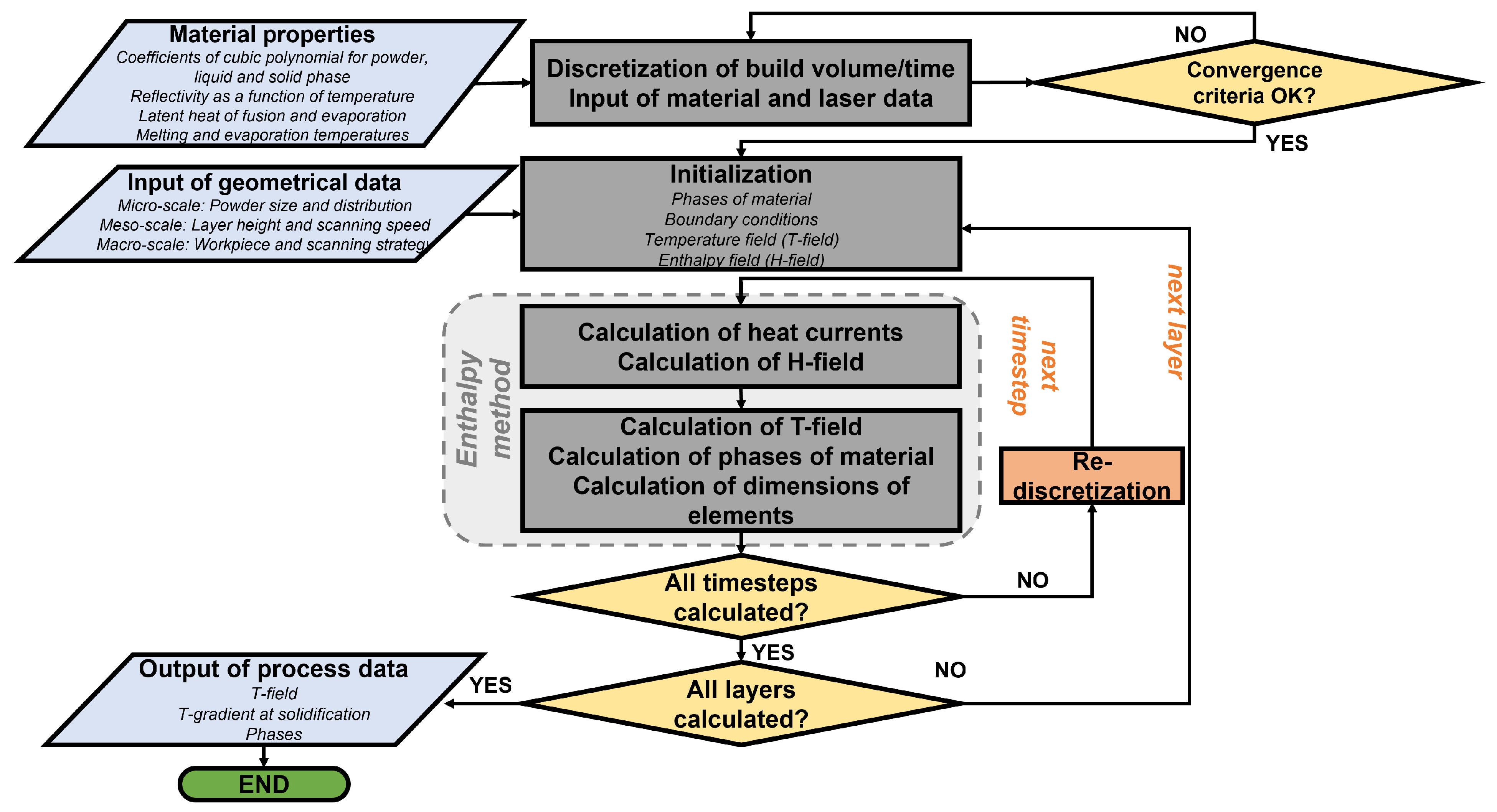
5.3. The Time-Stepping Algorithm

The first step in the time-stepping algorithm is the calculation of the heat currents at each element. Four integer variables are introduced, t for the time latticing, i for the x latticing, j for the y latticing, and k for the z latticing

• Initiate a loop for time starting from t = 1;
• Initiate a loop for x from i = 1, initiate a loop for y from j = 1 and finally initiate a loop for z from k = Top(i,j), i.e., initiate each vertical column from its top element to its depths;
• Use Formula (6) to calculate the heat current from the left, right, front, back, top and bottom. For example, the incoming heat current from the left is

  $$\mathtt{L}\mathtt{c}\mathtt{u}\mathtt{r}\mathtt{r}\mathtt{e}\mathtt{n}\mathtt{t}=\mathtt{k}\ast \left(\mathtt{T}\right(\mathtt{i}-\mathtt{1},\mathtt{j},\mathtt{k})-\mathtt{T}(\mathtt{i},\mathtt{j},\mathtt{k}\left)\right)/\mathtt{d}\mathtt{x}$$

  (33)

  and from the right is

  $$\mathtt{R}\mathtt{c}\mathtt{u}\mathtt{r}\mathtt{r}\mathtt{e}\mathtt{n}\mathtt{t}=\mathtt{k}\ast \left(\mathtt{T}\right(\mathtt{i}+\mathtt{1},\mathtt{j},\mathtt{k})-\mathtt{T}(\mathtt{i},\mathtt{j},\mathtt{k}\left)\right)/\mathtt{d}\mathtt{x}$$

  (34)
  The conductivity in the above example should be taken as the conductivity of the neighbouring lattice element, that is to say the conductivity referring to the phase of the neighbouring element at the temperature of this neighbouring element. For example, in the above formula for the left current, k should be considered the conductivity of the element (i − 1,j,k). This ensures that to heat current is going to be calculated when the neighbouring element is empty.
  Notice also that since the lattice elements may have different dimensions, the variable dx in the above formulae should be calculated as the average of the parameter dx for the two involved lattice cells.
  • In an obvious manner the formula for the left current is problematic when i = 1. This specific left current is calculated via the boundary conditions. If Neumann conditions are applied, then this left current vanishes. If Dirichlet boundary conditions are applied, then it is considered that the element to the left lies at the environment temperature T0 and therefore

    $$\mathtt{L}\mathtt{c}\mathtt{u}\mathtt{r}\mathtt{r}\mathtt{e}\mathtt{n}\mathtt{t}=\mathtt{k}\ast (\mathtt{T}\mathtt{0}-\mathtt{T}(\mathtt{1},\mathtt{j},\mathtt{k}\left)\right)/\mathtt{d}\mathtt{x}$$

    (35)
    In the more generic case of intermediate boundary conditions it holds that

    $$\mathtt{L}\mathtt{c}\mathtt{u}\mathtt{r}\mathtt{r}\mathtt{e}\mathtt{n}\mathtt{t}=\mathtt{D}\mathtt{i}\mathtt{r}\mathtt{i}\mathtt{c}\mathtt{h}\mathtt{l}\mathtt{e}\mathtt{t}\ast \mathtt{k}\ast (\mathtt{T}\mathtt{0}-\mathtt{T}(\mathtt{1},\mathtt{j},\mathtt{k}\left)\right)/\mathtt{d}\mathtt{x}$$

    (36)
    Similar care should be taken for the right current when i = XM, the front current when j = 1, the back current when j = YM and the bottom current when k = ZM.
  • from the currents calculate the influx of energy from each direction. For example, the influx from the left will be

    $$\mathtt{L}\mathtt{f}\mathtt{l}\mathtt{u}\mathtt{x}=\mathtt{L}\mathtt{c}\mathtt{u}\mathtt{r}\mathtt{r}\mathtt{e}\mathtt{n}\mathtt{t}\ast \mathtt{d}\mathtt{y}\ast \mathtt{d}\mathtt{z}\ast \mathtt{d}\mathtt{t}$$

    (37)
    Notice that since the lattice elements may have different dimensions, the variables dy and dz in the above formulae should be calculated as the average of the corresponding parameters for the two involved lattice cells.
  • If k = Top(i,j) calculate the top influx from the laser power function reduced by the reflectivity factor
• Recalculate the enthalpy ingredient of the element (i,j,k), using the formula

  $$\mathtt{H}(\mathtt{i},\mathtt{j},\mathtt{k})=\mathtt{H}(\mathtt{i},\mathtt{j},\mathtt{k})+(\mathtt{L}\mathtt{c}\mathtt{u}\mathtt{r}\mathtt{r}\mathtt{e}\mathtt{n}\mathtt{t}+\mathtt{R}\mathtt{c}\mathtt{u}\mathtt{r}\mathtt{r}\mathtt{e}\mathtt{n}\mathtt{t}+...)/\mathtt{m}(\mathtt{i},\mathtt{j},\mathtt{k})$$

  (38)
• Advance z loop, advance y loop, advance x loop.
• Initiate a loop for x from i = 1, initiate a loop for y from j = 1 and finally initiate a loop for z from k = Top(i,j).
• If the enthalpy density is larger than the value HEvap, we should give to IsEmpty(i,j,k) the value True, and we should give to the rest of the Boolean variables at (i,j,k) the value False and add one to the Top(i,j).
• Else If the enthalpy density is larger than the value HFusion and IsPowder(i,j,k) is True, then, give the value False to IsPowder(i,j,k), the value True to IsLiquid(i,j,k).
• Else If the enthalpy density is larger than the value HFusion and IsSolid(i,j,k) is True, then, give the value False to IsSolid(i,j,k), the value True to IsLiquid(i,j,k).
• Else If the enthalpy density is smaller than the value HSolid and IsLiquid(i,j,k) is True, then, give the value False to IsLiquid(i,j,k), the value True to IsSolid(i,j,k).
• Recalculate the temperature of the element from its enthalpy density using the function TofH
• Recalculate the dimensions of the element using the function of the mass density.
• Advance z loop, advance y loop, advance x loop.
• Advance the time loop.

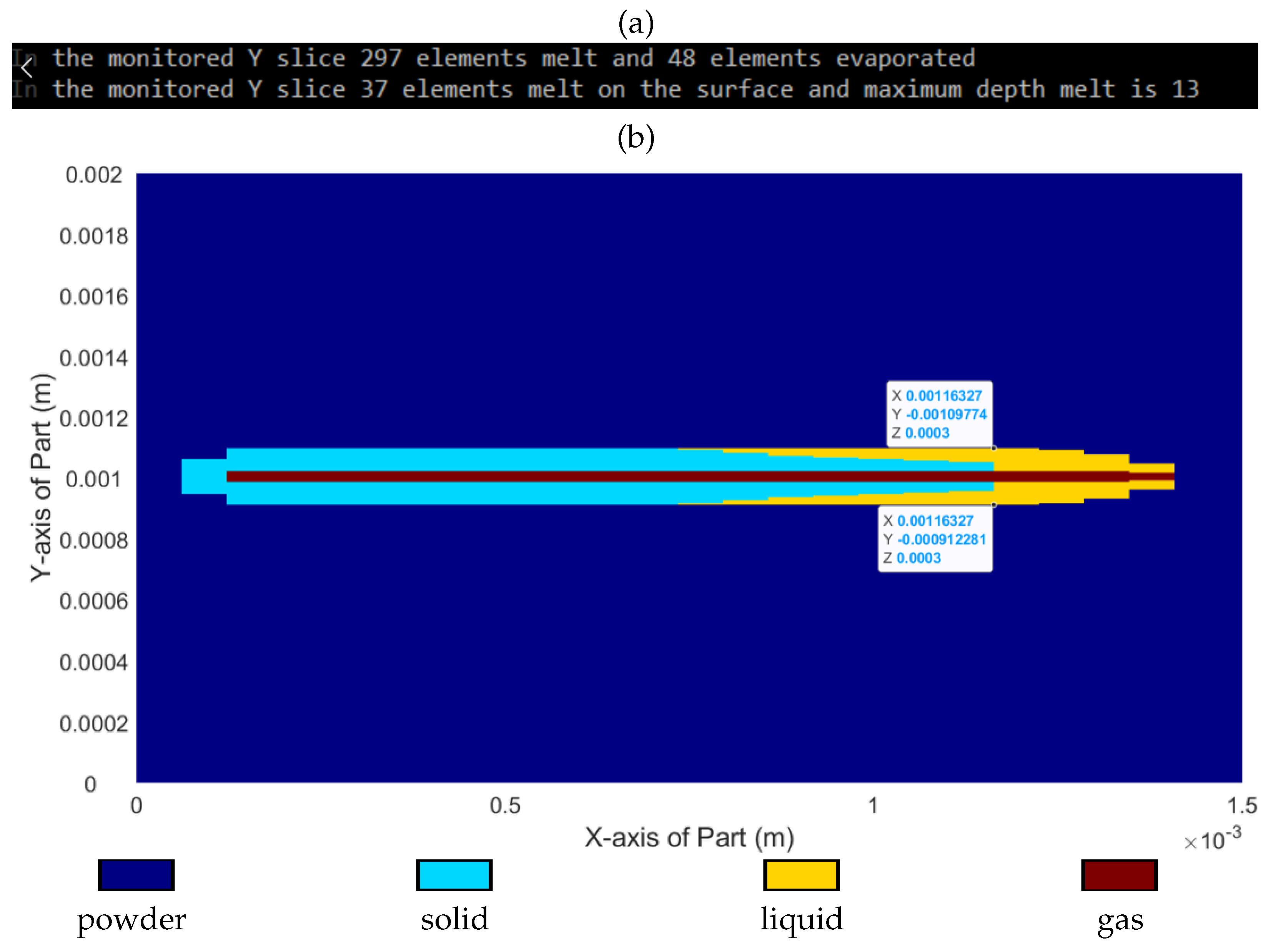
6. Model Validation and Results

The validation of the model requires several steps aiming to point out accuracy and adaptability in various conditions, where the inputs related to material properties, laser beam properties and combination of process parameters vary. Before comparing the numerical outputs of the model related to the melt pool geometrical features to experimental results in the literature, extensive preparatory work has been carried out. The mesh density and the dimensions of each element have been decided after sensitivity analysis in all three spatial dimensions until convergence, also considering the computational time/power as criteria for the decision making. Additionally, the effect of boundary conditions (the value of the Dirichlet parameter) and the overall dimensions of the bounding box on the model outputs have been investigated. The overall box dimensions were selected so that the result is not significantly sensitive to the form of the boundary conditions. Finally, the trend of outputs has been studied by investigating if they satisfy physics-based and process-based rules when providing different combination of process inputs.

Overall, the model is able to characterize the stability of the process conduction mode–keyhole mode) by comparing the dimensions of melt pool width and depth [26], as well as the volume of the material that is in gaseous phase compared to the volume of material that is molten. Moreover, by visually inspecting the temperature and phase plots, the information about the governing mode and the process stability can be extracted. The aforementioned relation between the process parameters and the process stability will be discussed in a follow-up of this work, while this work emphasizes the demonstration of the predictive capability of the model in two different materials with different combinations of process inputs, as well as on the overall structure of the model as it is presented in Section 3, Section 4 and Section 5.

The model has significant predictive capability as it regards melt pool width when the process is stable (conduction mode). The accuracy of the model has been validated by examining two (stable) processes from the literature with experimental data, which are related to Ti6Al4v [47] and SS316L [48]. The simulation omits material movements due to surface tensions. Therefore, it is more suitable to compare the model predictions with results from process monitoring devices that capture the melt pool geometrical features in real time. When the results are compared with outputs from microscopes and some significant deviations are detected due to the effect of surface tension and thermal shrinkage on the overall dimensions [47,48], the latter can be easily incorporated adding a cooling phase in the simulation.

The studied cases are both single tracks, where the substrate has been covered with one layer of powder to simulate processing conditions. The Ti6Al4v case has been performed in a PBF-LB/M machine of KU Leuven. The powder particle size ranged from 15 to 45 $\mathsf{\mu }$m. The Ti6Al4v substrate plate dimensions were $10\times 10\times 5$ mm, and the melt pool characteristics were acquired with a coaxial monitoring set up. The accuracy of the monitoring set up is determined from the pixel size, which was equal to 14 $\mathsf{\mu }$m [47]. On the other hand, the SS316L case has been performed at a custom-made PBF-LB/M machine with an integrated coaxial melt pool monitoring set up [48]. The powder particle size ranged from 10 to 45 $\mathsf{\mu }$m, and the SS316L substrate plate was selected to be equal to $25\times 15\times 1.5$ mm. The accuracy of the monitoring system was equal to $11.8$ $\mathsf{\mu }$m. For both cases, the melt pool features were extracted with image processing algorithms that were implemented in a MATLAB environment.

The model considers temperature-dependent thermophysical properties for the powder, liquid, and solid phases for both materials. The first part of the simulation was the micro-scale modelling of the powder, in order to acquire the powder’s thermal conductivity. The latter depends on the solid thermal conductivity but also on the powder particles geometry. For the clarity of presentation, the powder particles were considered to form a cubic lattice with a period equal to the mean powder particle diameter, namely 30 $\mathsf{\mu }$m for the Ti6Al4v case and 27.5 $\mathsf{\mu }$m for the SS316L case. The dimensions of the contact interface between the powder particles were considered to be equal to $1/10$ of the dimension of the powder particles [40]; the area of the interface was considered equal to $9 {\left(\mathsf{\mu }\mathrm{m}\right)}^2$ in the Ti6Al4v case and $7.5 {\left(\mathsf{\mu }\mathrm{m}\right)}^2$ in the SS316L case.

The micro-scale model simulated the powder for a given amount of time and a considered homogeneous influx of energy coming from the top horizontal surface of the simulated sample. The temperature field is shown in Figure 6.

Then, the same volume was considered to be occupied by an effective homogeneous material, with the same specific heat as the solid phase, the same mass density as the mean mass density of the lattice simulated above, and an effective thermal conductivity, which is a fraction of the thermal conductivity of the solid phase of Ti6Al4v or SS316L, respectively. This sample was simulated for the same amount of time and the same influx of energy as the lattice, for various values of the effective thermal conductivity, in a search for the effective thermal conductivity, which reproduces an equivalent mean thermal behavior as the powder particle lattice. The mean temperature at each horizontal plane as a function of the depth is compared for each effective thermal conductivity with that in the case of the lattice in Figure 7.

The mean temperature as a function of depth was fit by a third-order polynomial in each case. The parameters of the polynomial fit for the effective homogeneous material present maximum proximity to those of the lattice for

$$k_{\mathrm{eff}}=\left(0.053\pm 0.005\right)k_{\mathrm{s}}.$$

(39)

This value is very close to the value $k_{\mathrm{eff}}=0.05k_{\mathrm{s}}$ found in the literature [37], which is the value of the mean effective thermal conductivity of the powder that we use in the meso-scale simulation below.

The meso-scale simulation requires temperature-dependent thermophysical properties for the powder, liquid, and solid phases for both materials. The coefficients for the cubic polynomial in these three phases have been acquired after experimental work, and they have been identified in the literature [43,49,50,51]. In Section 3.2.2, the effect of powder particle geometry on the reflectivity of powder bed has been discussed; thus, for both cases, the reflectivity coefficient has been considered a function of the phase (powder, solid, and liquid) and the relevant values have been retrieved from the literature [39,52]. The model inputs for both cases are included in

Table 1. Model inputs for the validation with the Ti6Al4v [47] case and the SS316L [48] case.

Parameter	Ti6Al4v	SS316L	Units
Power	170	500	$\mathrm{W}$
Speed	1000	600	$\mathrm{mm}/\mathrm{s}$
Laser spot size	37.5	19.5	$\mathsf{\mu }\mathrm{m}$
Layer thickness	30	30	$\mathsf{\mu }\mathrm{m}$
Substrate material	Ti6Al4v	SS316L
Reflectivity of powder	0.3	0.24	-
Reflectivity of solid	0.7	0.58	-
Reflectivity of liquid	0.6	0.38	-
Melting temperature	1660	1400	${}^{\circ }\mathrm{C}$
Evaporation temperature	2860	2800	${}^{\circ }\mathrm{C}$
Latent heat of fusion	286	260	$\mathrm{kJ}/\mathrm{kg}$
Latent heat of evaporation	9830	7450	$\mathrm{kJ}/\mathrm{kg}$

. The polynomials fitting the conductivity, specific heat, and mass density of the materials used in the case studies are shown in

Table 2. Thermophysical properties of Ti6Al4v and SS316L [43,49,50,51].

Parameter	Ti6Al4v
$k_{\mathrm{p}}$	$0.3155\frac{\mathrm{W}}{\mathrm{m}·\mathrm{K}}+\left(1.36\times {10}^{-3}\frac{\mathrm{W}}{\mathrm{m}·{\mathrm{K}}^2}\right)T$
$k_{\mathrm{s}}$	$6.31\frac{\mathrm{W}}{\mathrm{m}·\mathrm{K}}+\left(2.72\times {10}^{-2}\frac{\mathrm{W}}{\mathrm{m}·{\mathrm{K}}^2}\right)T-\left(7\times {10}^{-6}\frac{\mathrm{W}}{\mathrm{m}·{\mathrm{K}}^3}\right)T^2$
$k_{\mathrm{l}}$	$6.6\frac{\mathrm{W}}{\mathrm{m}·\mathrm{K}}+\left(1.214\times {10}^{-2}\frac{\mathrm{W}}{\mathrm{m}·{\mathrm{K}}^2}\right)T$
$c_{p\mathrm{p}}$/$c_{p\mathrm{s}}$	$412\frac{\mathrm{J}}{\mathrm{kg}·\mathrm{K}}+\left(0.2\frac{\mathrm{J}}{\mathrm{kg}·{\mathrm{K}}^2}\right)T-\left(2\times {10}^{-5}\frac{\mathrm{J}}{\mathrm{kg}·{\mathrm{K}}^3}\right)T^2$
$c_{p\mathrm{l}}$	$790\frac{\mathrm{J}}{\mathrm{kg}·\mathrm{K}}$
${\rho }_{\mathrm{p}}$	$4065.355\frac{\mathrm{kg}}{{\mathrm{m}}^3}-\left(0.385\frac{\mathrm{kg}}{{\mathrm{m}}^3·\mathrm{K}}\right)T$
${\rho }_{\mathrm{s}}$	$8099.298\frac{\mathrm{kg}}{{\mathrm{m}}^3}-\left(0.501\frac{\mathrm{kg}}{{\mathrm{m}}^3·\mathrm{K}}\right)T$
${\rho }_{\mathrm{l}}$	$8130.71\frac{\mathrm{kg}}{{\mathrm{m}}^3}-\left(0.77\frac{\mathrm{kg}}{{\mathrm{m}}^3·\mathrm{K}}\right)T$
Parameter	SS316L
$k_{\mathrm{p}}$	$0.079\frac{\mathrm{W}}{\mathrm{m}·\mathrm{K}}+\left(3.276\times {10}^{-4}\frac{\mathrm{W}}{\mathrm{m}·{\mathrm{K}}^2}\right)T$
$k_{\mathrm{s}}$	$4.7\frac{\mathrm{W}}{\mathrm{m}·\mathrm{K}}+\left(3.1\times {10}^{-3}\frac{\mathrm{W}}{\mathrm{m}·{\mathrm{K}}^2}\right)T+\left(1\times {10}^{-5}\frac{\mathrm{W}}{\mathrm{m}·{\mathrm{K}}^3}\right)T^2-\left(3\times {10}^{-9}\frac{\mathrm{W}}{\mathrm{m}·{\mathrm{K}}^4}\right)T^3$
$k_{\mathrm{l}}$	$34\frac{\mathrm{W}}{\mathrm{m}·\mathrm{K}}$
$c_{p\mathrm{p}}$/$c_{p\mathrm{s}}$	$533.07\frac{\mathrm{J}}{\mathrm{kg}·\mathrm{K}}+\left(0.0496\frac{\mathrm{J}}{\mathrm{kg}·{\mathrm{K}}^2}\right)T+\left(4\times {10}^{-5}\frac{\mathrm{J}}{\mathrm{kg}·{\mathrm{K}}^3}\right)T^2+\left(4\times {10}^{-9}\frac{\mathrm{J}}{\mathrm{kg}·{\mathrm{K}}^4}\right)T^3$
$c_{p\mathrm{l}}$	$830\frac{\mathrm{J}}{\mathrm{kg}·\mathrm{K}}$
${\rho }_{\mathrm{p}}$	$2459.3\frac{\mathrm{kg}}{{\mathrm{m}}^3}-\left(0.1255\frac{\mathrm{kg}}{{\mathrm{m}}^3·\mathrm{K}}\right)T+\left(4\times {10}^{-5}\frac{\mathrm{kg}}{{\mathrm{m}}^3·{\mathrm{K}}^2}\right)T^2-\left(1\times {10}^{-8}\frac{\mathrm{kg}}{{\mathrm{m}}^3·{\mathrm{K}}^3}\right)T^3$
${\rho }_{\mathrm{s}}$	$4471.4\frac{\mathrm{kg}}{{\mathrm{m}}^3}-\left(0.2282\frac{\mathrm{kg}}{{\mathrm{m}}^3·\mathrm{K}}\right)T+\left(8\times {10}^{-5}\frac{\mathrm{kg}}{{\mathrm{m}}^3·{\mathrm{K}}^2}\right)T^2-\left(2\times {10}^{-8}\frac{\mathrm{kg}}{{\mathrm{m}}^3·{\mathrm{K}}^3}\right)T^3$
${\rho }_{\mathrm{l}}$	$3920\frac{\mathrm{kg}}{{\mathrm{m}}^3}$

.

The model outputs for both cases compared to the measurements from the process monitoring are presented in

Table 3. Model validation with experimental data from process monitoring with high-speed coaxial cameras in the Ti6Al4v case study [47] and the SS316L case study [48].

Case Study				Melt Pool Width ($\mathsf{\mu }\mathbf{m}$)
Material	Power ($\mathrm{W}$)	Speed ($\mathrm{mm}/\mathrm{s}$)	In Line Monitoring	Model Output
Ti6Al4v	170	1000	$179\pm 13$	$185\pm 5$
SS316L	500	600	$127\pm 44$	$170\pm 3$

. The process monitoring captures only the melt pool width and, thus, only the melt pool width value will be compared. The melt pool depth is usually extracted with empirical rules that relies on the measured melt pool width and the process inputs [53]. Thus, there is no way to compare the model outputs with data from process monitoring but only with data from a microscope. The required correction factor that will match the melt pool depth predictions and the measurements from a microscope will be included in the second part of this work.

The error for the in-line measurements is introduced from the pixel size, while from the model side, the element dimensions determine the accuracy of the result. The melt pool width is extracted by measuring the related dimension from the phase plot or by multiplying the molten elements with the width size of each element. Both methods are depicted in Figure 8. As far as the correspondence of the simulation with the experimental results is concerned, especially regarding the SS316L case, a simulation result may appear that is quite distant from the in-line monitoring measurement. However, in this case, the in-line monitoring measurement has a much larger uncertainty than in the Ti6Al4V case: the melt pool width measurement lies within the range of 83–171 $\mathsf{\mu }\mathrm{m}$. The predicted value from the simulation lies within this range. In the Ti6Al4V case, the measurement uncertainty is much smaller. In this case, the simulated melt pool width is significantly closer to the central measured value from the in-line monitoring.

In Figure 9, the temperature distribution and the phase change along the width direction are provided for each of the studied cases.

Figure 10 depicts the same information but in a vertical plane.

The trend of temperature field across the height as well as the phases across the height are studied and compared to literature sources. The validation considers only the melt pool width since the melt pool depth cannot be measured in line. The main scope of the article is to demonstrate the enthalpy method as an enabler for fast simulation of Powder Bed Fusion, and a very limited validation is provided. A follow-up to this work is planned where an extended validation sequence will also be conducted. Although the accuracy of the melt pool depth is not evaluated in this work, it is important to mention that the model adapts to the distinct characteristics of each case while both profiles are also validated with literature sources [51,54,55,56].

As can be seen in these two cases, the effect of laser spot size on the temperature and phase profile is obvious. Although the width dimensions are similar, the temperature and phase distribution point out that in the case with the smaller laser spot, a larger gas phase is met due to localized effect of laser power and small speed. However, in both cases, the stability of the process has been evaluated bty comparing the melt pool width and depth dimensions. In the case that is related to Ti6Al4v [47], the effect of high speed and lower laser power on the melt pool depth dimensions can be identified, while on the other hand, for the SS316L [48], a significantly larger melt pool depth is predicted due to the higher laser power and reduced speed.

The computational efficiency of the proposed method is proven by the fact that the meso-scale simulation requires approximately 30 min of wall clock time on a typical PC (Intel Core I7-9850H CPU @ 2.60 GHz, 16 GB of RAM) without fine-tuning the mesh size and density. Indicatively, the domain size was $2\mathrm{mm}\times 3\mathrm{mm}\times 3\mathrm{mm}$ with a cell size of $5\mathsf{\mu }\mathrm{m}\times 60\mathsf{\mu }\mathrm{m}\times 4.29\mathsf{\mu }\mathrm{m}$. The transient simulation was running for a simulation time of $0.25\mathrm{ms}$ with a time step of $0.025\mathsf{\mu }\mathrm{s}$. The proposed model provides a significantly lower computational time than traditional methods [57] without compromising the simulation resolution that is often an impact of other proposed methods for computation time reduction in PBF-LB/M modelling [58].

The micro-scale is about one order of magnitude slower due to the need for a much denser lattice, which is able to capture the interfaces between the powder particles. The simulation of the powder lattice requires about 18 h on a desktop configuration used for engineering simulations (Intel Core I7-7820X CPU @ 3.60 GHz, 64 GB of RAM). The micro-scale simulation of the equivalent homogeneous material required 45 min to 6 h depending on the effective thermal conductivity on the same computer. The domain size was $150\mathsf{\mu }\mathrm{m}\times 150\mathsf{\mu }\mathrm{m}\times 90\mathsf{\mu }\mathrm{m}$ with a cell size of $1\mathsf{\mu }\mathrm{m}\times 1\mathsf{\mu }\mathrm{m}\times 1\mathsf{\mu }\mathrm{m}$. The simulation time included 80,000 time steps of the algorithm. It has to be noticed that the micro-scale simulation is a task that must be performed only once per material used, and, thus, these higher time requirements can be more easily tolerated.

7. Conclusions

The modelling approach that relies on the division of the working envelope in three scales and the enthalpy method, as well as the careful treatment of challenges that are met in AM (Section 3.3), led to the development of a fast-running simulation algorithm. The algorithm has significant predictive capability regarding the melt pool width calculation and provision of outputs that can be used for process stability evaluation. This fast-delivered information can be used in an industrial environment to determine the process window of a new machine material by indicating which combination of process inputs could lead to non-stable process. Furthermore, it provides the melt pool dimensions, which are critical for the development of the path-planning strategy where the overlap between consecutive tracks should be determined. As future work, the further study and the extensive validation of the model outputs, as well as the integration of the additional features that are presented in the discussion section and their outputs, will be performed.

8. Discussion

As mentioned in Section 6, the validation process has been divided into several steps so as to extract secure conclusions about the quality of the model predictions. This work summarizes the workflow that has been followed in order to develop a multi-functional model that is able to predict with high accuracy the powder-bed thermophysical properties (micro-scale), the melt pool dimensions during the process, the volume of material in gaseous phase, and the molten material, as well as the temperature field and the spatial distribution of material phases (meso-scale). The validation of these outputs is very important in order to enable the development of additional functionalities that rely on these outputs as well as on complementary features that will be integrated on the existing model and will be presented in future works.

The powder particle-size distribution is used so as to develop a packing model that will simulate a sample of an actual powder bed. A custom packing model, similar to the rain model [59], will be integrated for this purpose. Additionally, a Monte Carlo model [60] will be used to calculate the actual reflectivity and absorptivity of the powder bed as a function of the powder particle size distribution. These modules will be an improvement to the micro-scale model, which will provide more accurate input data to the meso- and macro-scale simulation.

The meso- and macro-scale simulation will be used for the prediction of energy efficiency as a function of process parameters (meso-scale) and path planning strategy (macro-scale). Furthermore, the temperature field is the information needed to calculate the residual stresses. The aforementioned will be tested and validated with experimental works in various non-trivial geometries.

Another significant benefit of this modelling approach is the capability to adopt different beam-shaping techniques, as presented in [61]. In this specific work, only the Gaussian intensity profile has been used. Additionally, with the aid of different beam-shaping techniques, the process performance and efficiency will be studied for a variety of materials and process parameters [62]. This information will identify the significance of the developed virtual test bed that will try to tackle a common issue that is met in AM processes where the material is overheated in the laser spot center due to an excess of energy, which leads to significant material evaporations, and the material at the periphery of the spot does not have the necessary processing temperature [61]. Thus, a lot of energy is lost by heat diffusion in the treated body.

Finally, by taking advantage of the structure of the model, it is easy to substitute the properties of the powder bed into solid material, and other laser-based processes can be simulated, such as laser cutting, laser drilling, and laser welding. The heat affected zone and the developed residual stresses near the welded, drilled, or cut area can be predicted with the same model.

References

1. ISO/ASTM 52911-1; Additive Manufacturing—Design—Part 1: Laser-Based Powder Bed Fusion of Metals. International Organization for Standardization: Geneva, Switzerland, 2019.
2. Stavropoulos, P.; Foteinopoulos, P. Modelling of additive manufacturing processes: A review and classification. Manuf. Rev. 2018, 5, 26. [Google Scholar] [CrossRef] [Green Version]
3. AMPOWER Report 2022. Available online: https://additive-manufacturing-report.com/ (accessed on 2 August 2022).
4. Schmidt, M.; Merklein, M.; Bourell, D.; Dimitrov, D.; Hausotte, T.; Wegener, K.; Overmeyer, L.; Vollertsen, F.; Levy, G.N. Laser based additive manufacturing in industry and academia. CIRP Ann. 2017, 66, 561–583. [Google Scholar] [CrossRef]
5. HUBS. Additive Manufacturing Trend Report 2021. 2021. Available online: https://www.hubs.com/get/trends/ (accessed on 8 April 2022).
6. Stavropoulos, P.; Papacharalampopoulos, A.; Michail, C.K.; Chryssolouris, G. Robust additive manufacturing performance through a control oriented digital twin. Metals 2021, 11, 708. [Google Scholar] [CrossRef]
7. Sanaei, N.; Fatemi, A. Defects in additive manufactured metals and their effect on fatigue performance: A state-of-the-art review. Prog. Mater. Sci. 2021, 117, 100724. [Google Scholar] [CrossRef]
8. Gunasegaram, D.R.; Murphy, A.B.; Barnard, A.; DebRoy, T.; Matthews, M.J.; Ladani, L.; Gu, D. Towards developing multiscale-multiphysics models and their surrogates for digital twins of metal additive manufacturing. Addit. Manuf. 2021, 46, 102089. [Google Scholar] [CrossRef]
9. ElMaraghy, H.; Monostori, L.; Schuh, G.; ElMaraghy, W. Evolution and future of manufacturing systems. CIRP Ann. 2021, 70, 635–658. [Google Scholar] [CrossRef]
10. Stavropoulos, P.; Gerontas, C.; Bikas, H.; Souflas, T. Multi-Body dynamic simulation of a machining robot driven by CAM. Procedia CIRP 2022, 107, 764–769. [Google Scholar] [CrossRef]
11. Gibson, I.; Rosen, D.; Stucker, B. Additive Manufacturing Technologies: 3D Printing, Rapid Prototyping, and Direct Digital Manufacturing; Springer: New York, NY, USA, 2015. [Google Scholar]
12. Foteinopoulos, P.; Papacharalampopoulos, A.; Angelopoulos, K.; Stavropoulos, P. Development of a simulation approach for laser powder bed fusion based on scanning strategy selection. Int. J. Adv. Manuf. Technol. 2020, 108, 3085–3100. [Google Scholar] [CrossRef]
13. Clare, A.; Gullane, A.; Hyde, C.; Murray, J.W.; Sankare, S.; Wits, W.W. Interlaced layer thicknesses within single laser powder bed fusion geometries. CIRP Ann. 2021, 70, 203–206. [Google Scholar] [CrossRef]
14. Jackson, M.A.; Van Asten, A.; Morrow, J.D.; Min, S.; Pfefferkorn, F.E. A Comparison of Energy Consumption in Wire-based and Powder-based Additive-subtractive Manufacturing. Procedia Manuf. 2016, 5, 989–1005. [Google Scholar] [CrossRef]
15. Stavropoulos, P.; Foteinopoulos, P.; Papapacharalampopoulos, A. On the impact of additive manufacturing processes complexity on modelling. Appl. Sci. 2021, 11, 7743. [Google Scholar] [CrossRef]
16. Stavropoulos, P.; Panagiotopoulou, V.C. Developing a Framework for Using Molecular Dynamics in Additive Manufacturing Process Modelling. Modelling 2022, 3, 189–200. [Google Scholar] [CrossRef]
17. Tan, J.H.; Wong, W.L.E.; Dalgarno, K.W. An overview of powder granulometry on feedstock and part performance in the selective laser melting process. Addit. Manuf. 2017, 18, 228–255. [Google Scholar] [CrossRef] [Green Version]
18. Groarke, R.; Danilenkoff, C.; Karam, S.; McCarthy, E.; Michel, B.; Mussatto, A.; Sloane, J.; O’ Neill, A.; Raghavendra, R.; Brabazon, D. 316L Stainless Steel Powders for Additive Manufacturing: Relationships of Powder Rheology, Size, Size Distribution to Part Properties. Materials 2020, 13, 5537. [Google Scholar] [CrossRef] [PubMed]
19. Zhou, J.; Zhang, Y.; Chen, J. Numerical simulation of random packing of spherical particles for powder-based additive manufacturing. J. Manuf. Sci. Eng. 2009, 131, 031004. [Google Scholar] [CrossRef]
20. Meakin, P.; Jullien, R. Restructuring effects in the rain model for random deposition. J. Phys. Fr. 1987, 48, 1651–1662. [Google Scholar] [CrossRef]
21. Parteli, E.J.; Poschel, T. Particle-based simulation of powder application in additive manufacturing. Powder Technol. 2016, 288, 96–102. [Google Scholar] [CrossRef]
22. Xiang, Z.; Yin, M.; Deng, Z.; Mei, X.; Yin, G. Simulation of Forming Process of Powder Bed for Additive Manufacturing. J. Manuf. Sci. Eng. 2016, 138, 081002. [Google Scholar] [CrossRef]
23. Dou, X.; Mao, Y.; Zhang, Y. Effects of Contact Force Model and Size Distribution on Microsized Granular Packing. J. Manuf. Sci. Eng. 2014, 136, 021003. [Google Scholar] [CrossRef]
24. Roberts, I.A.; Wang, C.J.; Esterlein, R.; Standford, M.; Mynors, D.J. A three-dimensional finite element analysis of the temperature field during laser melting of metal powders in additive layer manufacturing. Int. J. Mach. Tools Manuf. 2009, 49, 916–923. [Google Scholar] [CrossRef]
25. Foteinopoulos, P.; Papacharalampopoulos, A.; Stavropoulos, P. On thermal modeling of Additive Manufacturing processes. CIRP J. Manuf. Sci. Technol. 2018, 20, 66–83. [Google Scholar] [CrossRef]
26. Bayat, M.; Thanki, A.; Mohanty, S.; Witvrouw, A.; Yang, S.; Thorborg, J.; Tiedje, N.S.; Hattel, J.H. Keyhole-induced porosities in Laser-based Powder Bed Fusion (L-PBF) of Ti6Al4V: High-fidelity modelling and experimental validation. Addit. Manuf. 2019, 30, 100835. [Google Scholar] [CrossRef]
27. Panwisawas, C.; Qiu, C.; Anderson, M.J.; Sovani, Y.; Turner, R.P.; Atallah, M.M.; Brooks, J.W.; Basoalto, H.C. Mesoscale modelling of selective laser melting: Thermal fluid dynamics and microstructural evolution. Comput. Mater. Sci. 2017, 126, 479–490. [Google Scholar] [CrossRef]
28. Luo, Z.; Zhao, Y. A survey of finite element analysis of temperature and thermal stress fields in powder bed fusion additive manufacture. Addit. Manuf. 2018, 21, 318–332. [Google Scholar] [CrossRef] [Green Version]
29. Bourell, D.; Kruth, J.P.; Leu, M.; Levy, G.; Rosen, D.; Beese, A.M.; Clare, A. Materials for additive manufacturing. CIRP Ann. 2017, 66, 659–681. [Google Scholar] [CrossRef]
30. Li, C.; Guo, Y.; Fang, X.; Fang, F. A scalable predictive model and validation for residual stress and distortion in selective laser melting. CIRP Ann. 2018, 67, 249–252. [Google Scholar] [CrossRef]
31. Yang, Y.; Knol, M.; Van Keulen, F.; Ayas, C. A semi-analytical thermal modelling approach for selective laser melting. Addit. Manuf. 2018, 21, 284–297. [Google Scholar] [CrossRef] [Green Version]
32. Stavropoulos, P.; Foteinopoulos, P.; Papacharalampopoulos, A.; Tsoukantas, G. Warping in SLM additive manufacturing processes: Estimation through thermo-mechanical analysis. Int. J. Adv. Manuf. Technol. 2019, 104, 1571–1580. [Google Scholar] [CrossRef]
33. Bompos, D.; Chaves-Jacob, J.; Sprauel, J.M. Shape distortion prediction in complex 3D parts induced during the selective laser melting process. CIRP Ann. 2020, 69, 517–520. [Google Scholar] [CrossRef]
34. Voller, V.R.; Cross, M. Accurate solutions of moving boundary problems using the enthalpy method. Int. J. Heat Mass Transf. 1981, 24, 545–556. [Google Scholar] [CrossRef]
35. Coen, V.; Goossens, L.; van Hooreweder, B. Methodology and experimental validation of analytical melt pool models for laser powder bed fusion. J. Mater. Process. Technol. 2022, 304, 117547. [Google Scholar] [CrossRef]
36. Yang, H.; Li, Z.; Wang, S. The Analytical Prediction of Thermal Distribution and Defect Generation of Inconel 718 by Selective Laser Melting. Appl. Sci. 2020, 10, 7300. [Google Scholar] [CrossRef]
37. Cheng, B.; Lane, B.; Whiting, J.; Chou, K. A Combined Experimental-Numerical Method to Evaluate Powder Thermal Properties in Laser Powder Bed Fusion. J. Manuf. Sci. Eng. 2018, 140, 111008. [Google Scholar] [CrossRef] [PubMed] [Green Version]
38. Yang, D.; Xinyu, Y.; Fengbin, Q.; Lijie, G.; Zhengwu, L. A model for predicting the temperature field during selective laser melting. Results Phys. 2019, 12, 52–60. [Google Scholar] [CrossRef]
39. Gunenthiram, V.; Peyre, P.; Schneider, M.; Dal, M.; Coste, F. Analysis of laser–melt pool–powder bed interaction during the selective laser melting of a stainless steel. J. Laser Appl. Laser Inst. Am. 2017, 29, 022303. [Google Scholar] [CrossRef]
40. Gusarov, A.; Kovalev, E.P. Model of thermal conductivity in powder beds. Phys. Rev. B 2009, 80, 024202. [Google Scholar] [CrossRef]
41. Xiao, X.; Lu, C.; Fu, Y.; Ye, X.; Song, L. Progress on Experimental Study of Melt Pool Flow Dynamics in Laser Material Processing. In Liquid Metals; Chelladurai, J.S., Gnanasekaran, S., Mayilswamy, S., Eds.; Intech Open: London, UK, 2021. [Google Scholar] [CrossRef]
42. Ranjan, R.; Ayas, C.; Langelaar, M.; van Keulen, F. Fast Detection of Heat Accumulation in Powder Bed Fusion Using Computationally Efficient Thermal Models. Materials 2020, 13, 4576. [Google Scholar] [CrossRef]
43. Ahsan, F.; Razmi, R.; Ladani, L. Experimental measurement of thermal diffusivity, conductivity and specific heat capacity of metallic powders at room and high temperatures. Powder Technol. 2020, 374, 648–657. [Google Scholar] [CrossRef]
44. Pastras, G.; Fysikopoulos, A.; Stavropoulos, P.; Chryssolouris, G. An approach to modelling evaporation pulsed laser drilling and its energy efficiency. Int. J. Adv. Manuf. Technol. 2014, 72, 1227–1241. [Google Scholar] [CrossRef]
45. Pastras, G.; Fysikopoulos, A.; Giannoulis, C.; Chryssolouris, G. A numerical approach to modeling keyhole laser welding. Int. J. Adv. Manuf. Technol. 2015, 78, 723–736. [Google Scholar] [CrossRef]
46. Jacob, G.; Donmez, A.; Slotwiski, J.; Moylan, S. Measurement of powder bed density in powder bed fusion additive manufacturing processes. Meas. Sci. Technol. 2016, 27, 115601. [Google Scholar] [CrossRef] [Green Version]
47. Thanki, A.; Goossens, L.; Ompusunggu, A.P.; Bayat, M.; Bey-Temsamani, A.; Van Hooreweder, B.; Kruth, J.-P.; Witvrouw, A. Melt pool feature analysis using a high-speed coaxial monitoring system for laser powder bed fusion of Ti-6Al-4 V grade 23. Int. J. Adv. Manuf. Technol. 2022, 120, 6497–6514. [Google Scholar] [CrossRef]
48. Goossens, L.R.; Van Hooreweder, B. A virtual sensing approach for monitoring melt-pool dimensions using high speed coaxial imaging during laser powder bed fusion of metals. Addit. Manuf. 2021, 40, 101923. [Google Scholar] [CrossRef]
49. Valencia, J.J.; Quested, P.N. Thermophysical Properties. In Volume 15—Casting; Viswanathan, S., Apelian, D., Donahue, R.J., DasGupta, B., Gywn, M., Jorstad, J.L., Monroe, R.W., Sahoo, M., Prucha, T.E., Twarog, D., Eds.; ASM Handbook; ASM International: Materials Park, OH, USA, 2008; pp. 468–481. [Google Scholar] [CrossRef] [Green Version]
50. Dai, K.; Shaw, L. Thermal and mechanical finite element modeling of laser forming from metal and ceramic powders. Acta Mater. 2004, 52, 69–80. [Google Scholar] [CrossRef]
51. Tang, C.; Tan, J.L.; Wong, C.H. A numerical investigation on the physical mechanisms of single-track defects in selective laser melting. Int. J. Heat Mass Transf. 2018, 126, 957–968. [Google Scholar] [CrossRef]
52. Bartsch, K.; Herzog, D.; Bossen, B.; Emmelmann, C. Material modeling of Ti–6Al–4V alloy processed by laser powder bed fusion for application in macro-scale process simulation. Mater. Sci. Eng. A 2021, 814, 141237. [Google Scholar] [CrossRef]
53. Khorasani, M.; Ghasemi, A.; Leary, M.; Cordova, L.; Sharabian, E.; Farabi, E.; Gibson, I.; Brandt, M.; Rolfe, B. A comprehensive study on meltpool depth in laser-based powder bed fusion of Inconel 718. Int. J. Adv. Manuf. Technol. 2022, 120, 2345–2362. [Google Scholar] [CrossRef]
54. Li, Z.; Yu, G.; He, X.; Li, S.; Shu, Z. Surface Tension-Driven Flow and Its Correlation with Mass Transfer during L-DED of Co-Based Powders. Metals 2022, 12, 842. [Google Scholar] [CrossRef]
55. Mukherjee, T.; Wei, H.L.; De, A.; DebRoy, T. Heat and fluid flow in additive manufacturing—Part II: Powder bed fusion of stainless steel, and titanium, nickel and aluminum base alloys. Comput. Mater. Sci. 2018, 150, 369–380. [Google Scholar] [CrossRef]
56. Zalameda, J.N.; Hocker, S.J.A.; Fody, J.M.; Tayon, W.A. Melt pool imaging using a configurable architecture additive testbed system. In Proceedings of the Thermosense: Thermal Infrared Applications XLIII, Online, 12–17 April 2021. [Google Scholar] [CrossRef]
57. Zeng, K.; Pal, D.; Stucker, B. A review of thermal analysis methods in laser sintering and selective laser melting. In Proceedings of the 2012 Solid Freeform Fabrication Symposium, Austin, TX, USA, 6–8 August 2012; pp. 796–814. [Google Scholar]
58. Yang, Y.; Keulen, F.; Ayas, C. A computationally efficient thermal model for selective laser melting. Addit. Manuf. 2020, 31, 100955. [Google Scholar] [CrossRef]
59. Averardi, A.; Cola, C.; Zeltmann, S.E.; Gupta, N. Effect of particle size distribution on the packing of powder beds: A critical discussion relevant to additive manufacturing. Mater. Today Commun. 2020, 24, 100964. [Google Scholar] [CrossRef]
60. Lozanovski, B.; Downing, D.; Tran, P.; Shidid, D.; Qian, M.; Choong, P.; Brandt, M.; Leary, M. A Monte Carlo simulation-based approach to realistic modelling of additively manufactured lattice structures. Addit. Manuf. 2020, 32, 101092. [Google Scholar] [CrossRef]
61. Grigoriev, S.N.; Gusarov, A.V.; Metel, A.S.; Tarasova, T.V.; Volosova, M.A.; Okunkova, A.A.; Gusev, A.S. Beam Shaping in Laser Powder Bed Fusion: Péclet Number and Dynamic Simulation. Metals 2022, 12, 722. [Google Scholar] [CrossRef]
62. Leis, A.; Weber, R.; Graf, T. Process Window for Highly Efficient Laser-Based Powder Bed Fusion of AlSi10Mg with Reduced Pore Formation. Materials 2021, 14, 5255. [Google Scholar] [CrossRef] [PubMed]
Figure 1. Outline of this work.
Metals 12 01853 g001
Figure 2. The modelling approach.
Metals 12 01853 g002
Figure 3. The global modelling approach.
Metals 12 01853 g003
Figure 4. The function T h .
Metals 12 01853 g004
Figure 5. The flowchart of the algorithm that implements the physical model of additive manufacturing processes.
Metals 12 01853 g005
Figure 6. The temperature field output of the micro-scale simulation.
Metals 12 01853 g006
Figure 7. The mean temperature at each horizontal plane as a function of depth and a cubic polynomial fit, for the simulation of the powder lattice and the effective homogeneous material with various effective thermal conductivities.
Metals 12 01853 g007
Figure 8. Melt pool width extraction from model (a) from the molten elements, (b) from the phase distribution plot.
Metals 12 01853 g008
Figure 9. Temperature and phase distribution on the workpiece surface for the studied cases.
Metals 12 01853 g009
Figure 10. Temperature and phase distribution on a vertical cross-section of the workpiece.
Metals 12 01853 g010