A Model-Based Predictive Controller of the Level of Steel in the Mold with Disturbances Using a Repetitive Structure

Abstract

Keeping the level of steel in the mold of the continuous casting process constant is fundamental for the quality of the steel produced and, consequently, its commercial value. It is challenging, considering the several disturbances that cause undesired variations in the mold level. The aim of this paper is to apply a repetitive structure composed of two controllers, a generalized predictive controller (GPC) and a repetitive GPC (R-GPC) with constraints to mitigate the bulging and clogging/unclogging disturbances and the casting speed variation in the mold level of the process. The R-GPC controller has the same characteristics as the GPC, such as performance, robustness to disturbances, and insertion of constraints, and its advantage is the elimination of periodic disturbances. The repetitive structure will be implemented with a robustness filter and tuned by a genetic algorithm (GA). The controller tests are performed by simulations of a nonlinear mathematical model of the mold level, validated using real data from the steel industry. The proposed controller reduces the bulging disturbance amplitude by 98.5% and at 25% of the frequency of reversions in the valve. Consequently, the proposed controller allows an increase in the valve life span, a reduction in maintenance costs, and quality improvement in the steel slab.

1. Introduction

Continuous casting is a process in which molten metal is solidified in the form of billets, blocks, or plates for later lamination. It is the process used to melt not only steel but also aluminum and copper alloys [1]. Specifically, in steel slab production, the liquid steel comes from the ladle as an outcome of stages prior to the continuous casting process. The tundish receives this liquid steel and maintains its supply for the machine during the exchange of ladles, directing the flow of steel into the mold, where the first solidification is promoted on the surface of the slab.

During the first solidification of the liquid steel, a good “shell” or “skin” of solid steel is made, which will ensure that the steel can be conducted directly inside the segments. During the path between the steel rolls of segments, the cooling process continues with a spray of water and air, causing the solidified layer to thicken until it is time for complete extraction from the machine when the steel is completely solidified. The continuous casting process appears in Figure 1.

The control of the level of steel in the mold is very important; it affects the quality of the steel produced related to mechanical and metallurgical properties, such as center segregation and absence of surface marks, cracks, inclusions, porosity, and other defects, and, consequently, affects its commercial value [2,3,4]. The quality of the steel depends on the degree to which a predetermined liquid steel level can be kept within a specific range (setpoint) during the many stages of the process.

The steel level of the mold in continuous casters is affected by nonlinearities and disturbances, such as bulging, mold oscillations, valve erosion, argon injection, and clogging/unclogging [5].

In a continuous caster, one of the most severe disturbances is bulging, which produces undesirable periodic oscillations [6]. The slight bulging of the slabs can cause defects, such as central segregation and central cracks, decreasing the slabs’ commercial value. Severe bulging conditions can cause the slab to jam or even lead to casting interruptions [2,7].

Mold slag (or mold flux) entrainment, also called emulsification, is characterized by mold powder being drawn into the molten steel pool in the continuous casting process. Mold slag entrainment can cause both surface and internal defects in the final product if the entrained droplets became trapped in the solidifying metal, generating a significant problem in the production of clean steel. The level fluctuation is related to the slag entrainment [8]. As the liquid level fluctuation increases, the risk of slag entrainment also increases [9]. Thus, it is necessary a controller that can minimize the fluctuation level due to bulging and clogging disturbances and, consequently, reduce the negative effects of the mold slag entrainment.

There are few studies that specifically aim to minimize the bulging disturbance. In [10], the cooling rate of the strand in the secondary cooling zone is controlled to minimize the bulging that occurs due to uneven cooling generated by the high casting speed, consequently minimizing the mold level oscillations. Another way to minimize mold disturbance is to act directly on the valve that controls the flow of liquid steel in the mold. An example can be found in You et al. [6] that uses an adaptive fuzzy estimator to eliminate the bulging disturbance. The work presented by another study [11] estimates the bulging disturbance in plants with a long delay using the average current of several drive motors of the rolls. This signal is then predicted with an internal model observer and applied as disturbance feed-forward to the control input.

In You et al. [2], to minimize the bulging disturbance, it is proposed an iterative learning controller (ILC) type P for a nonlinear system, with a forgetting factor and a switching mechanism that activates the ILC signal when the error signal exceeds a pre-established threshold. In another study [12], the bulging estimation method was identical to that considered in [11]. However, these authors used an adaptive controller because the proportional-integral-derivative (PID) controller is not robust with respect to nonlinearities and clogging disturbances [13,14]. The study by Shen [15] proposed a multiple periodic disturbance rejection controller for the casting process by using the disturbance observer and a bulging frequency detection system that used a group of filters, the fast Fourier transform (FFT) algorithm, and the null crossing detection.

Clogging is the progressive increase in alumina or other products on the walls of the submerged valve and/or the gate valve itself, reducing the passage of steel and consequently decreasing the casting speed. In severe cases, it causes the total interruption of the process, which in turn causes great economic loss. Thus, to minimize its effects, the control system must be robust so that it functions in the best possible way, even with the variation in steel flow. The effect of clogging has also been studied extensively from a metallurgical point of view [5,16].

The authors [5] used an adaptive architecture with a nonlinear proportional-integral (PI), based on a fuzzy inference system (ANFIS), and online identification to compensate for the slow disturbances (erosion and clogging) in mold level. To stabilize the mold level in consideration of the clogging and unclogging effects, a researcher [13] designed a fuzzy PID controller with a nonlinear compensation term. The parameters of the fuzzy controller were optimized by using a particle swarm optimization (PSO) algorithm.

The control systems of the mentioned works do not consider the physical constraints inside the controllers, such as opening of the gate valve, its slew rate, and the mold level height. Furthermore, most of the cited works used robust controllers, since there are uncertainties in the model and the need of keeping the level constant, even in different operational conditions.

The generalized model predictive controller (GPC) is recognized by many researchers as a robust optimal controller. An optimal control law is designed by minimizing a cost function, which is composed of the difference between the desired output and the reference trajectory [17,18]. The aim of the GPC is to use the process model to explore the best control signals. For this purpose, a cost function must be optimized, considering some constraints of the plant. One of the advantages of the GPC is to consider the constraints within the control law, and thus allow the operation of the process in a region close to its limitations and increasing the productivity of the industrial plant [17,19,20]. Another advantage is that the GPC controller can deal with open-loop unstable and non-minimum-phase plants, considering uncertain or unknown dead time [21]. These characteristics motivated us to use the GPC controller to control the mold level.

The repetitive GPC (R-GPC) is a predictive controller that associates the performance and robustness features of the GPC with the offset-free characteristics of the repetitive control (RC) for periodic disturbances as well as allowing the insertion of constraints. The R-GPC controller has been used in several applications, such as medicine, robotics, and mechanics [22,23,24].

This article is an extension of the work presented previously [25], given that this new work has a repetitive structure composed of two controllers, the GPC and the R-GPC. The GPC controller follows the setpoint, and the R-GPC rejects the periodic disturbance. The structure also considers the constraints associated with the opening of the gate valve and its slew rate and the mold level height. Tests are performed through simulations of the mold level affected by periodic bulging and clogging/unclogging disturbances, and variations in the speed of the continuous casting process, showing the efficiency of this structure. To our credit, there is no other work that used this repetitive structure, which considers clogging and bulging disturbance simultaneously, to control the mold level of the continuous casting.

The literature presents a variety of tuning guidelines for GPC controllers. However, the R-GPC controller has a parameter that weighs the periodic control signal, a parameter that does not exist in traditional algorithms and is not found in tuning guides. In light of this, our controller is adjusted by a genetic algorithm [26,27].

For a better understanding, in this work, the term GPC refers to the GPC controller, R-GPC refers to the R-GPC controller, and “repetitive structure” refers to the whole structure composed of both the GPC and R-GPC controllers.

The repetitive structure calculates the control action in two optimization steps. In the first, it uses a classic GPC with an incremental internal model, and, in the second, it considers a GPC with an N-periodic internal model (R-GPC). This implementation avoids the occurrence of interference between the incremental and repetitive models, allowing researchers to obtain different dynamic characteristics to follow references and to reject any bulging disturbances [28]. It is important to note that the constraints are inserted within the control law, avoiding the need for anti-windup techniques [29]. The mathematical models used in these controllers were obtained from a big steel industry located in Brazil.

The text is organized as follows. Section 2 explains the bulging and clogging/unclogging disturbances and presents the modeling of the control loop of the mold level from real data and its nonlinear mathematical representation. In Section 3, controllers are explained. Section 4 presents the linear CARIMA model. Section 5 presents the test results, and Section 6 is the conclusion.

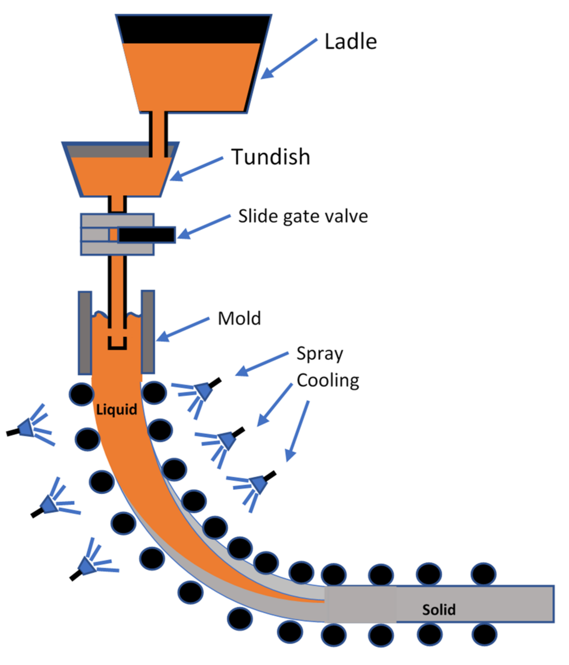
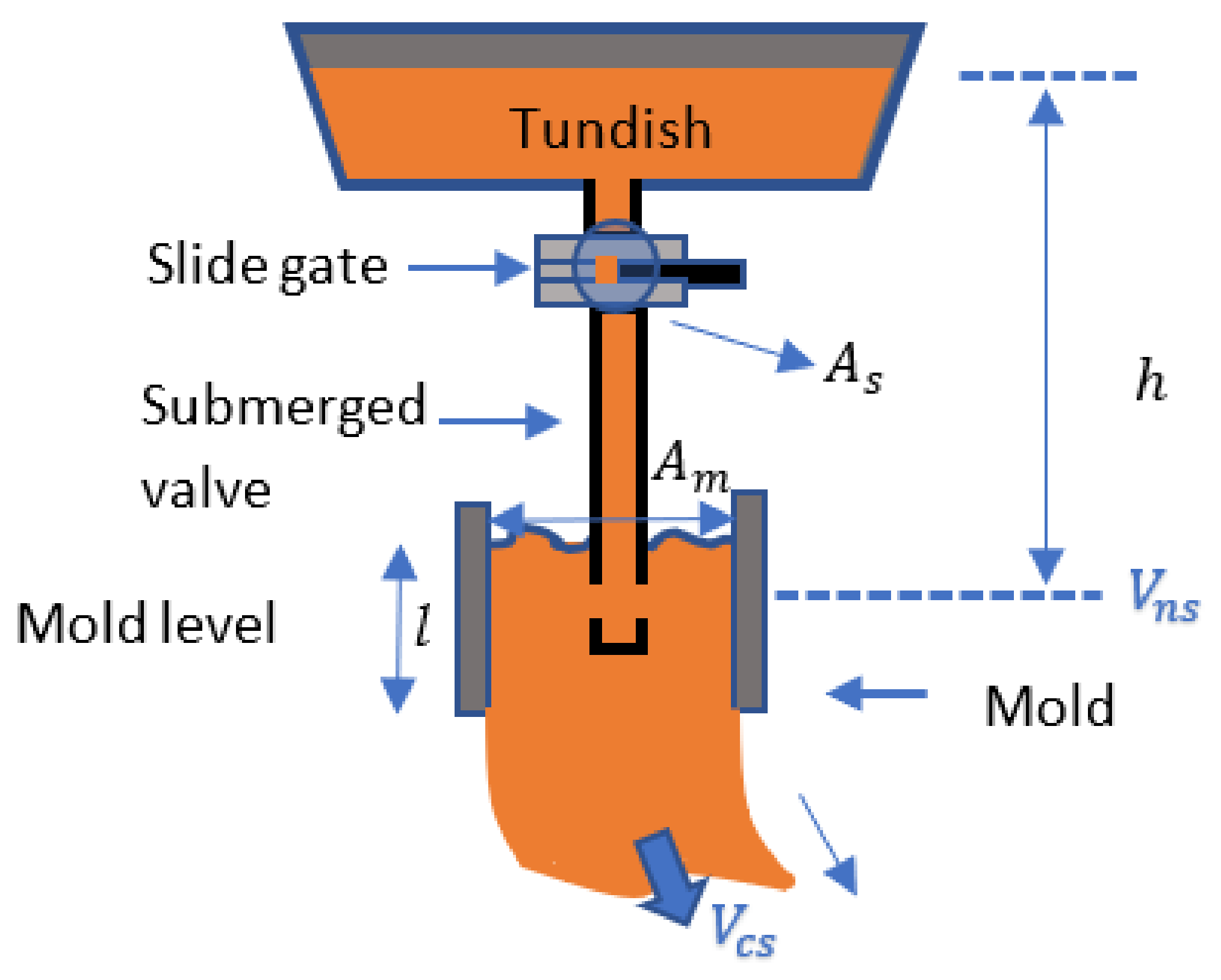
2. Mold Level Process and Disturbances

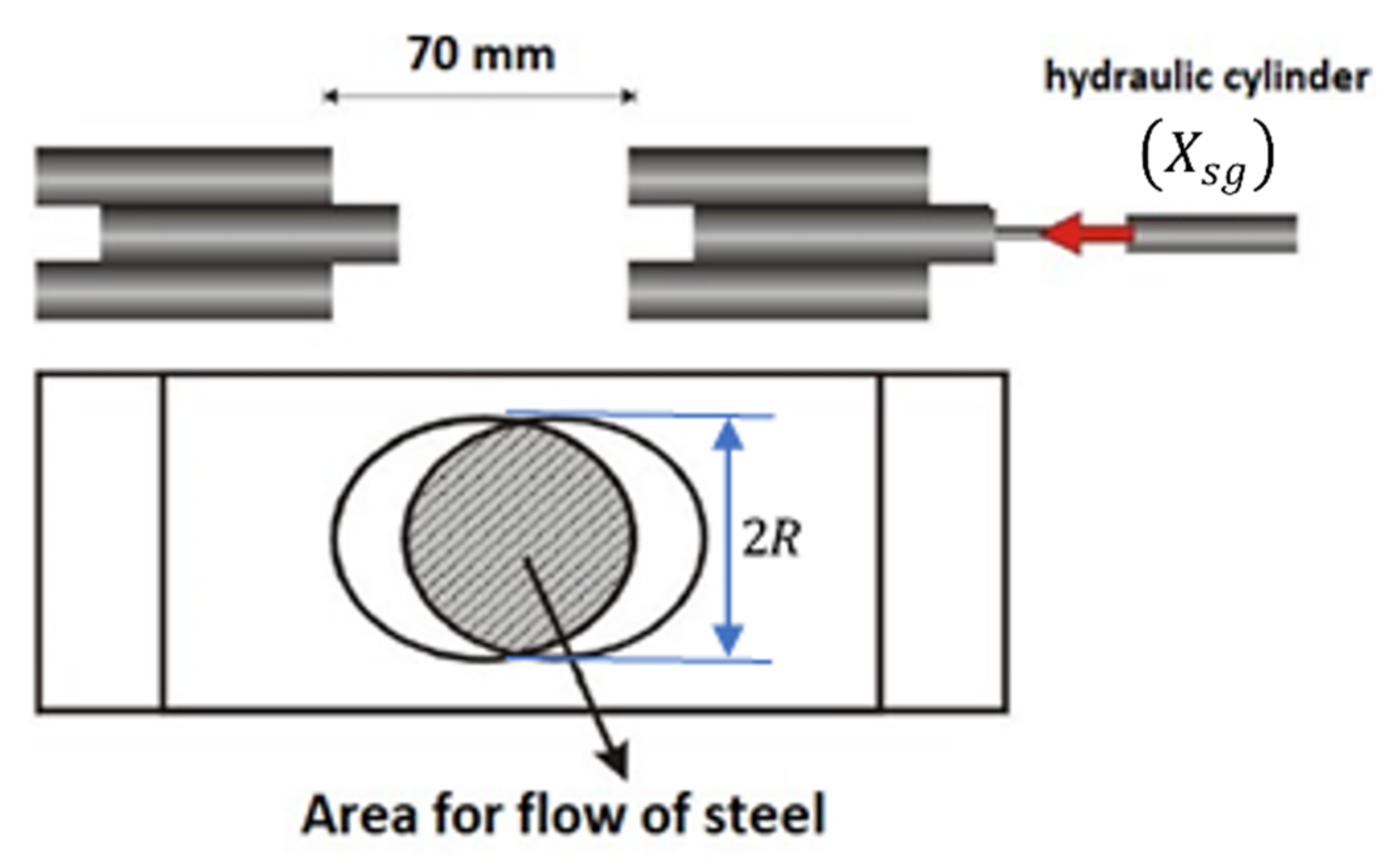
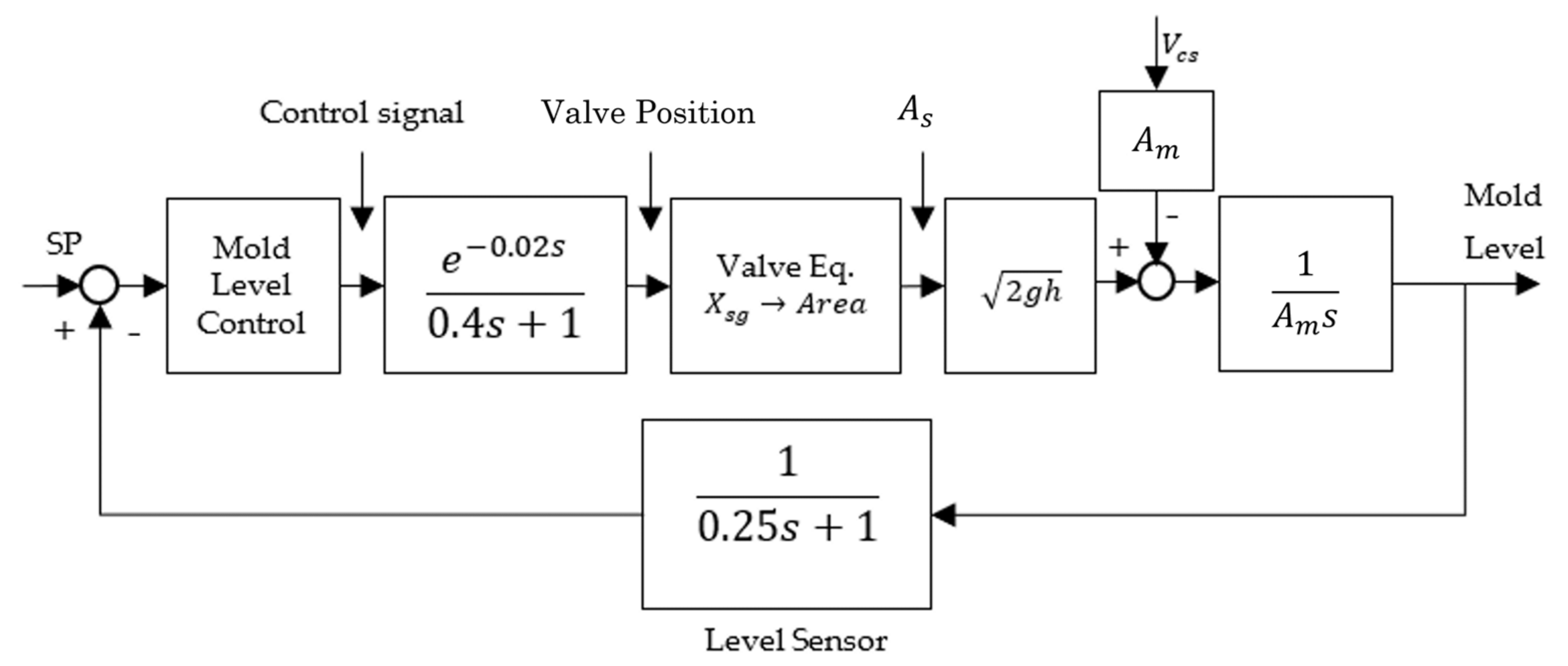
2.1. Nonlinear Modeling of the Mold Level Loop

In this section, the mold level mathematical model is presented, a model that was validated using real data from a steel industry obtained from another study [26].

Figure 2 shows the steel flow from the tundish to the mold. For modeling, it is established that, in a steady-state, the amount of steel that enters the mold must be the same amount as what exits so that the mold level l is kept constant. This process can be shown as follows:

where:

• $V_{ns}$ is the flow of steel into the slide gate valve,
• $V_{cs}$ is the casting speed,
• $A_s$ is the effective slide gate valve area for steel passage,
• $A_m$ is the mold area,
• $l$ is the mold level, and
• $h$ is the distributor height.

Therefore, in a steady-state, the change in the steel volume inside the mold is given by Equation (1).

$$A_m\left(\frac{dl}{dt}\right)=A_s{V}_{ns}-A_m{V}_{cs}$$

(1)

The slide gate valve is located next to the outlet of the tundish and is responsible for transporting the flow of steel into the mold, through the submerged valve. The flow of steel into the slide gate valve according to [5] can be written as $V_{ns}=\sqrt{2gh}$. Thus, from Equation (1), we obtain Equation (2):

$$\left(\frac{dl}{dt}\right)=\frac{1}{A_m}\left(A_s\sqrt{2gh}-A_m{V}_{cs}\right)$$

(2)

The slide gate valve is a device with three overlapping plates that have circular holes with identical radius. The center plate moves horizontally ($X_{sg}$) inside two fixed plates to adjust the openness area for steel flow, defined by the intersection of the circular concentric holes as shown in Figure 3.

The effective steel flow area ($A_s$) in the valve, presented in Equation (3), is calculated considering the intersection of the concentric holes and the displacement of the center plate [26].

$$A_S=2\left[R^2 co{s}^{-1} \left(\frac{R-\frac{X_{sg\left(t\right)}}{2}}{R}\right)-\left(R-\frac{X_{sg\left(t\right)}}{2}\right)\sqrt{R{X}_{sg}-{\left(\frac{X_{sg\left(t\right)}}{2}\right)}^2}\right]$$

(3)

Figure 4 represents the control loop, considering the representation of Equation (2), with the following parameters: $V_{cs}=1.2 \mathrm{m}/\min$, $A_m=\mathrm{250,000} {\mathrm{mm}}^2$, $h$ = 1200 mm, $X_{sg}$ = 35 mm, and R = 35 mm that is the gate valve orifice radius.

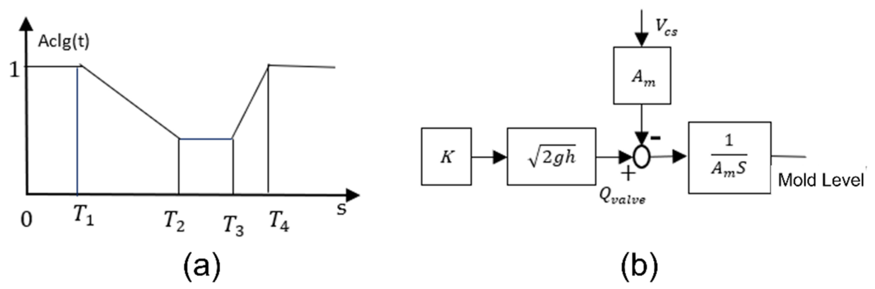
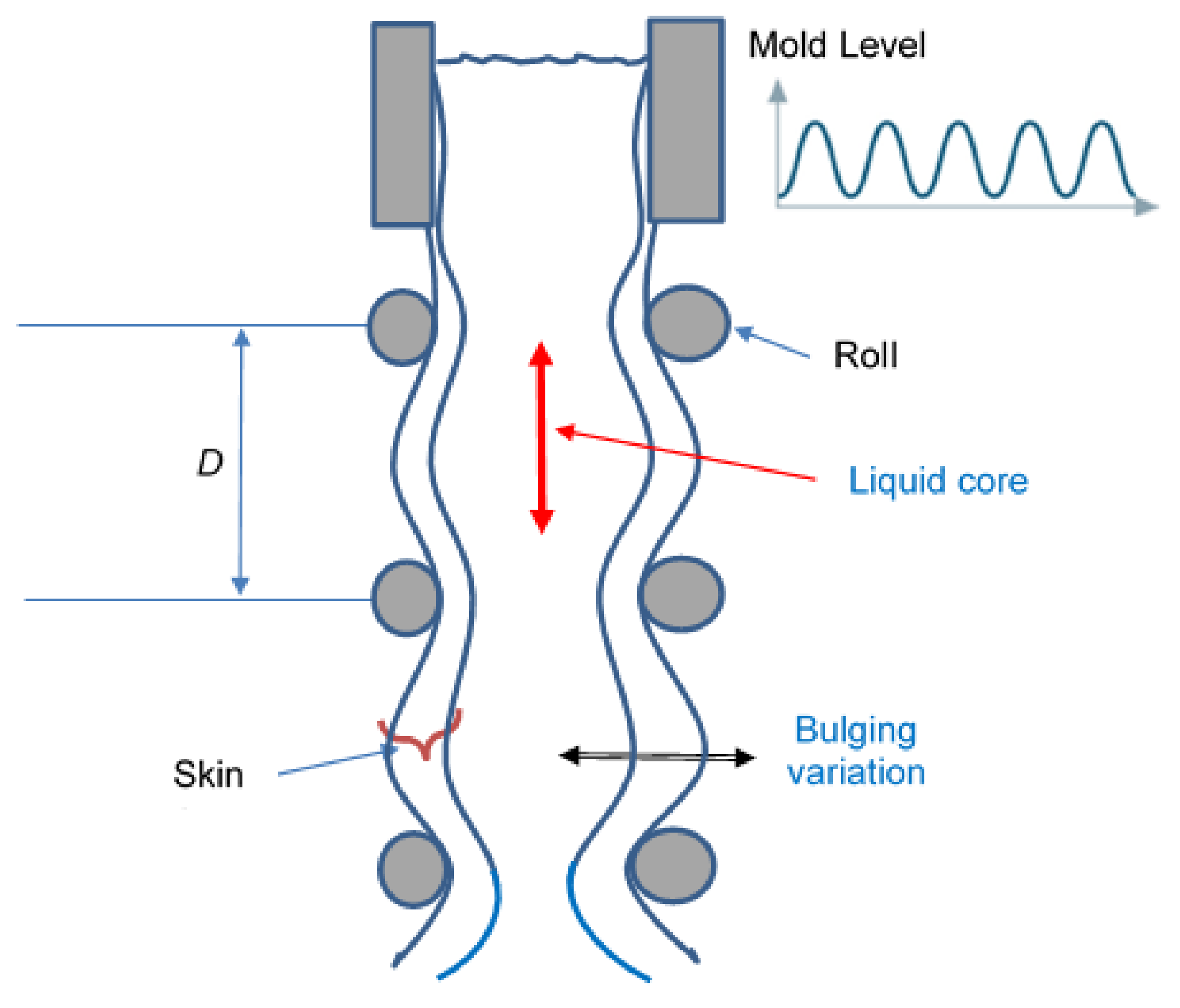
2.2. Bulging Disturbances

In the mold, there is an occurrence of a series of disturbances inherent to the metallurgical process that affect directly and indirectly the stable regime of the level of steel in the mold surface and can be interpreted as disturbances to be controlled or reduced by the control system. The bulging disturbance is similar in shape to a superposition of sinusoidal waves, which cause the mold steel level to oscillate periodically [2]. The bulging disturbance and the consequent variation of the steel level in the mold has the ultimate consequence of emergency defects in the slabs produced by the casting machine as well as the risk of an overflow of steel on the mold and breakouts.

After passing through the mold, the steel slab within the segments (i.e., within the casting machine) has a “skin” in which there is still liquid steel that will gradually be cooled by the addition of water on its surface until it is completely solidified before leaving the machine. This still liquid steel slab exerts a force that tends to push the liquid steel out of the segment, a movement that is impaired by the rollers that comprise the segments, which have a spacing D between them. When passing through the rollers, the slab will simultaneously retract and expand, which is a phenomenon that occurs throughout the machine wherever there is liquid steel inside, which reaches up to the mold. Given that the machine has a speed of casting extraction for the slab inside, called $V_{cs}$, the effect due to the expansion and retraction of the internal board within the machine causes the appearance of sinusoidal waves on the surface of the mold, which can be seen in Figure 5.

These waves are a consequence, therefore, of the changes in the volume of steel inside the segments. The appearance of the bulging phenomenon mainly occurs within the machine, next to the mold, where there is a greater volume of liquid steel within the slab and, obviously, a less thick “skin” of solidified steel. Bulging disturbance is directly related to cooling capacity and speed, the dimensioning of the distance of the rollers, and the type of steel being produced at the casting machine (the lower the amount of carbon in its composition together with the addition of alloys, the greater the amplitude of the phenomenon), among other factors [7,10,26].

Another study [30] presents an overview of the most important perturbations and uncertainties that affect the mold level, stating that bulging disturbance is the most critical disturbance, with harmonics normally up to the sixth order.

The frequency of bulging depends on both the spacing between the respective rolls, where the phenomenon occurs and the speed of extraction. According to [7], the oscillation frequency is approximately determined by Equation (4):

$$f_{oscillation}(H_z)=\frac{V_{cs}\left(\mathrm{m}/\min \right)}{D\left(\mathrm{m}\right) \cdot 60}$$

(4)

2.3. Clogging/Unclogging Disturbances

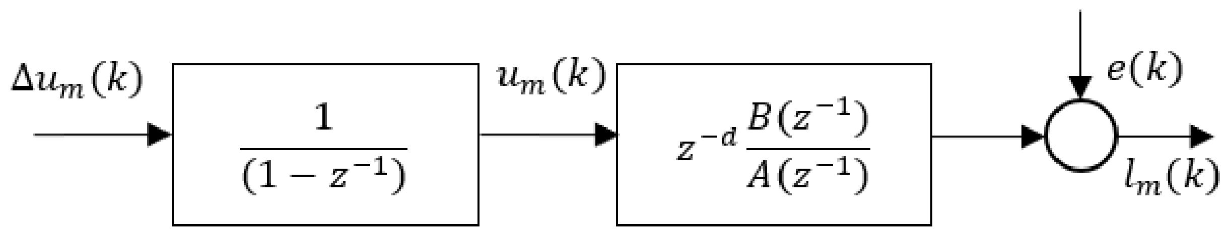
The progressive accumulation or deposition of alumina and other products on the walls of the submerged valve and/or on the gate valve is known as clogging [31,32]. It causes an increasing reduction in the effective passage for liquid steel through the valve. This reduction is compensated by the controller, which regulates the slide gate valve opening. In addition to this effect, the occurrence of an abrupt release of accumulated alumina (unclogging) is quite probable whereby the sudden freeing of the steel flow requires the controller to stabilize the process conditions as quickly as possible.

Observing the position of the gate valve and the mold level in a real plant during a clogging/unclogging disturbance, we concluded that the effective gate valve area is given by $K=A_s·A_{clg}$, where $A_{clg}$ represents the clogging/unclogging rate of the gate valve area, as defined by Equation (5) and illustrated in Figure 6a. When $A_{clg}=1,$ the gate valve area is completely unclogged, and when $A_{clg}=0,$ it is totally clogged. Thus, we can simulate the opening movement on the valve by an increasing random function in time proportional to the gate valve obstruction [26]. After finishing the effect of clogging, the slide gate valve reaches its maximum aperture and stays that way until unclogging (unblocking) occurs a few seconds later. Thus, the simulation of the obstruction in the gate and/or submerged valve area can be performed by multiplying the area of the gate valve ($A_s$) without obstruction by the unclogging rate ($A_{clg}$). Figure 6b is a block diagram showing the clogging/unclogging disturbances.

$$A_{clg}\left(t\right)=\left\{\begin{array}{c}1-{\beta }_1\left(t-T_1\right), T_1\le T_2\\ r_{max}\hspace{1em}\hspace{1em}\hspace{1em}\hspace{1em}\hspace{1em}, T_2\le t<T_3\\ r_{max}+{\beta }_2\left(t-T_3\right), T_3\le t<T_4\end{array}\right.$$

(5)

where $T_1$ is the time when gate valve clogging begins, $T_2$ is the time when the maximum blockage occurs, $T_3$ and $T_4$ are, respectively, the beginning and end instants of the unblocking process, and $r_{max}$ is the maximum reduction factor such that $0<r_{max}<1$ and $r_{max}=1-{\beta }_1\left(T_2-T_1\right)=1-{\beta }_2\left(T_4-T_3\right)$. The variable ${\beta }_1$ defines the clogging speed and ${\beta }_2$ the unclogging speed. Based on practical observations of the real plant where the modeling data were obtained, we can state that the time intervals in Figure 6a are $20 \mathrm{s}<(T_2-T_1)<120 \mathrm{s}$, $10 \mathrm{s}<(T_3-T_2)<60 \mathrm{s},$ and $0 \mathrm{s}<(T_4-T_3)<5 \mathrm{s}$.

3. The Controllers

The repetitive structure used in this work, as shown in Figure 7, has been used by other researchers [28,33] to combine a GPC controller in the direct loop and a repetitive GPC (R-GPC) with an N-periodic internal model in the feedback. Reference tracking is ensured by the GPC controller, which generates the control signal, $u_m\left(k\right)$, for the process and the model. The model output signal $l_m\left(k\right)$ feeds back to the GPC controller to detect changes in the reference signal $w\left(k\right)$, thus generating the error, which is inserted into the GPC controller. The disturbance of the periodic signal and/or the modeling error is handled by the R-GPC controller, through the $l_{rp}\left(k\right)$ signal, given by $l_{rp}\left(k\right)=l\left(k\right)-l_m\left(k\right)$. If there is no disturbance signal ($d\left(k\right)$) or modeling error, then $l_{rp}\left(k\right)=0$, and the closed-loop control system operates with only the GPC controller. If $l_{rp}\left(k\right)$ is different from zero, the R-GPC controller starts to act in the control loop to maintain $l_{rp}\left(k\right)$ equal or close to zero, reducing undesirable disturbance signals and modeling errors. The control signal applied to the process $u\left(k\right)$ is given by $u\left(k\right)=u_m\left(k\right)+u_{rp}\left(k\right)$.

3.1. The GPC

The GPC controller requires a CARIMA model given by:

$$A\left(z^{-1}\right)l_m\left(k\right)=z^{-d}B\left(z^{-1}\right)u_m\left(k-1\right)+\frac{e\left(k\right)}{\Delta }$$

(6)

where $\Delta =\left(1-z^{-1}\right); A\left(z^{-1}\right)$ and $B\left(z^{-1}\right)$ are polynomials of orders $n_a$ and $n_b$, respectively; and e(k) is a zero-mean white noise. The GPC control law is determined by minimizing the following cost function:

$$J_{GPC}={\displaystyle \sum }_{j=N_1}^{N_2}\delta {[{\widehat{l}}_m\left(k+j|k\right)-w\left(k+j\right)]}^2+{\displaystyle \sum }_{j=1}^{N_u}\lambda {[{\Delta \mathrm{u}}_m\left(k+j-1\right)]}^2$$

(7)

where $\delta$ and $\lambda$ are weighting factors in the error and control signals, respectively; $N_1$ and $N_2$ are the minimum and maximum prediction horizon of output, respectively; and N_u is the control horizon. The terms ${\widehat{l}}_m\left(k+j\right)$ and $w\left(k+j\right)$ represent the predictions of mold level and reference signals j steps ahead, and $\Delta u_m\left(k\right)={\mathrm{u}}_m\left(k\right)-u_m\left(k-1\right)$ is the control signal variation or incremental action that must be integrated to determine the control action ${\mathrm{u}}_m\left(k\right),$ to be applied in the mold level plant (see Figure 8).

The unconstrained minimization of $J_{GPC}$ with respect to $\Delta u_m\left(k\right),$ shown in [19], is given by:

$${\Delta \mathrm{u}}_m\left(k\right)=K_{GPC}\left(w-f\right)$$

(8)

where $K_{GPC}$ is a gain that depends on the CARIMA model, $f$ is the free response, and $w$ is a reference as defined in [19]. The applied control signal is $u_m\left(k\right)=\Delta u_m\left(k\right)+u_m\left(k-1\right)$.

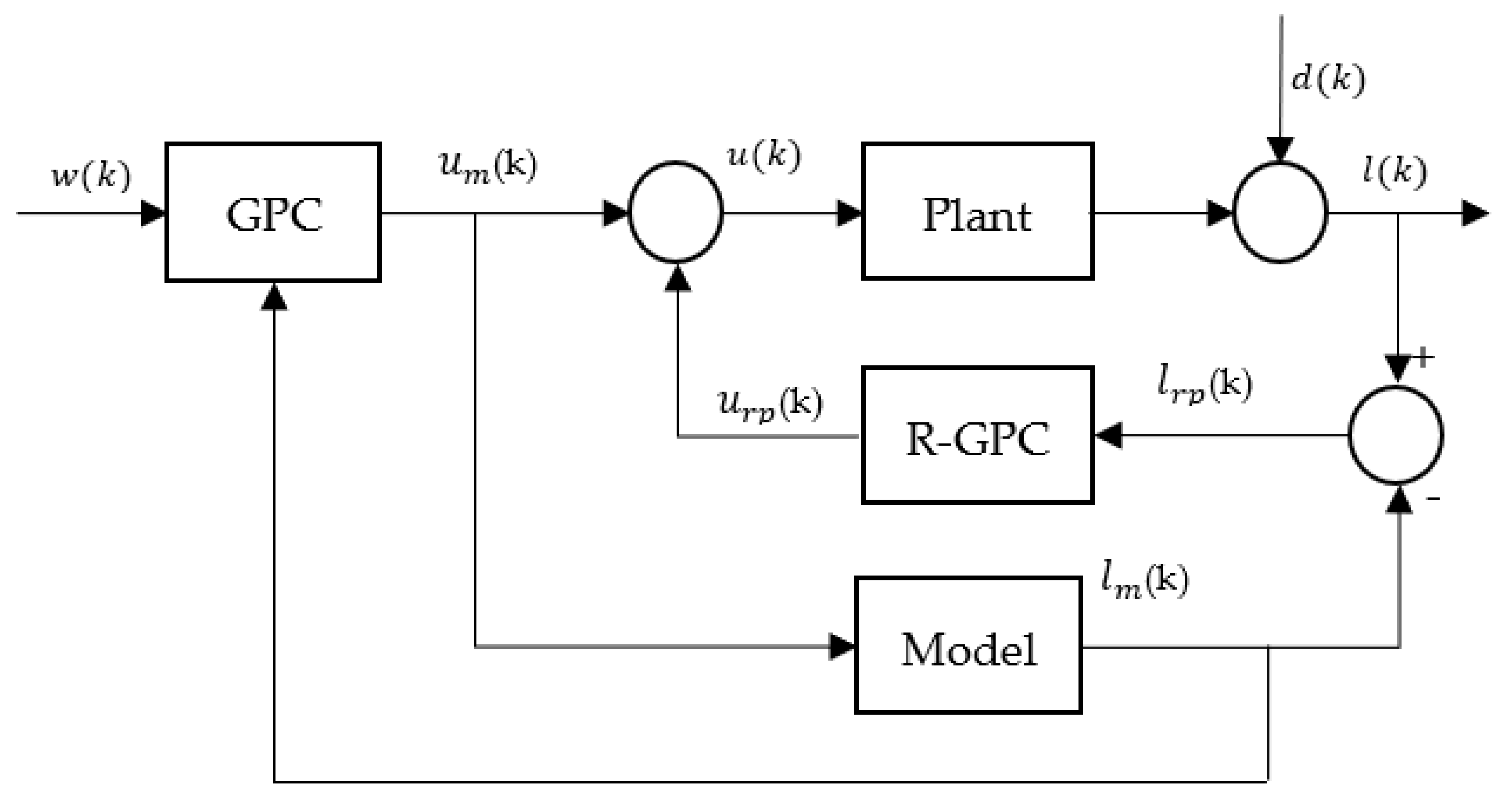
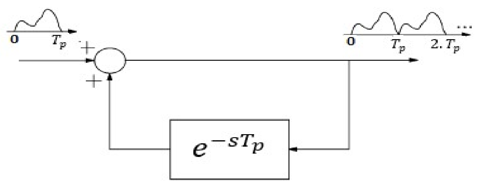
3.2. Repetitive Generalized Predict Controller (R-GPC)

The repetitive controller (RC) uses the principle of the internal model and follows the internal model of the periodic signal generator [34]. This principle states that, if a certain signal must be tracked or rejected without steady-state error, the generator must be inside the controller or in the plant itself [35].

A periodic signal $r\left(t\right)$ with period $T_p$ can be represented in Fourier series [35], as shown in Equation (9).

$$r\left(t\right)={\displaystyle \sum }_{n=-\infty }^{\infty }{a}_n{}^{-j\frac{2\pi nt}{T_p}}$$

(9)

and its transfer function using Laplace is:

$$R\left(s\right) = \frac{1}{s}{\displaystyle \prod }_{n=1}^{\infty }\frac{{\left(\frac{2\pi n}{T_p}\right)}^2}{s^2+{\left(\frac{2\pi n}{T_p}\right)}^2} = \frac{T_p e^{\frac{-s{T}_p}{2}}}{1-e^{-s{T}_p}}$$

(10)

The term $T_p·e^{\frac{-s{T}_p}{2}}$ is a delay with a gain $T_p$; therefore, it will be enough to include $\frac{1}{1-e^{-s{T}_p}}$ inside the control loop to reproduce the periodic signal. Thus, Equation (10) can be considered positive feedback with a delay, as shown in Figure 9.

The Z transform of a pure delay $e^{-sT}$ is $z^{-N}$, where $N$ is the integer multiple of the sampling period, $T_s$, such that $N=\frac{T_p}{T_s}, N\in Z_{+}^{*}$. Thus, the discrete internal model is represented by:

$$I_M\left(z\right)=\frac{1}{1-Z^{-N}}$$

(11)

$I_M\left(z\right)$ augments the system with all poles necessary to reproduce desirable periodic signals and needs to be chosen considering $T_p=N\cdot T_s$ [29].

As a repetitive controller (RC), the N-periodic internal model (11) is used in R-GPC, therefore it is necessary to insert it in series with the CARIMA model (6), thus we obtain:

$$A\left(z^{-1}\right)l_{rp}\left(k\right)=z^{-d}B\left(z^{-1}\right)u_{rp}\left(k-1\right)+\frac{e\left(k\right)}{{\Delta }^N}$$

(12)

where ${\Delta }^N=1-z^{-N}$. The repetitive N-periodic internal model in series with the mold level plant is shown in Figure 10.

The R-GPC control law is determined by minimizing the cost function given by Equation (13):

$$J_{RGPC}\left(k\right)={\displaystyle \sum }_{j=N_1}^{N_2}\delta {[{\widehat{l}}_{rp}\left(k+j|k\right)]}^2+{\displaystyle \sum }_{j=1}^{N_{u_{rp}}}{\lambda }_{rp}{[{\Delta }^N{u}_{rp}\left(k+j-1\right)]}^2$$

(13)

The repetitive internal model in its pure form, given by Equation (11), has infinite gain in harmonic frequencies of the periodic signal. This makes the closed-loop system very susceptible to measurement of noise and modeling errors because these elements usually are influenced by terms of high frequencies. So, it is necessary to add a filter that compensates for this problem, and, in this way, ${\Delta }^N$ is changed to ${\Delta }^{Nf}=1-H\left(z\right) · z^{-N}$, where, in this work, the low-pass FIR filter $H\left(z\right)$ is given by Equation (14):

$$H\left(z\right)=q_{1}z+q_0+q_1{z}^{-1}$$

(14)

where $0<q_0<1$ and $q_1=\frac{\left(1-q_0\right)}{2}$.

The filter shown in Equation (14) has null phase and unit gain to attenuate the gains of harmonics at high frequencies without dislocating its phase [35]. This is an effective feature for systems that have a repetitive loop because, if a filter that modifies the phase of the system is used, all gains present in the harmonics will be displaced, altering the learning and reproduction capacity of the periodic signal.

To define the internal model with a filter in the system, the CARIMA model is modified again as follows:

$$A\left(z^{-1}\right)l_{rp}\left(k\right)=z^{-d}B\left(z^{-1}\right)u_{rp}\left(k-1\right)+\frac{e\left(k\right)}{{\Delta }^{Nf}}$$

(15)

In this way, the R-GPC control law with filter is determined by minimizing the cost function (13), $\Delta$ by ${\Delta }^{Nf}$ as shown in Equation (16).

$$J_{RGPC}={\displaystyle \sum }_{j=N_1}^{N_2}\delta {[{\widehat{l}}_{rp}\left(k+j|k\right)]}^2+{\displaystyle \sum }_{j=1}^{N_{u_{rp}}}{\lambda }_{rp}{[{\Delta }^{Nf}{u}_{rp}\left(k+j-1\right)]}^2$$

(16)

In a real process, constraints are a result of field equipment limitations (such as hydraulic/electrical capacity for moving actuators, stroke limitation for valves, and tank capacity) [19]. In this work, the constraints on the control signal $u\left(k\right), \mathrm{as} \mathrm{well} \mathrm{as} \mathrm{on} \mathrm{the} \mathrm{output} \mathrm{signal} l\left(k\right),$ and its slew rate $\Delta u_{rp}\left(k\right)$ will be considered. In predictive controllers, constraints can be inserted inside the controller, and, when considered, there is no explicit solution for the cost function. Thus, the quadratic programming problem must be solved, requiring the use of specific routines for the ${\Delta }^{Nf}{u}_{rp}\left(k\right)$ calculation. Constraints can be written in the form of matrix inequalities considering the matrices and vectors $\mathit{I}$, ${\mathit{S}}_{\mathbf{0}}$, $\mathit{G}$, ${\mathit{u}}_{\mathit{m}\mathit{a}\mathit{x}}$, ${\mathit{u}}_{\mathit{m}\mathit{i}\mathit{n}}$, ${\mathit{I}}_{\mathit{m}\mathit{a}\mathit{x}}$, ${\mathit{I}}_{\mathit{m}\mathit{i}\mathit{n}}$, ${\mathit{c}}_{\mathbf{0}}$, ${\mathit{y}}_{\mathit{m}\mathit{a}\mathit{x}}$ and ${\mathit{y}}_{\mathit{m}\mathit{i}\mathit{n}}$ according to [29] and inserted into the optimization problem within the controller algorithm. In this work, the inequality must be written as a function of ${\Delta }^{Nf}{u}_{rp}\left(k\right)=u_{rp}\left(k\right)-u_{rp}\left(k-N\right)$, as it is the decision variable of the cost function. Thus, the optimization problem in the presence of constraints is determined by solving the following mathematical problem:

$$\underset{{\Delta }^{\mathit{N}\mathit{f}}{\mathit{u}}_{\mathit{r}\mathit{p}}}{min}{J}_{RGPC}\hspace{1em}sa\hspace{1em}{\mathit{A}}_{\mathit{i}\mathit{n}\mathit{e}\mathit{q}}{\Delta }^{\mathit{N}\mathit{f}}{\mathit{u}}_{\mathit{r}\mathit{p}}\le {\mathit{b}}_{\mathit{i}\mathit{n}\mathit{e}\mathit{q}}$$

(17)

where:

$$A_{ineq}={\left[\begin{array}{c}\mathit{I}\\ -\mathit{I}\\ {\mathit{S}}_{\mathbf{0}}\\ -{\mathit{S}}_{\mathbf{0}}\\ \mathit{G}\\ -\mathit{G}\end{array}\right]}_{\left(4N_u+2N_2\right)X{N}_u}$$

and

$${\mathit{b}}_{\mathit{i}\mathit{n}\mathit{e}\mathit{q}}={\left[\begin{array}{c}{\mathit{u}}_{\mathit{m}\mathit{a}\mathit{x}}-{\mathit{u}}_{\mathit{r}\mathit{p}}\left(k-N\right)\\ -{\mathit{u}}_{\mathit{m}\mathit{i}\mathit{n}}+{\mathit{u}}_{\mathit{r}\mathit{p}}\left(k-N\right)\\ {\mathit{I}}_{\mathit{m}\mathit{a}\mathit{x}}+{\mathit{c}}_{\mathbf{0}}{\Delta }^N{u}_{rp}\left(k-1\right)-\Delta {\mathit{u}}_{\mathit{r}\mathit{p}}\left(k-N\right)\\ {\mathit{I}}_{\mathit{m}\mathit{i}\mathit{n}}-{\mathit{c}}_{\mathbf{0}}{\Delta }^N{u}_{rp}\left(k-1\right)+\Delta {\mathit{u}}_{\mathit{r}\mathit{p}}\left(k-N\right)\\ {\mathit{y}}_{\mathit{m}\mathit{a}\mathit{x}}-\mathit{f}\\ -{\mathit{y}}_{\mathit{m}\mathit{i}\mathit{n}}+\mathit{f}\end{array}\right]}_{\left(4N_u+2N_2\right)X1}$$

The applied control signal is $u_{rp}\left(k\right)={\Delta }^N{u}_{rp}\left(k\right)+u_{rp}\left(k-1\right)$.

As shown in Figure 7, the control action applied in the process will be given by $u\left(k\right)$ = $u_m\left(k\right)+u_{rp}\left(k\right)$, where $u_m\left(k\right)$ is the action responsible for reference tracking and $u_{rp}\left(k\right)$ is the action responsible for rejecting disturbances. This form of implementation avoids the occurrence of interference between the incremental and repetitive models. So, it allows the control structure to obtain different dynamics characteristics to follow references and reject disturbances.

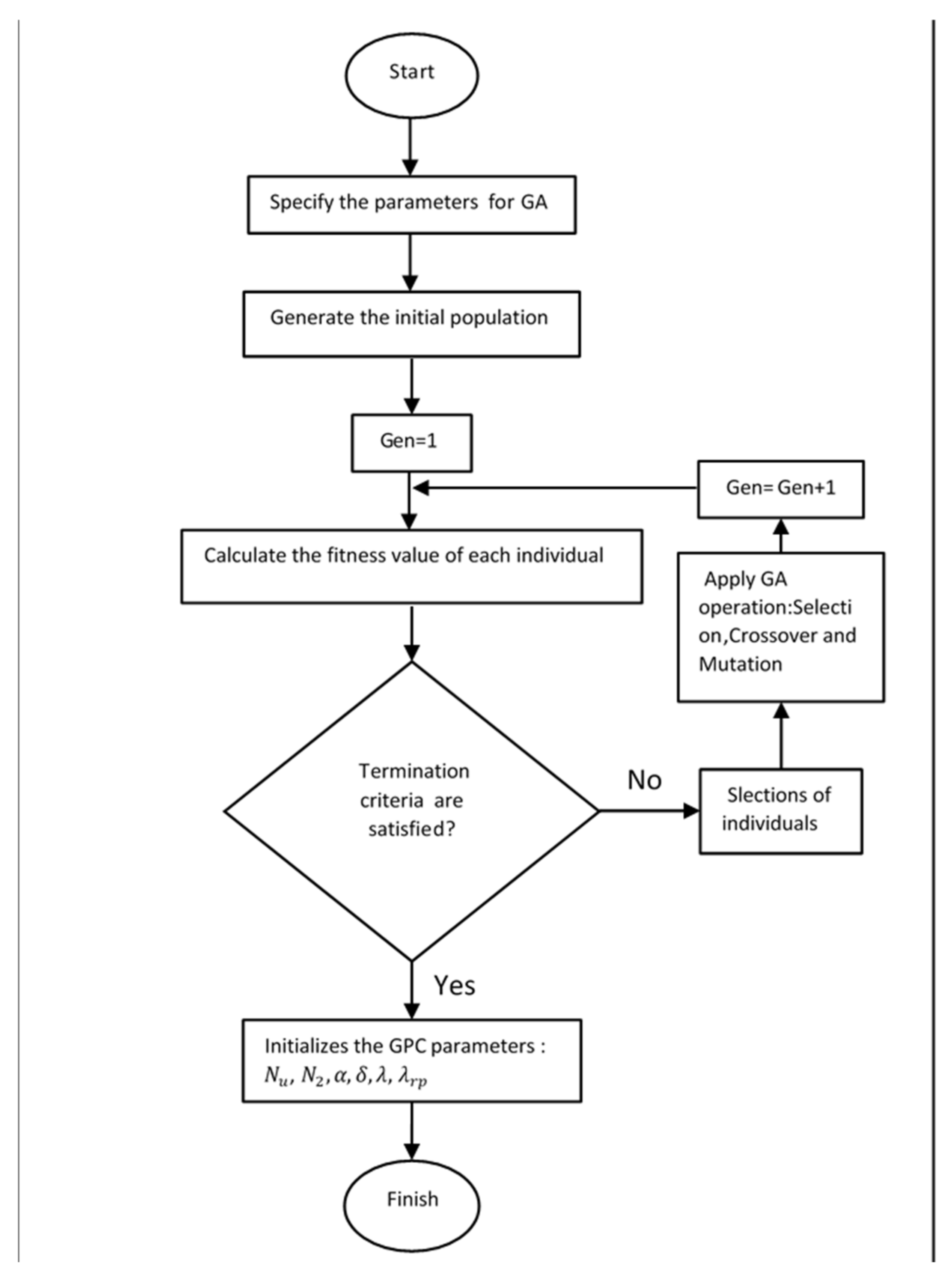
3.3. The Genetic Algorithm (GA)

The good performance of the R-GPC controller is obtained only if the tuning parameters prediction horizon ($N_2$), control horizon ($N_u$), the weighting of the prediction error (δ), suppression factor (λ), constant of the reference trajectory (α), and periodic signal suppression factor (${\lambda }_{rp}$) are properly defined by the designer. In general, the tuning is performed through heuristics, based on trial and error, and is viable only in the predictive controller tuning of processes that have stable behavior in open loops. However, in cases where the process is unstable in open loops (as the level of the continuous casting mold), this procedure is difficult and may not obtain a stable response in a closed-loop or if the controller performance is below expectations. As far as we know, the existing tuning guidelines in the literature do not include the ${\lambda }_{rp}$ parameter. So, the repetitive structure will be tuned by a Genetic Algorithm.

The execution of the GA is performed as follows: First, the process model must be provided. Then, the necessary parameters for the execution of the GA must be defined, such as population size (M), the number of generations (G), crossover rate, and mutation rate, and the type of fitness function and the criterion of selection must be considered. Afterward, M individuals are randomly created by a GA, according to [18]:

$$[N_u,N_2,\alpha ,\delta ,\lambda ,{\lambda }_{rp}]$$

(18)

Then, each individual is applied, in simulation, within the repetitive structure algorithm to control the process and calculate the fitness of each individual within the initial population. Through the fitness function in Equation (19), individuals are classified in descending order, from the best to the worst.

$$Fit(N_u,N_2,\alpha ,\delta ,\lambda ,{\lambda }_{rp})=\frac{1}{\sum {\left(\mathrm{l}-w\right)}^2}$$

(19)

where $l$ is the output of the process and $w$ is the reference.

Following, the GA selects the best individuals through the roulette method, where, using Equation (19), the portion that the individual will have inside the roulette is determined. To select individuals, (M − 1) roulette runs are made. Parallel to roulette selection, the elitism technique is used, where the best individual of each generation is copied directly to the next generation. After the selection process, genetic operations (crossover and mutation) will be performed, in which new individuals will be generated to compose the population of the next generation.

The GA will run a loop of G generations, and, at the end of the last one, it presents the best individual, containing the parameters of the best tuning, which must be effectively applied in the control of the plant. The flowchart of GA is shown in Figure 11.

4. Obtaining the Linear CARIMA Model

The CARIMA model was determined from identification of the mathematical model given in Section 2.1, by considering a random input $u\left(t\right)$, satisfying the following operational conditions: maximum variation of the gate valve opening is equal to $70 \mathrm{mm}$; the height of the tundish is equal to h = 1200 mm; the operational position of the gate valve $X_{sg}=35 \mathrm{mm}$ when the casting speed equals 1.2 m/min. The sample time used in the simulation was 0.12 s.

Figure 12 shows the set of input–output data determined that was used for identification of the mold level model. It was separated into two subsets: training data and validation data.

Applying these data in the Identification Toolbox of MATLAB and using the least square method, many CARIMA models were generated with different orders representing the linear model. After this, Akaike’s Information Criterion and the Final Prediction Criterion were used to select the best model [36].

The selected model has orders $n_a=2$ and $n_b=0$ and $d=0$, according to the following discrete Equation (20):

$$l\left(t\right)=1.822 l\left(t-1\right)-0.822 l\left(t-2\right)+0.01924 u\left(t-1\right)$$

(20)

The comparison between the prediction made by the identified model 20 steps ahead, with the simulation of the mold level process determined from Section 2.1, presented a 97.9% fitness rate. Therefore, we concluded that the model is sufficient to represent the mold level process and in simulations.

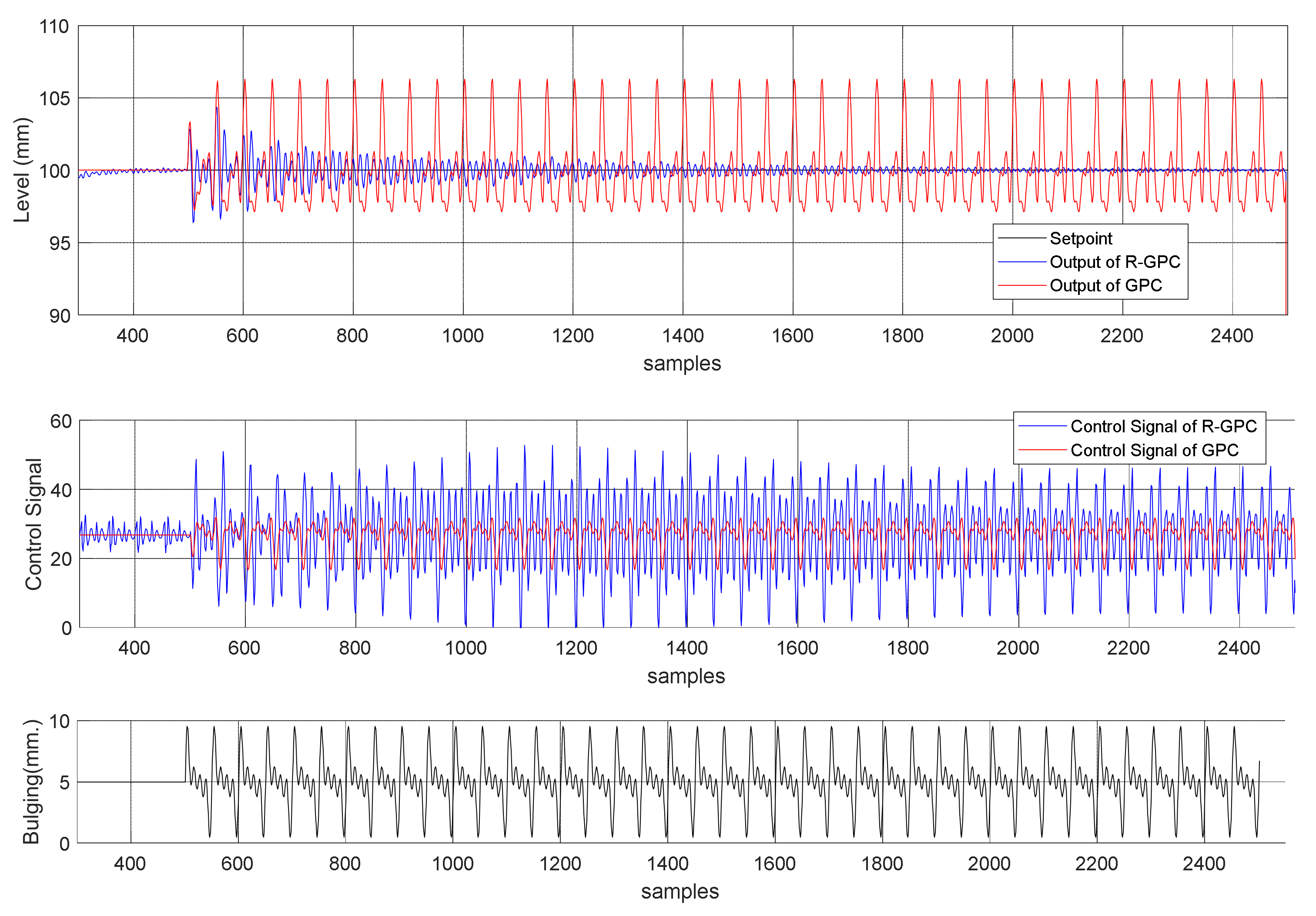
5. Numerical Results

The repetitive structure with constraints will be applied in a mold level simulator that represents a real plant when it is affected by the bulging, clogging/unclogging disturbances and variations in casting speed. In Section 5.1, specifically, the tests will be carried out comparing GPC with constraints with the repetitive structure.

For this, the reference mold level was set to 100 mm, and the bulging signal consisted of sine waves with an amplitude of approximately 10.0 mm, peak to peak. It will be considered a more severe bulging effect, so a larger casting speed and a smaller roll spacing will be considered, which, according to Equation (4), causes a higher frequency and makes it even more difficult to control the level.

Thus, the velocity of the casting machine should be V_cs = 2.0 m/min (the maximum capacity of the machine), and it was considered the smallest physical roller spacing of the real plant from which the model was obtained, which is D = 200 mm. Therefore, the bulging frequency is given by:

$$f_{bulging}\left(hz\right)=\frac{2.0 (\mathrm{m}/\min )}{0.2\left(\mathrm{m}\right) \cdot 60}=0.167 \mathrm{Hz}$$

(21)

To simulate the bulging disturbance as accurately as possible, harmonics of the bulging signal were added with values 2, 3, and 4 times higher than the bulging fundamental frequency.

To test the controller robustness, variations in the casting speed would be made, which would cause changes in both the plant model and the bulging frequency.

The range of variation of the casting speed would be from 0.6 m/min to 2.0 m/min, complying with the operating range of the industrial plant modeled.

All controllers were tuned using a GA. The tests were performed with process constraints entered within the predictive control.

5.1. Comparison between GPC and Repetitive Structure

In this section, we will make a comparison of the efficiency using the GPC controller and the repetitive structure when the process has periodic disturbances.

The tuned parameters for each controller can be seen below:

-

GPC: N_u = 5, N₂ = 5, α = 0.92, δ = 270.95, and λ = 420.66

-

Repetitive structure: N_u = 8, N₂ = 9, α = 0.98, δ = 712.69, λ = 297.35, and ${\lambda }_{rp}$ = 62.04

The response presented by the GPC algorithm and the repetitive structure can be seen in Figure 13.

According to the level graph of Figure 13, the GPC was not efficient enough to reject the bulging disturbance; the oscillation around the setpoint of the mold level (100 mm) was from 97 mm to 107 mm with a maximum amplitude of 10 mm, which was inside the disturbance amplitude range. Therefore, the GPC was not able to reduce the disturbance, which caused an oscillation in the mold level. Using the repetitive structure, this oscillation was between 99.95 mm and 100.1 mm, with a maximum amplitude of 0.15 mm, which is low compared with the maximum amplitude of the disturbance. Therefore, the repetitive structure was able to reduce the disturbance by around 98.5%. This happened because the R-GPC controller can reject periodic disturbances. Due to these results, all tests from now on will be made using only the repetitive structure.

The graph of the control signal in Figure 13 presents the control signal applied for both controllers. It is observable that the control signal presented by the repetitive structure shows a smaller oscillation since it has incorporated the disturbance rejection, which does not happen with the GPC. The bulging graph in Figure 13 represents the bulging disturbance. The fundamental frequency of the bulging disturbance was 0.167 Hz, and it had four harmonics. The disturbance was applied starting with the 500th sample.

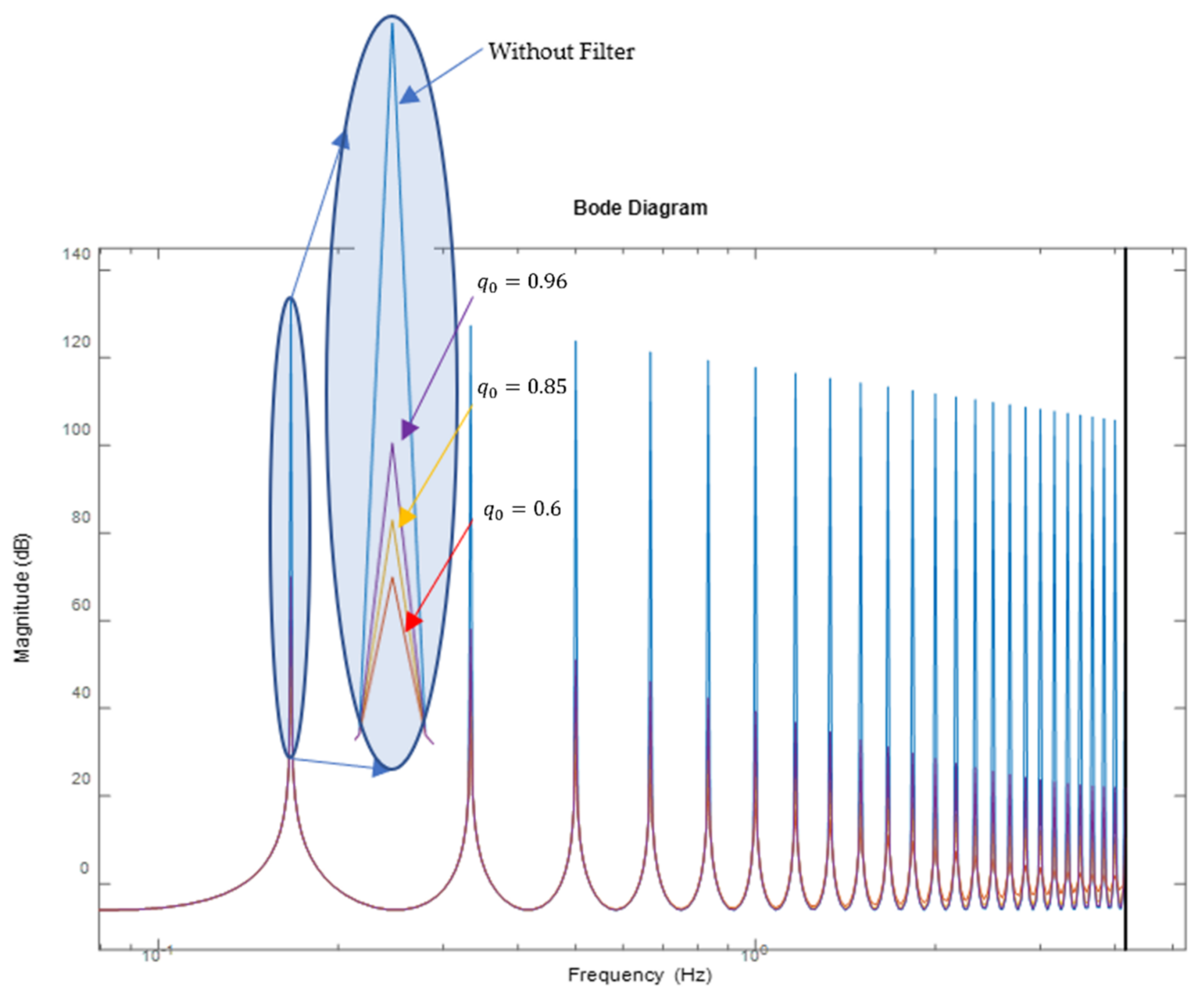
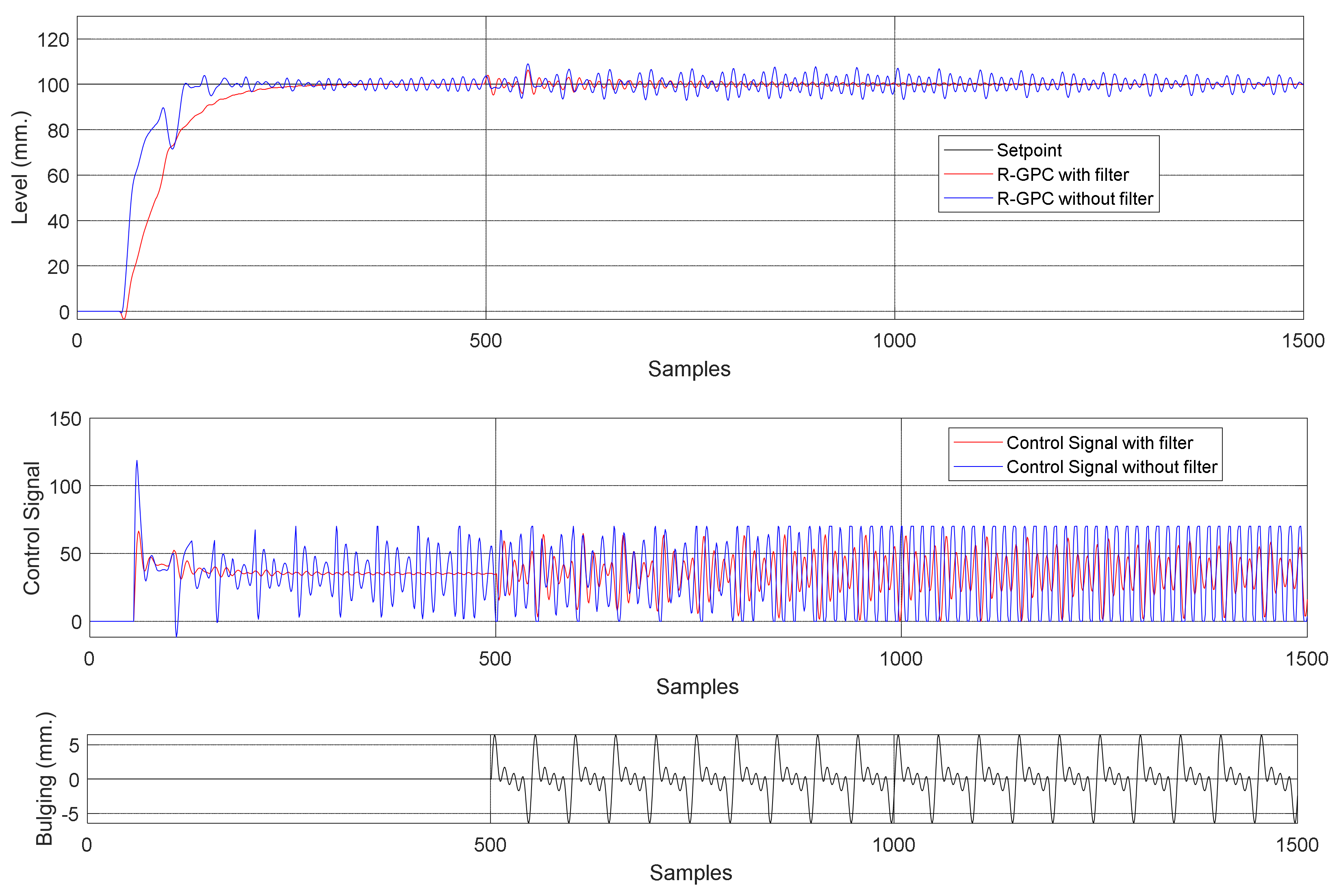
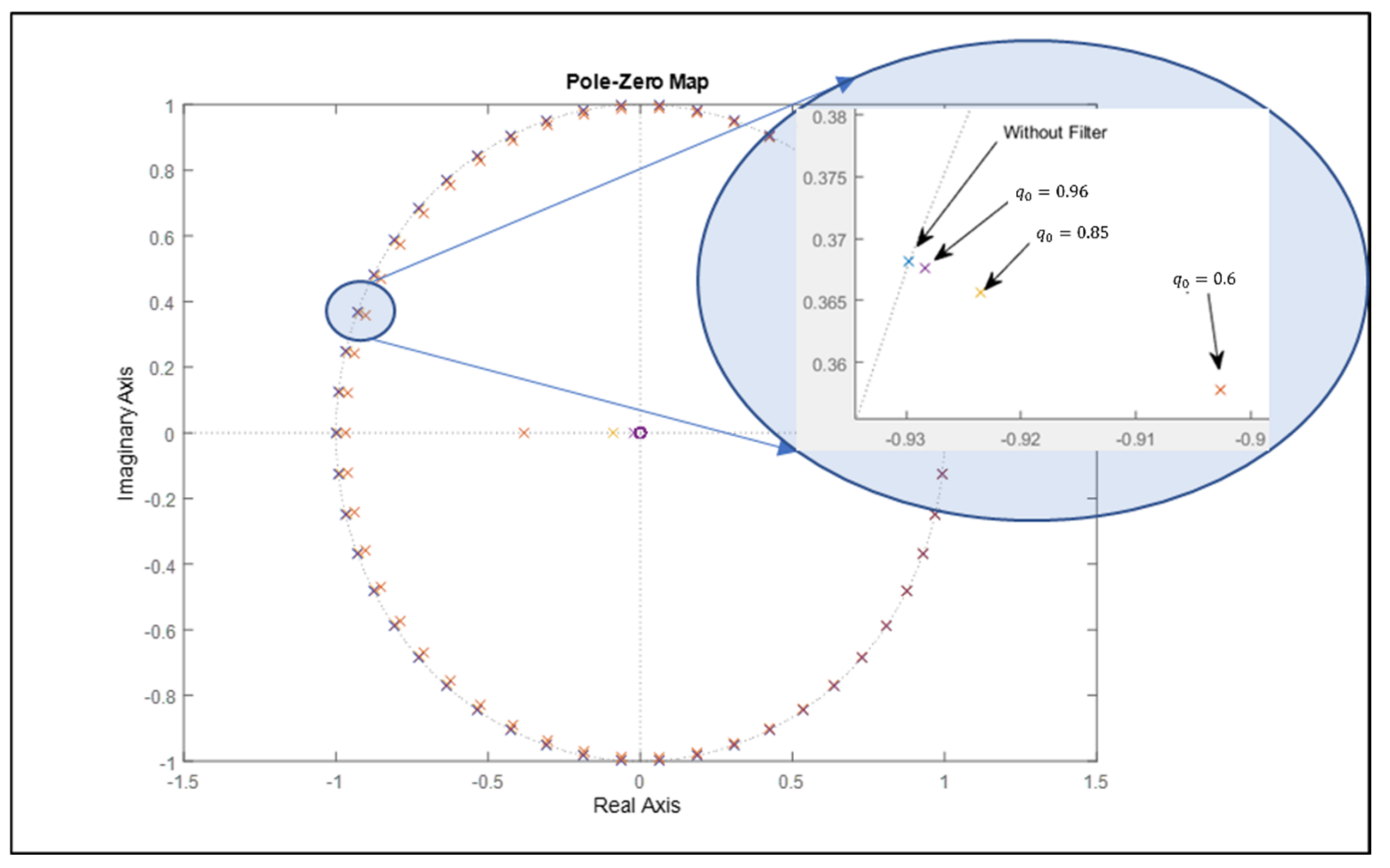
5.2. Comparison between the Repetitive Structure with and without a Filter

In this section, the performance of the repetitive structure, shown in Figure 7, with and without filtering for processes with disturbances of bulging and clogging/unclogging and variations in the casting speed are compared.

The parameters of the repetitive structure with a filter were the same as those presented in Section 5.1. The parameters for the repetitive structure without a filter are N_u = 5, N₂ = 9, α = 0.93, δ = 944.79, λ = 167.17, and ${\lambda }_{rp}$ = 106.22.

The tuning made for this test was for the bulging frequency of 0.167 Hz, with a sampling time of 0.12 s and consequently with N = 50 samples. Therefore, the internal model of R-GPC without a filter is given by $I_M\left(z\right)=\frac{1}{1-z^{-50}}$, and for the R-GPC with filter $I_{Mf}\left(z\right)=\frac{1}{1-0.075 z^{-49}-0.85 z^{-50}-0.075 z^{-51}}$ for $q_0=0.85$, so $q_1=0.075$, according to Equation (14). These same parameters will be used for all simulations of mold level control with disturbances.

The filter choice was made by trial and error. In the first moment, we started with a small value of $q_0$ ($q_0=0.6$), and this value was incremented gradually. The final value of $q_0$ was defined considering the attenuation of the harmonics and the pole displacement for stability, as shown in Figure 14 and Figure 15. However, adding the filter modifies the internal model since, as $q_0$ gets smaller, it makes a higher attenuation of the harmonics, modifying the internal model. Although the system becomes more stable, the capacity of correctly producing the signal that should be rejected is harmed, thus, reducing the capacity of rejecting the disturbance, depending on the filter value. In Figure 14, it is possible to observe the Bode diagram of the internal model without filter and with the adjusted filter; it is shown that the gains in the harmonics of the model without filter are higher than the gains of the model with filter.

Observing the pole placement in Figure 15, it is clear that the model without a filter has the poles located on the unitary circle, while the model with a filter has the poles slightly displaced toward the center of the unitary circle. Therefore, the displacement of the model with a filter helps with stability and robustness.

5.2.1. Process Simulation with Bulging Disturbance

The bulging disturbance was applied in our test, starting in the 500th sample. Figure 16 shows that the amplitude reduction in the bulging by the repetitive structure with a filter was around 98.5%, as shown in Section 5.1. However, the repetitive structure without a filter showed an oscillation from 95.46 mm to 102.9 mm, which means a variation of 7.44 mm, or a reduction of 25.6%, compared with the 10 mm amplitude bulging disturbance. The small reduction using the structure without filter occurred because its control signal was limited by the controller so as not to exceed process constraints.

The control signal shown in Figure 16 presented by the repetitive structure with a filter was softer than the repetitive structure without a filter, directly affecting the slide gate life span.

Some studies, such as [37,38], used as a performance index of the control valve the number of reversions, i.e., the number of times the valve changes its direction, since the life span of the valve is directly related to the number of reversions. Therefore, the repetitive controller with a filter showed a better efficiency compared with the controller without a filter; the number of reversions for the same period using the repetitive controller without a filter was 1065 compared to 791 with a filter, reducing by 25% the number of reversions.

5.2.2. Process Simulation with Clogging/Unclogging Disturbance

To compare the robustness of the R-GPC controller with and without a filter, both were tested with the presence of clogging/unclogging disturbances. The reference mold level was set to 100 mm, and the clogging/unclogging signal, shown in Section 2.3, was simulated with a maximum clogging of 61%. A bigger clogging causes instability in the system. The last graph of Figure 17 shows the passage area of the gate valve decreasing from 100% to 39%.

Still, Figure 17 shows that, even with the clogging, the controller actuated to keep the level constant. For the structure with filter, a clogging over 60.77% makes the steady-state error greater than 2%, and for the structure without filter, a clogging over 50.42% already makes the error greater than 2%. These behaviors are justified due to process constraints inserted in the controller algorithm. In those cases, the control signal saturated due to valve opening constraints, and, therefore, it was not possible to keep the mold level constant during all the clogging. As soon as the unclogging process started, the controller could bring the output to the desired setpoint. Moreover, in this performance test, the repetitive structure with a filter had better results and a softer control signal than the repetitive structure without a filter.

5.2.3. Process Simulation with Bulging and Clogging/Unclogging Disturbances

In this topic, the bulging and clogging/unclogging disturbances were added in the same simulation. The bulging disturbance was applied in the 300th sample and was maintained during the whole simulation. On the other hand, the clogging/unclogging disturbance was applied in two moments, the first between 400 and 1600 samples and the second between 2400 and 3600 samples. Between the periods from 400 to 800 and 2400 to 2800 samples, valve clogging occurred. From 800 to 1600 and 2800 to 3600 samples, the valve remained clogged at 61%. In the 1600 and 3600 samples, there was an abrupt unclogging of the valve, freeing 100% of the passage area.

The level graph in Figure 18 shows that both controllers could keep a stable mold level, except during the periods from 800 to 1600 and 2800 to 3600 samples, where there is a decrease in the mold level. However, this is due to the physical constraints of the process, which are inserted in the controller and can be viewed in the control signal graph.

5.2.4. Process Simulation with Casting Speed Variation

A final simulation was performed by changing the casting speed, respecting the maximum and minimum speed of the continuous casting process used in this work. In Figure 19, alterations in the casting speed appear. They caused alterations in the bulging frequency, as demonstrated in Equation (4), and in the plant model, Equation (2), generating oscillations in the mold level and variation in the plant model.

In Figure 19, it is also noted that, between the initial moment and the 1500th sample, the value of the casting speed was 2.0 m/min, causing a fundamental frequency of bulging of 0.167 Hz, and bulging reductions obtained by repetitive structures with and without filters were 98.5% and 25.6%, respectively, as shown in Section 5.1 and Section 5.2.1. Between 1500 and 2500 samples, the casting speed was altered to 1.2 m/min, causing a fundamental frequency of bulging of 0.1 Hz, and the reduction in both controller structures was approximately 10%. Subsequently, between 2500 and 3500 samples, the speed was changed to 0.6 m/min, generating a fundamental frequency of bulging of 0.05 Hz, and the reductions obtained by the repetitive structure with and without filter were 68.8% and 46%, respectively. Finally, between 3500 and 5000 samples, the casting speed was changed to 1.6 m/min, thus causing a frequency of bulging of 0.133 Hz, and, in this case, there was an oscillation increase in the mold level.

Even with the casting speed variation and consequent model change, the controller could maintain the level at the setpoint. However, only with the 1500th sample could the controller with a filter eliminate the bulging disturbance since the controller was correctly tuned for 0.167 Hz. For the other speeds, the bulging disturbance did not reduce significantly since the controller was not tuned for the new frequencies of bulging generated by the speed changes. For a better reduction in bulging with the casting speed variation, necessary alterations in the algorithm of the R-GPC would allow it to adapt to bulging frequency variation. As seen in the level graph of Figure 19, the repetitive structure with a filter had better or equal results compared to the repetitive structure without a filter.

6. Conclusions

This work proposed a repetitive structure composed of two controllers, the GPC and the R-GPC, to control the mold level, which is subject to bulging and clogging/unclogging disturbances, and variations in the speed of the continuous casting process. The parameters of the proposed repetitive structure were tuned using a genetic algorithm since, as far as we know, there is no tuning guide in the literature for this kind of repetitive controller and the trial-and-error method is costly. Additionally, we added a filter to increase the robustness of the repetitive controller; the nonlinear mathematical model used in this work was obtained using real data from the steel industry. In this structure, the reference tracking is guaranteed by the GPC controller, and the disturbance of the periodic signal and/or the modeling error is handled by the R-GPC controller.

Simulations of the process with bulging disturbance were performed considering the mold level with periodic oscillations with multiple frequencies with an amplitude of approximately 10 mm, and the results showed that the repetitive structure with a filter could reduce the bulging disturbance at 98.5% compared with GPC without the repetitive structure. In relation to the clogging disturbance, the repetitive structure with filter could control the mold level until 60.77% of clogging. On the other hand, the repetitive structure without a filter could control only until 50.42%. After those values, the respective structures could not keep the level constant due to saturation in the control signal, caused by the valve constraints.

Even with the casting speed variation, and consequent model change, the controller could keep the level in the setpoint. In the test with casting speed variation, the bulging disturbance did not reduce significantly, since the N parameter was different from the number of samples of the bulging frequency caused by the speed changes. For a better reduction in bulging with the casting speed variation, it would be necessary alterations in the algorithm of the R-GPC to allow it to adapt to bulging frequency variation.

Finally, the repetitive structure with a filter had better or equal results compared to the repetitive structure without a filter. It is possible to conclude that the control signal presented by the structure with the filter was softer in all tests, with less valve reversion, i.e., the number of times the valve changes its direction. There was a reduction in reversion of 25% compared with the structure without a filter, thus causing an increase in the valve life span, which, in turn, causes less maintenance stoppage and generates higher productivity in the process. The controller proposed can minimize the fluctuation level due to bulging and clogging disturbances and, consequently, reduce the negative effects of the mold slag entrainment. The average time for processing the algorithm that solves the quadratic optimization problem is 0.0081 s, thus much smaller than the sampling time (0.12 s).

For future work, the proposal of this article will be implemented in a mold-level simulator plant that is being built in a research laboratory at IFES/Serra. The proposed controller has the potential to be implemented in real-time digital control of the mold level.

References

1. Vynnycky, M. Continuous Casting. Metals 2019, 9, 643. [Google Scholar] [CrossRef] [Green Version]
2. You, B.; Kim, M.; Lee, D.; Lee, J.; Lee, J.S. Iterative Learning Control of Molten Steel Level in a Continuous Casting Process. Control Eng. Pract. 2011, 19, 234–242. [Google Scholar] [CrossRef]
3. Guan, R.; Ji, C.; Wu, C.; Zhu, M. Numerical Modelling of Fluid Flow and Macrosegregation in a Continuous Casting Slab with Asymmetrical Bulging and Mechanical Reduction. Int. J. Heat Mass Transf. 2019, 141, 503–516. [Google Scholar] [CrossRef]
4. Qin, Q.; Huang, J.; Zang, Y. Improvement of Three—Dimensional Bulge Deformation Model for Continuous Casting Slab. J. Manuf. Process. 2020, 55, 57–65. [Google Scholar] [CrossRef]
5. González-Yero, G.; Ramírez Leyva, R.; Ramírez Mendoza, M.; Albertos, P.; Crespo-Lorente, A.; Reyes Alonso, J.M. Neuro-Fuzzy System for Compensating Slow Disturbances in Adaptive Mold Level Control. Metals 2020, 11, 56. [Google Scholar] [CrossRef]
6. You, B.; Sim, T.; Kim, M.; Lee, D.; Lee, J.; Lee, J.S. Molten Steel Level Control Based on an Adaptive Fuzzy Estimator in a Continuous Caster. ISIJ Int. 2009, 49, 1174–1183. [Google Scholar] [CrossRef]
7. Duan, H.; Wang, X.; Yao, M.; Liu, Y.; Yu, Y. Prediction Approach of Bulging Position and Deformation Based on Hilbert–Huang Transform in Slab Continuous Casting. Metall. Mater. Trans. B 2020, 51, 1656–1667. [Google Scholar] [CrossRef]
8. Xu, P.; Chen, D.; Du, Y.; Yu, H.; Long, M.; Liu, P.; Duan, H.; Yang, J. Hydraulic Modeling on Flow Behavior in High-Speed Billet Continuous Casting Mold Considering Hydrostatic Pressure and Solidified Shell. Metals 2020, 10, 1226. [Google Scholar] [CrossRef]
9. Ma, C.; He, W.; Qiao, H.; Zhao, C.; Liu, Y.; Yang, J. Flow Field in Slab Continuous Casting Mold with Large Width Optimized with High Temperature Quantitative Measurement and Numerical Calculation. Metals 2021, 11, 261. [Google Scholar] [CrossRef]
10. Pantula, P.D.; Mitra, K. Towards Efficient Robust Optimization Using Data Based Optimal Segmentation of Uncertain Space. Reliab. Eng. Syst. Saf. 2020, 197, 106821. [Google Scholar] [CrossRef]
11. Furtmueller, C.; Gruenbacher, E. Suppression of Periodic Disturbances in Continuous Casting Using an Internal Model Predictor. In Proceedings of the 2006 IEEE Conference on Computer Aided Control System Design, 2006 IEEE International Conference on Control Applications, 2006 IEEE International Symposium on Intelligent Control, Munich, Germany, 4–6 October 2006; pp. 1764–1769. [Google Scholar]
12. Furtmüller, C.; Colaneri, P.; del Re, L. Adaptive Robust Stabilization of Continuous Casting. Automatica 2012, 48, 225–232. [Google Scholar] [CrossRef]
13. Feng, Y.; Wu, M.; Chen, X.; Chen, L.; Du, S. A Fuzzy PID Controller with Nonlinear Compensation Term for Mold Level of Continuous Casting Process. Inf. Sci. 2020, 539, 487–503. [Google Scholar] [CrossRef]
14. De Keyser, R.M.C. Improved Mould-Level Control in a Continuous Steel Casting Line. Control Eng. Pract. 1997, 5, 231–237. [Google Scholar] [CrossRef]
15. Shen, P.; Li, H.-X. The Consistency Control of Mold Level in Casting Process. Control Eng. Pract. 2017, 62, 70–78. [Google Scholar] [CrossRef]
16. Li, W.; Wang, Y.; Wang, W.; Ren, Y.; Zhang, L. Dependence of the Clogging Possibility of the Submerged Entry Nozzle during Steel Continuous Casting Process on the Liquid Fraction of Non-Metallic Inclusions in the Molten Al-Killed Ca-Treated Steel. Metals 2020, 10, 1205. [Google Scholar] [CrossRef]
17. Shao, M.; Deng, Y.; Li, H.; Liu, J.; Fei, Q. Robust Speed Control for Permanent Magnet Synchronous Motors Using a Generalized Predictive Controller With a High-Order Terminal Sliding-Mode Observer. IEEE Access 2019, 7, 121540–121551. [Google Scholar] [CrossRef]
18. Abouelazayem, S.; Glavinić, I.; Wondrak, T.; Hlava, J. Flow Control Based on Feature Extraction in Continuous Casting Process. Sensors 2020, 20, 6880. [Google Scholar] [CrossRef]
19. Camacho, E.F.; Bordons, C. Model Predictive Control; Springer: London, UK, 2004; ISBN 3-540-762-41-8. [Google Scholar]
20. Darabian, M.; Jalilvand, A.; Azari, M. Power System Stability Enhancement in the Presence of Renewable Energy Resources and HVDC Lines Based on Predictive Control Strategy. Int. J. Electr. Power Energy Syst. 2016, 80, 363–373. [Google Scholar] [CrossRef]
21. Feng, X.; Yu, T.; Wang, J. Nonlinear GPC with In-Place Trained RLS-SVM Model for DOC Control in a Fed-Batch Bioreactor. Chin. J. Chem. Eng. 2012, 20, 988–994. [Google Scholar] [CrossRef]
22. Gangloff, J.; Ginhoux, R.; de Mathelin, M.; Soler, L.; Marescaux, J. Model Poredictive Control for Compensation of Cyclic Organ Motions in Teleoperated Laparoscopic Surgery. IEEE Trans. Control Syst. Technol. 2006, 14, 235–246. [Google Scholar] [CrossRef]
23. Lin, C.-Y.; Huang, Y.-H. Enhancing Vibration Suppression in a Periodically Excited Flexible Beam by Using a Repetitive Model Predictive Control Strategy. J. Vib. Control 2016, 22, 3518–3531. [Google Scholar] [CrossRef]
24. Liu, Y.; Cheng, S.; Ning, B.; Li, Y. Robust Model Predictive Control With Simplified Repetitive Control for Electrical Machine Drives. IEEE Trans. Power Electron. 2019, 34, 4524–4535. [Google Scholar] [CrossRef]
25. do Amaral Pereira, R.P.; de Almeida, G.M.; de Souza L. Cuadros, M.A.; Salles, J.L.F.; Filho, T.F.B.; de Freitas, R.O. R-GPC Controller of Mold Level in a Steel Continuous Casting Process with Bulging. In Proceedings of the 2018 13th IEEE International Conference on Industry Applications (INDUSCON), Sao Paulo, Brazil, 12–14 November 2018; pp. 852–857. [Google Scholar]
26. Sanchotene, F.B.; De Almeida, G.M.; Salles, J.L.F. Robust Predictive Controller of the Mold Level in a Steel Continuous Casting Process. In Proceedings of the 2011 9th IEEE International Conference on Control and Automation (ICCA), Santiago, Chile, 19–21 December 2011; pp. 1133–1138. [Google Scholar] [CrossRef]
27. de B. Araújo, R.; Coelho, A.A.R. Filtered Predictive Control Design Using Multi-Objective Optimization Based on Genetic Algorithm for Handling Offset in Chemical Processes. In Chemical Engineering Research and Design; Elsevier: Amsterdam, The Netherlands, 2017; Volume 117, pp. 265–273. [Google Scholar] [CrossRef]
28. Cruz, D. Estruturas de Controle Preditivo Repetitivo Baseadas na Formulação GPC. Master’s Thesis, Federal University of Santa Catarina, Florianópolis, Brazil, 2015. [Google Scholar]
29. Cruz, D.M.; Normey-Rico, J.E.; Costa-Castelló, R. Repetitive Model Based Predictive Controller to Reject Periodic Disturbances. IFAC Proc. Vol. 2014, 19, 11494–11499. [Google Scholar] [CrossRef] [Green Version]
30. Furtmueller, C.; del Re, L. Control Issues in Continuous Casting of Steel. IFAC Proc. Vol. 2008, 41, 700–705. [Google Scholar] [CrossRef] [Green Version]
31. Thomas, B.; Bai, H. Tundish Nozzle Clogging. In Proceedings of the 18rd Process Technology Division Conference Proceedings, Baltimore, MD, USA, 25–28 March 2001. [Google Scholar]
32. Tian, C.; Yu, J.; Jin, E.; Wen, T.; Jia, D.; Liu, Z.; Fu, P.; Yuan, L. Effect of Interfacial Reaction Behaviour on the Clogging of SEN in the Continuous Casting of Bearing Steel Containing Rare Earth Elements. J. Alloys Compd. 2019, 792, 1–7. [Google Scholar] [CrossRef]
33. de B. Araújo, R.; Durandal, E.C.; Rosa, G.A.; Coelho, A.A.R. Adaptive Repetitive Control Design and Filtered Positional GPC Controller For Periodic Disturbance Rejection. In Proceedings of the XXI Congresso Brasileiro de Automática-CBA, Vitória, Brazil, 6–10 October 2016. [Google Scholar]
34. Francis, B.A.; Wonham, W.M. The Internal Model Principle of Control Theory. Automatica 1976, 12, 457–465. [Google Scholar] [CrossRef]
35. Costa-Castelló, R.; Nebot, J.; Griñó, R. Demonstration of the Internal Model Principle by Digital Repetitive Control of an Educational Laboratory Plant. IEEE Trans. Educ. 2005, 48, 73–80. [Google Scholar] [CrossRef]
36. Ljung, L. System Identification—Theory for the User, 2nd ed.; Prentice Hall: Upper Saddle River, NJ, USA, 1999. [Google Scholar]
37. de Souza L. Cuadros, M.A.; Munaro, C.J.; Munareto, S. Novel Model-Free Approach for Stiction Compensation in Control Valves. Ind. Eng. Chem. Res. 2012, 51, 8465–8476. [Google Scholar] [CrossRef]
38. Nahid, A.; Iftakher, A.; Choudhury, M.A.A.S. Control Valve Stiction Compensation—Part I: A New Method for Compensating Control Valve Stiction. Ind. Eng. Chem. Res. 2019, 58, 11316–11325. [Google Scholar] [CrossRef]
Figure 1. Continuous casting process.
Metals 11 01458 g001
Figure 2. Steel flow from tundish to mold.
Metals 11 01458 g002
Figure 3. The shape of the slide gate valve.
Metals 11 01458 g003
Figure 4. Block diagram of mold level control.
Metals 11 01458 g004
Figure 5. Formation of bulging effect.
Metals 11 01458 g005
Figure 6. (a) Graphic representation of the clogging/unclogging rate of the gate valve area; (b) block diagram with the inclusion of the clogging effect.
Metals 11 01458 g006
Figure 7. Block diagram of the repetitive structure used in the mold level control loop.
Metals 11 01458 g007
Figure 8. Incremental model in series with the process.
Metals 11 01458 g008
Figure 9. Control law of RC.
Metals 11 01458 g009
Figure 10. Repetitive N-periodic internal model in series with the process.
Metals 11 01458 g010
Figure 11. Flowchart of GA.
Metals 11 01458 g011
Figure 12. Input and output data used for identification of the model.
Metals 11 01458 g012
Figure 13. GPC (red) and repetitive structure (blue) response.
Metals 11 01458 g013
Figure 14. Bode diagram of the internal models (red, yellow, purple: with filter; blue: without filter).
Metals 11 01458 g014
Figure 15. Pole diagram with zeros of the internal model with filter (red, yellow, purple) and without filter (blue).
Metals 11 01458 g015
Figure 16. Comparison among the repetitive structures with filter (red) and without filter (blue) and the bulging disturbance.
Metals 11 01458 g016
Figure 17. Comparison among the repetitive structures with filter (red), without filter (blue), and with the maximum clogging.
Metals 11 01458 g017
Figure 18. Comparison among the repetitive structures, with filter (red) and without filter (blue), with bulging and clogging/unclogging disturbances.
Metals 11 01458 g018
Figure 19. Process with casting speed variation.
Metals 11 01458 g019
Publisher’s Note: MDPI stays neutral with regard to jurisdictional claims in published maps and institutional affiliations.