Article

Application and Evaluation of Mathematical Models for Prediction of the Electric Energy Demand Using Plant Data of Five Industrial-Size EAFs

1
Department of Industrial Furnaces and Heat Engineering, RWTH Aachen University, Kopernikusstraße 10, 52074 Aachen, Germany
2
Thermal Process Engineering, University of Bayreuth, Universitätsstraße 30, 95447 Bayreuth, Germany
*
Author to whom correspondence should be addressed.
Metals 2021, 11(9), 1348; https://doi.org/10.3390/met11091348
Submission received: 25 July 2021 / Revised: 19 August 2021 / Accepted: 24 August 2021 / Published: 27 August 2021

Abstract

:
The electric arc furnace (EAF) represents the most important process route for recycling of steel and the second most productive steelmaking process overall. Considering the large production quantities, the EAF process is subject to continuous optimization, and even small improvements can lead to a significant reduction in resource consumption and operating cost. A common way to investigate the furnace operation is through the application of mathematical models. In this study the applicability of three different statistical modeling approaches for prediction of the electric energy demand is investigated by using more than 21,000 heats from five industrial-size EAFs. In this context, particular consideration is given to the difference between linear and nonlinear regression models. Detailed information on the treatment of the process data is provided and the applied methods for regression are described in short, including information on the choice of hyperparameters. Subsequently, the results of the models are compared. Gaussian process regression (GPR) was found to yield the best overall accuracy; however, the benefit of applying nonlinear models varied between the investigated furnaces. In this regard, possible reasons for the inconsistent performance of the methods are discussed.

1. Introduction

In 2019 the electric arc furnace (EAF) process accounted for approximately 28% of the worldwide crude steel production with the total amount of produced steel reaching an all-time high [1]. Within the European Union the percentage of steel produced in arc furnaces presented as much as 41% of the total production [2]. Benefits of the EAF include its high flexibility regarding raw material input and production volume, making it the most common process for recycling of steel scrap. In view of the current climate targets, the share of steel produced in the EAF is likely to increase while a further reduction of the carbon footprint of the EAF process is pursued [3].
The electrical energy demand represents the most important contribution to EAF conversion costs, besides electrode graphite. Combined with raw materials, the high electrical energy demand accounts for more than 80% of the total operating cost of the EAF [4]. Considering the large production quantities, even small improvements to the specific electric energy demand can generate significant cost savings and reduce the environmental impact of the process. A common way to investigate improvements to operational strategies in the EAF is the application of mathematical models. By employing such models, the effect of proposed changes can be studied without affecting regular production, reducing cost, and eliminating the risk connected with trial campaigns. Furthermore, models can be used to monitor production and detect changes in the process or the input material which could otherwise only be noticed during quality assurance.
A task for which mathematical models are commonly used is estimation of the electric energy demand by analysis of process data. The information gained can be utilized to predict the energy demand of future heats or to identify key factors for overall reduction of the energy demand. However, the flexibility of the EAF process can prove challenging for modelling of the energy demand since the inputs vary over a wide range of materials with variable composition. In addition, due to the nonlinear nature of the process, the impact of individual variables cannot be easily determined.
In general, the applied models can be distinguished into empirical and analytic models. The latter approach considers the furnace based on physical or thermodynamic principles. As such, these models are usually associated with higher development cost, yet allow for use outside of the range of their training data [5]. Extensive analytic process models of the EAF have been published previously by Bekker [6] and Logar [7,8], as well as MacRosty and Swartz [9]. A more comprehensive overview of the published process models is given by Hay et al. [5]. Empirical models, on the other hand, rely on data from observation or experiment. They are often termed “black boxes” as the underlying phenomena are not considered, or are unknown [10]. These models are the focus of this work.
In the past several statistical models of the electric energy demand in the EAF have been discussed, ranging from multiple linear regression (MLR) models to more complex machine learning (ML) algorithms such as artificial neural networks (ANN) [4]. Simple models often lack in accuracy or require detailed process knowledge in the preparation of the data. ML algorithms yield better results; however, the models have a complex structure and are difficult to comprehend. In addition, they require a larger set of data for training of the model parameters. In this paper three types of regression models are implemented in order to predict the electric energy demand of the EAF. The models are used with extensive process data of five different arc furnaces and the results are compared in order to determine the models best suited for application. In this regard, the effect of data quality and treatment on the accuracy of the model results is investigated.

2. Materials and Methods

2.1. Modelling Approach

One of the first widely known empirical models for prediction of the electric energy demand of EAFs was developed by Köhle et al. in the 1990s by statistical analysis of average production values from 14 furnaces. The Köhle model was later improved and extended to post-combustion and alternative ferrous material such as hot briquetted (HBI) or direct reduced iron (DRI) using 5000 single heats from 5 different furnaces. An updated formula for the specific electric energy demand ( W R ) published in 2005 is given in Table 1 and Equation (1) [11]. In contrast to later models, the coefficients are not only fitted by linear regression, but in most cases also correspond to values found in thermodynamic analysis of arc furnace process [12,13].
While the results given by the Köhle model are in good agreement with the average electric energy demand of the furnaces, results from single heats can significantly differ, as will be shown in the results section. The formula is, however, still used for benchmarking of the operation of arc furnaces [14,15]. The Köhle model was also specified for an almost 100% DRI EAF operation at Mittal Steel Lázaro Cárdenas [16]. In order to predict the energy demand of single heats more reliably, a number of models based on more complex algorithms have been developed in the last decade [4,17,18,19,20]. In this study, three different kinds of regression models will be utilized for prediction of the electric energy demand of the EAF. However, proper adjustment of the applied models is a wide area of research and description of all possible settings is beyond the scope of this paper. Therefore, in the following the basics of the applied methods are described in short, and reasoning is given concerning the choice of hyperparameters.
W R = 375 + 400 [ G E G A 1 ] + 80 G D R I / H B I G A 50 G S h r G A 350 G H M G A + 1000 G Z G A + 0.3 [ T A 1600 ] + t T 2 T 8 M G 4.3 M L 2.8 M N + N V [ W V W V ¯ ]
For regression, the measured data is first standardized by subtracting the mean value of every predictor and dividing by its standard deviation. Calculation of the so-called z-score is shown in Equation (2). In using standardization variables with varying scales, different units of measurement are brought to the same scale and can contribute equally to the result. This might also increase training speed of the models. On the contrary, standardization gives equal weight to data with comparatively small variance and may thus excessively incorporate noise into the calculation. Furthermore, information on the mean and standard deviation of the explanatory variable is lost.
z i = x i x ¯ S
For optimization of the model parameters, the mean square error (MSE) between the total demand of electric energy and the model prediction is minimized. Calculation of the MSE is shown in Equation (3). The measured electrical energy demand is named y i . The calculated value of the electrical energy demand is labeled f i with the number of data points denoted as n . In other works [18,19], the specific electric energy demand per ton of produced steel is used for analysis. In the context of this study, application of the models for the prediction of future heats shall be investigated. The mass of tapped steel is, however, unknown prior to tapping. Hence, tuning of the model parameters is performed using the absolute demand of electric energy for this study.
M S E =   ( f i y i ) 2 n
Although Köhle performs a nonlinear transformation on some variables, for example by dividing by the mass of tapped steel, the base model remains a multiple linear regression (MLR). Furthermore, Köhle did only use data available for all furnaces and abstained from standardization of the data. MLR is one of the earliest and most basic methods for supervised learning, which is mapping of input to an output based on a set of training examples. In MLR, the predicted response is calculated by linear combination of the explanatory variables as stated in Equation (4). In doing so, it is assumed that the relationship between true response and explanatory variables is linear and explanatory variables are not correlated. In the case of the arc furnace, both assumptions are, however, violated. Thermal radiation is increasing with the fourth power of the melt’s temperature, and energy loss through cooling of the furnace therefore increases at later stages of the process when the melts temperature is higher, and the furnace walls are not shielded by scrap. Other mechanisms such as slag foaming can further impact the overall energy demand nonlinearly [21]. Nevertheless, due to their simplicity and low computational demand, MLRs are still commonly used. Within this work, MLR will be used as a benchmark for the nonlinear model types.
f i = β 0 +   β i x i
Limitations of linear models, such as their inability to account for interactions between the input variables, gave rise to the popularity of ANNs for estimation of the electric energy demand of EAFs [17,18,19]. A network in which information only moves forward through the layers without feedback is called feedforward network or multilayer perceptron. These networks are the quintessential deep learning models [22]. The structure of a simple feedforward network with only one hidden layer is displayed in Figure 1. At each neuron, the values from the previous layer are multiplied with a set of weights and a bias is added. The resulting value is transferred to the subsequent layer through application of an activation function. In the past, tangens hyperbolicus or the logistic function were frequently used as activation function. However, these sigmoid activation functions are only strongly sensitive when the input is close to 0, for high or low values the function quickly saturates, affecting gradient-based learning [22]. In modern applications of ANN’s, linear units are often utilized. For prediction of the energy demand an exponential linear unit with α = 1 was chosen. The output of this threshold operation is given by Equation (5)
f ( x ) = { x ,     x 0 α ( e x p ( x ) 1 ) ,     x < 0
Within this work the neural network applied for estimation of the energy demand contains 2 hidden layers featuring n and n / 2 neurons respectively, where n is the number of explanatory variables. During training of the model, the weights and biases of the ANN are tuned by minimizing the loss function (MSE) and backpropagation of the error to each neuron in each layer. For optimization, a stochastic gradient descend with momentum was used with an initial learn rate of 0.01.
Another approach to supervised learning is through application of Gaussian processes. A Gaussian Process is defined as a collection of random variables, every finite collection of which have a multivariate normal distribution. It is a generalization of the Gaussian distribution over functions with a continuous domain and is fully specified by a mean m ( x ) and covariance function K ( x , x ) as stated in Equation (6) [23]. In consequence, the Gaussian process is a nonparametric model. Rather than calculating parameters such that a given class of functions (e.g., linear functions) fits the data, the prior distribution contains all functions defined by the chosen mean and covariance function.
f ( x )   ~   G P ( m ( x ) ,   K ( x , x ) )
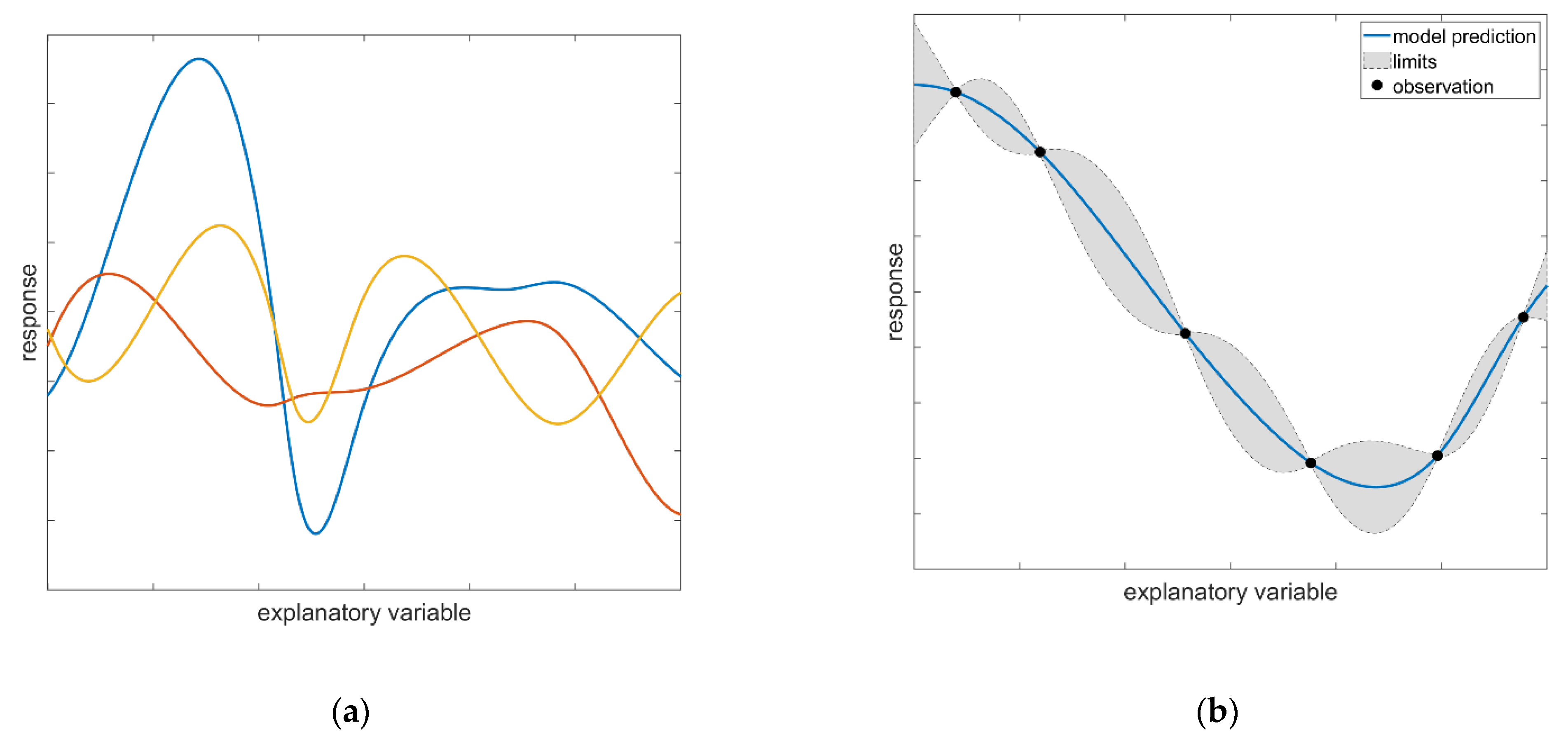
By incorporating the observation from the training data, functions which do not pass the data points (or do not closely pass in case of noisy data) are removed from the infinite set, in order to form the posterior distribution. As a result, the posterior uncertainty in the vicinity of the observations is reduced. This is also called conditioning of the Gaussian prior distribution on the observations. In Figure 2a three samples from the prior distribution are shown. The posterior distribution after observation of five data points is depicted in Figure 2b. The underlying (unknown) function is a polynomial of the third degree. Making a prediction using the Gaussian process ultimately amounts to drawing samples from its posterior distribution.
That being said, the predictive performance of Gaussian processes depends exclusively on the chosen kernel [24]. For prediction of the electric energy demand the Matérn covariance function with v = 3 / 2 given in Equation (7) was chosen. In contrast to other popular kernels, such as the infinitely differentiable squared exponential kernel displayed in Equation (8) (Gaussian function), its shape is rather rough. However, strong smoothness is argued to be unrealistic for modelling of physical processes [25].
k v = 3 / 2 ( r ) = ( 1 + 3 r l ) e x p ( 3 r l )
k S E ( r ) = e x p ( r 2 2 l 2 )
The performance of the models on the validation data is evaluated using the adjusted coefficient of determination ( R 2 ) , as well as the mean absolute error (MAE), standard deviation of the result (SD) and relative standard deviation (RSD). These values are calculated as shown in Equations (9)–(12). The relative standard deviation (coefficient of variation) is utilized in order to illustrate the extend of variability in relation to the average demand of electric energy [26]. The mean values of the measured and calculated electric energy demand is denoted as y ¯ and f ¯ , respectively. The coefficient of determination ranges from 0 to 1 and is often used as an indicator for the goodness of the fit, with 1 meaning the results perfectly match the measurements.
R 2 = 1 R S S T S S = 1   ( f i y i ) 2   ( y i y ¯ ) 2
M A E =   [ f i y i ] n
S D =   ( f i f ¯ ) 2 n
R S D = S D y ¯

2.2. Datasets of EAF Heats Used in This Study

For evaluation of the described models, process data of five electrical arc furnaces for industrial steel production was used. In total, the data sets contain material consumption and furnace operation data of roughly 21,000 heats. However, the investigated furnaces differ considerably regarding their capacity and material input, as well as the measurements taken during operation. The characteristics of the furnaces are summarized in Table 2. With an average tap weight of about 80 t EAF-A has a notably smaller capacity than the remaining furnaces. Likewise, the average tap-to-tap time of EAF-A is shorter. Furnace B, C and D have similar capacities and tap-to-tap times. The highest specific electrical energy demand is found for EAF-C. The different specific electric energy demand of the furnaces can in part be attributed to the differences in the charged ferrous material. For both EAF-B and EAF-C, the input material contains large quantities of DRI or HBI while the remaining furnaces use scrap of varying quality.
Not all documented heats can be used for evaluation of the electric energy demand. In the first step data, treatment is performed on each set. The overall goal is the removal of faulty or irregular data originating from erroneous data logging or irregular operation such as trial heats, aborted heats, or equipment malfunctions. Including these heats would otherwise have a negative impact on training of the models for regular heats, which are the main subject of the investigation. Table 2 shows the total amount and the percentage of excluded heats. In the following the applied decision rules for removal of data are described.
When crucial data like electric energy demand or tap weight are missing, the applied regression models cannot accurately predict the electrical energy demand, and therefore the heats in question must be excluded from consideration. In addition, heats are excluded if the measurements are unreasonable. This is, for example, the case if the tap weight exceeds the maximum capacity of the furnace, or the recorded tap-to-tap time is lower than the power on time of the heat. Significant outliers were also removed from the data sets. These include heats with an abnormal tap-to-tap time since they are likely to contain long power off times as a result of production delays by unscheduled events or regular maintenance stops. Likewise, heats are removed if the number of buckets differs from the rest of the batches. Finally, heats are removed if their ratio between charged ferrous material and tapped steel is below 0.75 or above 1.05, respectively. This is due to the mass of the hot heel not being measured for most of the furnaces. In keeping part of the molten steel inside the furnace after tapping, the melting rate of the subsequent heat can be increased. This results in lower thermal losses and a lower overall energy demand [27]. Moreover, in DC furnaces a hot heel is necessary for operation as it is covering the electrode in the bottom of the vessel and closes the circuit. However, when the furnace is completely emptied the amount of energy needed for initial melting of the hot heel is unaccounted for, while the energy demand of the next heat is higher compared to regular heats. In consequence, these heats, usually occurring before and after maintenance periods, are removed from consideration. In total, between 3% and 13% of the heats were removed. EAF-C, EAF-D and EAF-E show a notable larger percentage of the excluded data compared to EAF-A and EAF-B. This can mostly be attributed to unusually long heats, i.e., frequent production interruptions (270 for EAF-C and 160 for EAF-E) and missing measurements or recorded data. For EAF-D 775 out of 785 removed heats are missing the mass of charged material and about 270 heats from EAF-C are lacking temperature measurement from the molten steel.
Apart from the data quality and overall differences in the operation of the furnaces, the amount of data recorded during operation also differs significantly. Table 3 shows an overview of the available measurements. The electric energy demand, as well as the mass of charged ferrous material, coal and slag formers are measured for all furnaces. For the first three furnaces only a basic breakdown into scrap, DRI and alloying metals is given while EAF-D and EAF-E have a detailed record of the charged scrap grades. The exact chemical composition of the input materials is, however, unknown and is likely to differ between plants and even between heats. Furthermore, the mass of charged slag former in EAF-B and EAF-C is provided with an accuracy of 0.5 tons. This suggests that the stated mass is estimated or measured with limited accuracy only. Although this was the only obvious case it must be noted that all measurements are associated with a degree of uncertainty since no information on the methods and accuracy of the measurements was given.
During operation, the injected oxygen and carbon mass was measured along with the consumption of natural gas. EAF-B is the only furnace without operation of natural gas burners. Moreover, in the records from EAF-D and EAF-E, oxygen input is further separated into different applications within the furnace such as oxygen for burners, lances, or post-combustion. In the remaining data sets oxygen input is separated only for the purpose of post-combustion with all other flows combined into a single measurement. Power-on time as well as tap-to-tap time are measured for all furnaces, yet only EAF-A and EAF-E have a detailed breakdown of sub-process times such as charging, melting, and tapping provided. Energy losses can vary considerably throughout the different stages of the melting process. Therefore, by providing information on the length of the sub-processes the quality of the prediction can be improved. Furthermore, the weight and temperature of the tapped steel are available. Temperature measurement is carried out shortly before tapping in order to ensure the target temperature was reached. The temperature and mass of the tapped steel are directly related to the energy demand for melting. As stated before, the mass of the hot heel which remains inside the vessel after tapping is however only measured at two of the furnaces with the method and accuracy of the measurement unknown. Lastly, at EAF-D the composition of both steel and slag is analyzed after each heat, while EAF-E has steel composition measured in regular intervals for 98 heats in total. As can be seen from the overview of furnace characteristics in Table 2 and measurements in Table 3 a single regression model cannot be applied for all furnace without the need to drastically reduce the data sets in order to form a common denominator. Even in doing so, the measurements are performed with different precision and in the case of scrap grades and slag formers classification is not necessarily uniform. In consequence the furnaces must be considered separately, while the general design of the investigated models is maintained.
For each furnace, heats are divided into a training and validation set. The training set contains 70% of the data and is drawn at random. Subsequent validation is performed on the remaining 30% of heats. All applied models are trained on the same data set. However, since selection of the training data influences the model accuracy, training and validation are performed on 5 separate training samples and the median results of the regressions are discussed. Beyond that, process data can be divided into two groups: measurements available before and only after the heat is finished. In the literature the entire dataset is often used for modeling of the electric energy demand [11,17,20,28]. While those models yield better results in terms of accuracy, they cannot be applied to predict the energy demand of a future heat. Subsequently, the investigated regression models will be used on the entire and limited dataset and the results of both approaches will be compared.

3. Results

At first the results of the Köhle formula were calculated for each EAF. In place of the furnace-specific parameter N V , a bias was added to the results, such that the average deviation for each furnace assumes the value of 0. The MAE, SD, and RSD for prediction of the electric energy demand of single heats is presented in Table 4. The results show that the accuracy of prediction significantly differs between the furnaces, with the best result obtained for EAF-B. This is likely due to EAF-B only having DRI and hot metal charged. Both input materials are represented in the Köhle formula while different scrap grades are not considered, resulting in a large deviation of the calculated energy demand.
Subsequently, the previously described regression models were applied to the process data of the five EAFs. After parameter optimization on the training data was finished, the regression models were used to estimate the electric energy demand of the heats within the test set. The median results of the regression models on the entire dataset are summarized in Table 5. For the sake of comparability, the mean absolute error and standard deviation are calculated using the specific electric energy demand rather than the absolute electric energy demand. The coefficient of determination is calculated on the absolute electric energy demand per heat. It can be seen from the table that the Gaussian process regression shows the best overall accuracy with regards to the mean absolute and standard deviation as well as the coefficient of determination, ranging from 0.651 to 0.941 for the investigated furnaces. That being said, by applying a multiple linear regression the quality of prediction can still be significantly improved compared to the results of the Köhle formula on single heats.
By utilizing a Gaussian process regression for EAF-B and EAF-C the mean absolute deviation, as well as the relative standard deviation of the results can be decreased by approximately 30% when compared to the results of the linear regression. In contrast with the remaining furnaces, the benefit of applying nonlinear models is notably lower, with EAF-A and EAF-D hardly showing any differences between the investigated models. A possible reason might be the use of DRI in both EAF-B and EAF-C instead of the various scrap grades. Although a larger amount of energy is required for the melting of DRI [12], the variance in chemical composition of the material is lower than that of the scrap mix. The charged scrap can have various contaminants which affect the process and energy requirement for melting. At the same time, at the remaining furnaces the number of heats including individual scrap grades is significantly lower when compared to the number of heats containing DRI at EAF-B and EAF-C. The smaller effective sample size could have a negative impact on training of the ANN in particular. In Figure 3 the electric energy demand of EAF-C is displayed in relation to the percentage of charged DRI and the number of baskets. As can be seen in the diagram, a large number of samples is available for each category. By applying an ANN or GPR, the nonlinear relationship between these process parameters can be modelled and its large-scale effect on the electric energy demand is estimated more accurately than by using a linear regression on the raw data. For the remaining furnaces, the smaller sample size for the input of individual scrap grades and higher variance within grades results in an equal level of accuracy across the model types, even when considering possible nonlinear interaction.
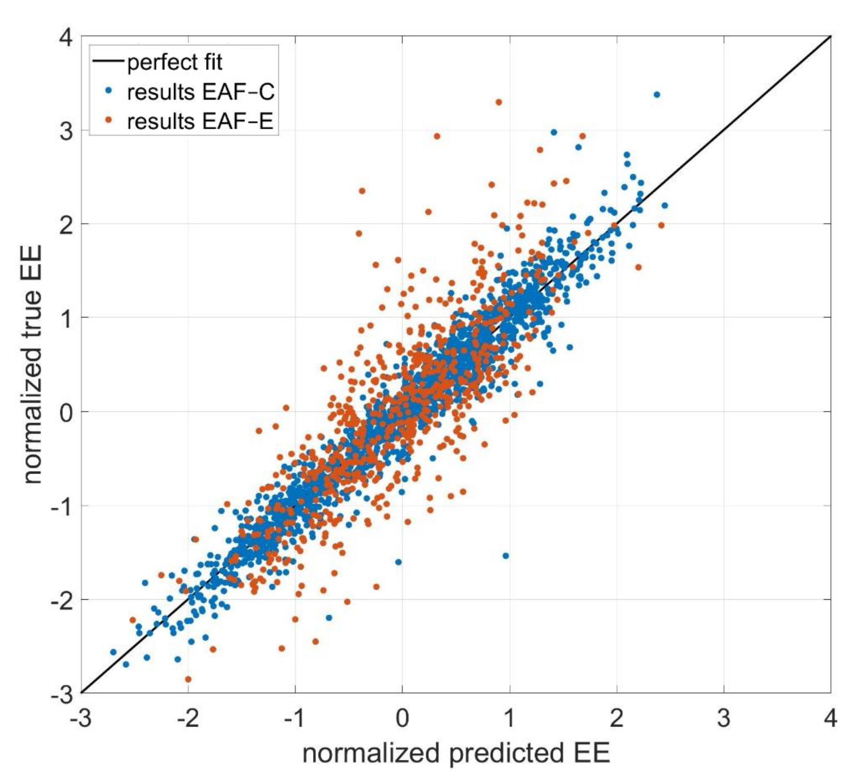
Furthermore, although EAF-E exhibits the smallest coefficient of determination (implying a larger deviation between the model results and measurements) its mean absolute error and standard deviation are in fact the smallest among the investigated furnaces. On average the regression models deviate from the true electric energy demand by 721 kWh/heat for EAF-E and 1789 kWh/heat for EAF-C, i.e., 5.9 kWh/t for EAF-E and 12.6 kWh/t for EAF-C. The difference in average tap weight displayed in Table 2 cannot explain the large deviation. This is also shown in by the relative standard deviations for both furnaces. As is stated in Equation (7), the coefficient of determination represents the ratio between the deviation of the calculated electric energy demand from the average measured demand and the measured deviation from its mean value. It is often interpreted as the proportion of energy demand which is explained by the regression model [29]. As depicted in Figure 3 the electric energy demand of EAF-C spans between roughly 40 MWh and 100 MWh per heat in contrast to the much narrower production parameters of EAF-E. As a result, the calculated ratio is smaller for EAF-C, although the electric energy demand is more accurately described for EAF-E.
In consequence, when discussing the accuracy of regression models for multiple furnaces, the coefficient of determination on its own is not suited for evaluation. In this context, the values for R 2 given in the literature must also be examined critically as the investigated furnaces most likely differ as well. The same applies to depictions of normalized results. In this regard, in Figure 4 the normalized estimated energy demand of EAF-C and EAF-E are compared. For EAF-E the model appears to predict the measurement more accurately. However, in terms of absolute values, the residuals for EAF-C are on average about twice that to the results of EAF-E as stated in Table 5.
Another problem arises from measurements being unavailable until the heat is finished. Naturally, this involves for example the tap weight and steel temperature as well as the consumption of natural gas and oxygen. As mentioned before, training of the regression models is therefore repeated for a reduced data set, containing only the mass of material charged at the start of each heat. The aim is to evaluate the applicability of the regression models for prediction of the electric energy demand of future heats. In Table 6 the results of the applied regression algorithms on the limited data set are shown. In comparison to the previous results in Table 5 a significant reduction in the quality of the model results can be observed. Application of the GPR still yields the best overall results; nevertheless, the mean absolute error calculated on the validation data is increased by up to 10 kWh/t. The standard deviation rises on an equal scale. Similar to the previous case, the largest difference between the models can be found for EAF-B and EAF-C. This suggests that the difference in charged input materials is indeed responsible for the inconsistent performance of the applied nonlinear regressions. On the other hand, the drastically reduced prediction quality illustrates the information lost by removing the a-posteriori measurements. Considering arc furnaces are usually operated on distinct power levels, power-on time of the arc, for example, is closely correlated to the electric energy demand. Including the power-on time therefore naturally increases the accuracy of the model. However, process times might also be an indicator for the quality of the input material. Likewise, injection of coal and consumption of natural gas are directly reducing the demand of electric energy by supplying chemical energy. Yet excessive consumption of natural gas and coal can also indicate poor operation, resulting in long tap-to-tap as well as power-on time and ultimately a high electric energy demand. When predicting the energy demand of future heats, these in-process measurements are, however, unavailable. The difference in the quality of results is particularly high when a large number of different scrap types is used, as can be seen from the results of EAF-A and EAF-D in Table 5 and Table 6. Another reason for the differences in the results is the use of natural gas, carbon, oxygen, and other additives, which can vary considerably between single heats, corresponding to irregularities in the operation of the furnace or contaminants within the ferrous material.
On a side note, the correlation between the consumption of coal, natural gas, and oxygen with the demand of electric energy in the EAF can result in positive parameter values for these explanatory variables. Interpretation of the parameter values would imply an increase in energy demand through the use of coal for example. However, a regression model cannot provide direct information on causality, which has to be kept in mind when interpreting the results [29]
In an attempt to utilize all available information, training of model parameter was carried out using the entire data set, while applying only the limited data for validation of the results on the test data. Missing values, such as consumption of natural gas and oxygen, were replaced by mean values of previous heats. However, this approach yielded very similar results as displayed in Table 6. In this regard, investigation of the consumption of natural gas, carbon, oxygen, and other additives in relationship to the material input and produced steel grade is required. By further classification of the heats, the variation of process parameters within the subsets can possibly be limited and prediction accuracy on future heats can be improved. In this context, an analysis of the quantity of contaminants within single scrap types would be beneficial.

4. Discussion

Within this study, the applicability of three different approaches for regression were examined in order to estimate the demand of electric energy in the operation of an electric arc furnace. To this end, the examined methods were tested on process data containing over 21,000 heats originating from five industrial-size EAFs.
Application of Gaussian process regression yielded the best overall results in terms of prediction accuracy. In some cases, the mean error, as well as the standard deviation, could be reduced by up to 30% compared to the linear regression. However, large differences were found across the investigated furnaces. The quality of the measured data was identified as one of the main reasons for the inconsistent behavior. This includes the categorization of charged scrap grades and slag formers. In general, application of a wide range of materials resulted in a lower accuracy of the implemented models as opposed to the predominant use of single grades with limited variance such as DRI. Even in utilizing non-linear methods, during training the models are unable to appropriately tune the weights or parameters due to, for example, various contaminants affecting the chemical composition. In consequence, the benefit of applying nonlinear models over linear regression is heavily dependent on the process parameters and measurement quality. In this regard, the crucial role of in-process measurements on the model precision was highlighted. However, when predicting the energy demand of future heats, this information cannot be used. Careful classification of the charged scrap types and slag formers is therefore particularly important in order to increase the model accuracy, and including further information on the properties of the charged material is recommended, if possible.
Lastly, by comparison of the achieved results, it was shown that the often-reported coefficient of determination is not sufficient for evaluation of a model’s predictive quality since the metric is heavily influenced by the observed variation in the target values. The same argument was given for evaluation of normalized results.

Author Contributions

Conceptualization, A.R.; methodology, A.R.; software, A.R.; validation, A.R.; formal analysis, A.R.; investigation, A.R.; resources, A.R., T.E., H.P.; data curation, A.R.; writing—original draft preparation, A.R.; writing—review and editing, A.R., T.H., T.E. and M.K.; visualization, A.R.; supervision, T.E., H.P.; project administration, T.E., H.P. All authors have read and agreed to the published version of the manuscript.

Funding

This research received no external funding.

Institutional Review Board Statement

Not applicable.

Informed Consent Statement

Not applicable.

Data Availability Statement

Data sharing not applicable.

Conflicts of Interest

The authors declare no conflict of interest.

References

  1. World Steel Association. Steel Statistical Yearbook 2019: Concise Version; World Steel Association: Brussels, Belgium, 2019. [Google Scholar]
  2. Wirtschaftsvereinigung Stahl. Statistisches Jahrbuch der Stahlindustrie: 2020|2021; Wirtschaftsvereinigung Stahl: Berlin, Germany, 2021. [Google Scholar]
  3. European Commission. Climate Strategies & Targets. Available online: https://ec.europa.eu/clima/policies/strategies_en (accessed on 29 June 2021).
  4. Carlsson, L.S.; Samuelsson, P.B.; Jönsson, P.G. Predicting the Electrical Energy Consumption of Electric Arc Furnaces Using Statistical Modeling. Metals 2019, 9, 959. [Google Scholar] [CrossRef] [Green Version]
  5. Hay, T.; Visuri, V.-V.; Aula, M.; Echterhof, T. A Review of Mathematical Process Models for the Electric Arc Furnace Process. Steel Res. Int. 2021, 92, 2000395. [Google Scholar] [CrossRef]
  6. Bekker, J.G.; Craig, I.K.; Pistorius, P. Modeling and Simulation of an Electric Arc Furnace Process. ISIJ Int. 1999, 39, 23–32. [Google Scholar] [CrossRef] [Green Version]
  7. Logar, V.; Dovžan, D.; Škrjanc, I. Modeling and Validation of an Electric Arc Furnace: Part 1, Heat and Mass Transfer. ISIJ Int. 2012, 52, 402–412. [Google Scholar] [CrossRef] [Green Version]
  8. Logar, V.; Dovzan, D.; Škrjanc, I. Modeling and Validation of an Electric Arc Furnace: Part 2, Thermo-chemistry. ISIJ Int. 2012, 52, 413–423. [Google Scholar] [CrossRef] [Green Version]
  9. MacRosty, R.D.M.; Swartz, C.L.E. Dynamic Modeling of an Industrial Electric Arc Furnace. Ind. Eng. Chem. Res. 2005, 44, 8067–8083. [Google Scholar] [CrossRef]
  10. Cameron, I.T.; Hango, K. Process Modelling and Model Analysis; Academic Press: London, UK, 2001; ISBN 978-0121569310. [Google Scholar]
  11. Kleimt, B.; Köhle, S.; Kühn, R.; Zisser, S. Application of models for electrical energy consumption to improve EAF operation and dynamic control. In Proceedings of the 8th European Electric Steelmaking Conference, proceedings. European Electric Steelmaking Conference, Birmingham, UK, 9–12 May 2005. [Google Scholar]
  12. Pfeifer, H.; Kirschen, M.; Simoes, J.-P. Thermodynamic analysis of electrical energy demand. In Proceedings of the 7th European Electric Steelmaking Conference, Venice, Italy, 26–29 May 2002; pp. 1.413–1.428, ISBN 88-85298-44-3. [Google Scholar]
  13. Kirschen, M.; Zettl, K.-M.; Echterhof, T.; Pfeifer, H.; Models for EAF Energy Efficiency. Steel Times International [Online], 6 April 2017. Available online: https://www.steeltimesint.com/features/models-for-eaf-energy-efficiency (accessed on 25 July 2021).
  14. Kleimt, B.; Pierre, R.; Kordel, T.; Rekersdrees, T.; Schlinge, L.; Hellermann, O.; Elsabagh, S.; Haverkamp, V.; Gogolin, S. Adaptive EAF Online Control Based on Innovative Sensors and Comprehensive Models for Improved Yield and Energy Efficiency; European Commission: Brussels, Belgium, 2019; ISBN 978-92-79-98359-7. [Google Scholar]
  15. Malfa, E.; Nyssen, P.; Filippini, E.; Dettmer, B.; Unamuno, I.; Gustafsson, A.; Sandberg, E.; Kleimt, B. Cost and Energy Effective Management of EAF with Flexible Charge Material Mix. BHM Berg-und Hüttenmännische Mon. 2013, 158, 3–12. [Google Scholar] [CrossRef]
  16. Conejo, A.N.; Cárdenas, J. Energy Consumption in the EAF with 100% DRI. In Proceedings of the AISTech 2006 Conference, Cleveland, OH, USA, 1–4 May 2006; pp. 529–535. [Google Scholar]
  17. Carlsson, L.S.; Samuelsson, P.B.; Jönsson, P.G. Using Statistical Modeling to Predict the Electrical Energy Consumption of an Electric Arc Furnace Producing Stainless Steel. Metals 2019, 10, 36. [Google Scholar] [CrossRef] [Green Version]
  18. Gajic, D.; Gajic, I.S.; Savic, I.; Georgieva, O.; Di Gennaro, S. Modelling of electrical energy consumption in an electric arc furnace using artificial neural networks. Energy 2016, 108, 132–139. [Google Scholar] [CrossRef]
  19. Baumert, J.-C.; Engel, R.; Weiler, C. Dynamic modelling of the electric arc furnace process using artificial neural networks. Revue de Métallurgie 2002, 99, 839–849. [Google Scholar] [CrossRef]
  20. Chen, C.; Liu, Y.; Kumar, M.; Qin, J. Energy Consumption Modelling Using Deep Learning Technique—A Case Study of EAF. Procedia CIRP 2018, 72, 1063–1068. [Google Scholar] [CrossRef]
  21. Bowman, B.; Krüger, K. Arc Furnace Physics; Verlag Stahleisen: Düsseldorf, Germany, 2009; ISBN 9783514007680. [Google Scholar]
  22. Goodfellow, I.; Bengio, Y.; Courville, A. Deep Learning; The MIT Press: Cambridge, MA, USA, 2016; ISBN 0262035618. [Google Scholar]
  23. Rasmussen, C.E.; Williams, C.K.I. Gaussian Processes for Machine Learning, 1st ed.; The MIT Press: Cambridge, MA, USA, 2016; pp. 33–77. [Google Scholar]
  24. Murphy, K.P. Machine Learning: A Probabilistic Perspective; MIT Press: Cambridge, MA, USA, 2013; ISBN 978-0262018029. [Google Scholar]
  25. Stein, M.L. Interpolation of Spatial Data: Some Theory for Kriging, 1st ed.; Springer: New York, NY, USA, 1999; ISBN 978-0-387-98629-6. [Google Scholar]
  26. Hartung, J.; Elpelt, B.; Klösener, K.-H. Statistik: Lehrund Handbuch der Angewandten Statistik; Oldenbourg Wissenschaftsverlag: Munich, Germany, 2012; ISBN 978-3-486-71054-0. [Google Scholar]
  27. Toulouevski, Y.; Zinurov, I. Innovation in Electric Arc Furnaces: Scientific Basis for Selection; Springer: Berlin, Germany, 2010; ISBN 978-3-642-03800-6. [Google Scholar]
  28. Kovačič, M.; Stopar, K.; Vertnik, R.; Šarler, B. Comprehensive Electric Arc Furnace Electric Energy Consumption Modeling: A Pilot Study. Energies 2019, 12, 2142. [Google Scholar] [CrossRef] [Green Version]
  29. Wooldridge, J.M. Introductory Econometrics: A Modern Approach, 5th ed.; South Western Educ Pub: Mason, OH, USA, 2012; ISBN 978-1-111-53104-1. [Google Scholar]
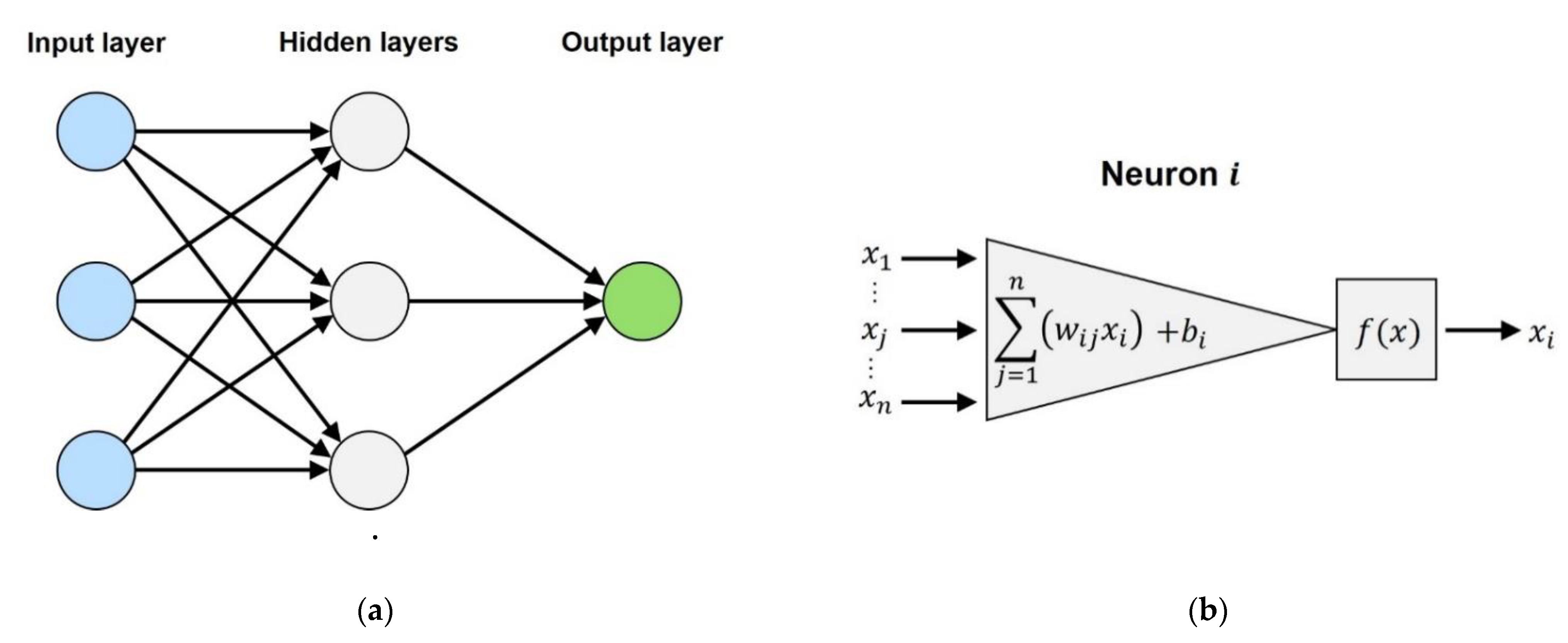
Figure 1. (a) structure of feedforward neural net featuring a single hidden layer; (b) calculation of the output of a neuron and transfer function.
Metals 11 01348 g001
Figure 2. (a) three samples of the prior distribution specified by the mean and covariance function; (b) posterior distribution after observation of six data points.
Metals 11 01348 g002
Figure 3. (a) Percentage of DRI charged in EAF-C with varying number of baskets; (b) Comparison of the estimated electric energy demand for EAF-C and EAF-E.
Metals 11 01348 g003
Figure 4. Comparison of normalized estimated electric energy demand of EAF-C and EAF-E.
Metals 11 01348 g004
Table 1. Parameters of the Köhle formula.
ParameterNameUnitParameterNameUnit
G A Tap weightt t s Power-on timemin
G E Weight of ferrous materialt t N Power-off timemin
G D R I / H B I Weight of DRIt M G Specific burner gas m 3 t
G S H R Weight of HBIt M L Specific lance oxygen m 3 t
G H M Weight of hot metalt M N Specific post-combustion oxygen m 3 t
G Z Weight of slag formerst N V Furnace specific factor-
T A Tapping temperature°C W V Energy losses k W h t
Table 2. Specification and key performance indicators of the investigated electric arc furnaces.
FurnaceEAF-AEAF-BEAF-CEAF-DEAF-E
Average tap weight [t]81153142142123
Average tap-to-tap time [min]4562696157
Average specific electric energy demand [kWh/t]325467535422345
Ferrous MaterialScrapDRIDRI/Scrap MixScrapScrap
Number of overall heats52201046613980882341
Number of excluded heats15032791785163
Percentage of removed heats2.93.112.89.77.0
Table 3. Overview of the available measurements at the investigated EAFs.
FurnaceEAF-AEAF-BEAF-CEAF-DEAF-E
Electric energy demand [kWh]xxxxx
Mass of charged scrap grades [t]xxxx1x1
Mass of slag formers [t]xxxx1x1
Charged or injected Coal [t]xxxxx
Bath height [m]----x
Oxygen consumption [m3](x)(x)(x)xx
Natural gas consumption [m3]x2-xxx
Power-on time [min]xxxxx
Tap-to-tap time [min]xxxxx
Sub-process times [min]x---x
Tap weight [t]xxxxx
Melt temperature [°C]xxxxx
Mass of hot heel [t]-x--x
Steel composition [kg/kg]---x(x)
Slag composition [kg/kg]---(x)-
(x): only limited information available; x1: detailed record of scrap grades; x2: chemical heat input provided in kWh.
Table 4. Results of the Köhle formula on the investigated furnaces.
Model PerformanceEAF-AEAF-BEAF-CEAF-DEAF-E
MAE [kWh/t]25.114.831.621.140.0
SD [kWh/t]36.019.041.627.353.1
RSD [%]11.14.17.86.515.4
Table 5. Median result of the applied regression algorithms on the entire data set for validation.
FurnaceModel PerformanceLinear RegressionANNGPR
EAF-A R 2 0.8420.8470.859
MAE [kWh/t]7.97.67.1
SD [kWh/t]11.210.510.6
RSD [%]3.43.23.3
EAF-B R 2 0.8990.8710.943
MAE [kWh/t]11.712.78.3
SD [kWh/t]15.416.411.1
RSD [%]3.33.52.4
EAF-C R 2 0.8810.9230.941
MAE [kWh/t]14.912.310.3
SD [kWh/t]20.816.414.4
RSD [%]3.93.12.7
EAF-D R 2 0.7540.7550.769
MAE [kWh/t]9.99.99.6
SD [kWh/t]12.812.812.4
RSD [%]3.03.02.9
EAF-E R 2 0.5190.5870.651
MAE [kWh/t]6.35.85.3
SD [kWh/t]8.47.87.2
RSD [%]2.42.32.1
Table 6. Median results for regression on the data available before finishing of the heat.
FurnaceModel PerformanceLinear RegressionANNGPR
EAF-A R 2 0.1850.1830.227
MAE [kWh/t]17.417.417
SD [kWh/t]24.424.523.7
RSD [%]7.57.57.3
EAF-B R 2 0.710.7480.821
MAE [kWh/t]20.317.013.4
SD [kWh/t]24.723.019.4
RSD [%]5.34.94.2
EAF-C R 2 0.7420.7550.853
MAE [kWh/t]24.321.917.0
SD [kWh/t]30.629.823.1
RSD [%]5.75.64.3
EAF-D R 2 0.2440.2420.228
MAE [kWh/t]17.317.317.2
SD [kWh/t]22.522.522.7
RSD [%]5.35.35.4
EAF-E R 2 0.2450.2990.360
MAE [kWh/t]8.07.57.3
SD [kWh/t]10.510.19.7
RSD [%]3.02.92.8
Publisher’s Note: MDPI stays neutral with regard to jurisdictional claims in published maps and institutional affiliations.