Mathematical Methodology and Metallurgical Application of Turbulence Modelling: A Review

Abstract

This paper focusses on three main numerical methods, i.e., the Reynolds-Averaged Navier-Stokes (RANS), Large Eddy Simulation (LES), and Direct Numerical Simulation (DNS) methods. The formulation and variation of different RANS methods are evaluated. The advantage and disadvantage of RANS models to characterize turbulent flows are discussed. The progress of LES with different subgrid scale models is presented. Special attention is paid to the inflow boundary condition for LES modelling. Application and limitation of the DNS model are described. Different experimental techniques for model validation are given. The consistency between physical experimentation/modelling and industrial cases is discussed. An emphasis is placed on the model validation through physical experimentation. Subsequently, the application of a turbulence model for three specific flow problems commonly encountered in metallurgical process, i.e., bubble-induced turbulence, supersonic jet transport, and electromagnetic suppression of turbulence, is discussed. Some future perspectives for the simulation of turbulent flow are formulated.

1. Introduction

Since turbulence plays a significant role in flow transport phenomena, considerable efforts have been devoted to understanding flow turbulence in both engineering and academic communities [1,2,3,4]. Nevertheless, turbulence is still not fully understood due to its complexities in nature, e.g., instantaneous and intermittency characteristics, strong nonlinearity, and a wide range of temporal and spatial scales [4,5].

Turbulent flow can be numerically resolved with different levels of accuracy. Many numerical approaches for solving turbulence have been proposed, such as the Reynolds-Averaged Navier–Stokes (RANS) [6,7,8,9,10,11], the Large Eddy Simulation (LES) [12,13,14], and Direct Numerical Simulation (DNS) approaches [15]. Among these numerical methods, the RANS approach, specifically the Eddy Viscosity Model (EVM), is widely used for calculating turbulent flows thanks to its relatively high accuracy in predicting the mean flow features and its more limited computational demands. However, this approach suffers from several weaknesses, e.g., compromised accuracy and uncertainties due to assumptions in the model construction and insufficient incorporation of the fluid physics. In the LES approach, the whole eddy range is separated into two parts, namely, the large-scale eddy and subgrid-scale (SGS) eddy. The former can be directly resolved, while the latter is computed using the SGS model. As the computing power rapidly increases, this approach is extensively used to study turbulence physics and to resolve low-to-medium Reynolds number flows. In order to obtain meaningful results, additional attention is paid to inflow boundary conditions and mesh density for LES modelling. Compared to the RANS and LES, the DNS approach is the most accurate numerical method because it directly resolves all the turbulent eddies without using any models. However, DNS requires extensive computational demands to solve turbulent engineering flows, which is difficult to be satisfied by the current computing power. In addition, the large amount of data generated by DNS should be carefully analyzed.

Due to the uncertainties of the RANS method, many model variants have been proposed to solve specific turbulent flows [6,7,8,9,10], which can easily confuse the users of Computational Fluids Dynamics (CFD) codes to choose an appropriate one for their own cases. A comprehensive and well-organized description of the model formulation and development is very helpful in judging the applicability of different models, although there are some works with respect to model description [1,3]. Apart from SGS models of the LES method, the inflow boundary condition is an indispensable part of the simulation. Considering a diversity of methods generating inflow information [16,17], an elaborate analysis and discussion on the methods is necessary and conducive for the LES model user. In order to clearly understand the potential of the DNS method, the capabilities and current limitations of DNS method need to be clarified. In addition to the numerical solutions for turbulent flows, model validation is needed to warrant the accuracy of the simulation. Depending on different studies, different physical experimentations assisted with measuring techniques are performed to validate the numerical model. There are a number of studies focusing on the fundamentals of different measuring techniques, data interpretation, and applications of the techniques [18,19]. However, the consistency between physical experimentation/modelling and industrial applications needs to be discussed. The limitations and development of the measuring techniques are critical for obtaining reliable data and should be reviewed.

In this work, we review the formulation and development of three main numerical approaches (i.e., the RANS, LES, and DNS) for turbulence modelling. The advantages and disadvantages of the approaches are systematically discussed. Different methods of the inflow boundary condition are described for LES modelling. For the purpose of validating numerical models, different physical experimentation methods are presented. The consistency between the physical modelling and industrial applications is discussed. Limitations and progress of the experimental validation techniques are shown. Three turbulence-related flow problems commonly encountered in metallurgical fields (i.e., bubble-induced turbulence (BIT), supersonic jet transport, and electromagnetic damping of turbulence) are discussed to demonstrate how to customize a conventional turbulence model for solving a specific flow problem. Finally, perspectives for modelling turbulent flows are proposed. With this review, we intend to help the current and potential CFD users to understand the modelling techniques for turbulence flows better and to expand the insight into the physics of turbulence.

2. Turbulence Simulation Approaches

2.1. RANS

In the RANS approach, instantaneous solution variables in the governing equations are decomposed into the mean and fluctuating components, as expressed in Equation (1).

$$f=\overline{f}+f^{\prime }$$

(1)

Substituting this variable expression into the instantaneous continuity and Navier-Stokes (N-S) equations yields the ensemble- or time-averaged forms for single-phase Newtonian flow, as shown in Equations (2) and (3). Henceforth, repeated-suffix summation convention is used in the formulae.

$$\frac{\partial \rho }{\partial t}+\frac{\partial }{\partial x_i}\left(\rho {\overline{u}}_i\right)=0$$

(2)

$$\frac{\partial }{\partial t}\left(\rho {\overline{u}}_i\right)+\frac{\partial }{\partial x_j}\left(\rho {\overline{u}}_i{\overline{u}}_j\right)=-\frac{\partial \overline{p}}{\partial x_i}+\frac{\partial }{\partial x_j}\left(\mu \frac{\partial {\overline{u}}_i}{\partial x_j}-\rho \overline{u_i^{\prime }{u}_j^{\prime }}\right)$$

(3)

The fluctuating quantities are included in the Reynolds stress tensor ($-\rho \overline{u_i^{\prime }{u}_j^{\prime }}$) with six components. In order to close the equation set, the Reynolds stress tensor needs to be appropriately solved. One of the solutions for this closure problem employs the Boussinesq assumption [20], which relates the Reynolds stresses to the mean velocity gradients. The advantage of the Boussinesq assumption is the relatively low computational cost due to its simplicity. This works well for the engineering flows, which are dominated by only one turbulent shear stress such as the jet flow, wall boundary layer flow, and mixing layers flow. However, this approach is insensitive to the streamline curvature, rotation and body forces, and it exhibits a poor performance in the flows with a strong anisotropy or stress transport effect [21,22]. It also has difficulty in predicting transitional flows.

It is worth noting that the turbulent viscosity used in solving the Reynolds stress terms is a function of the space and flow features, rather than a physical parameter such as the fluid viscosity, which is dependent on the molecular structure of the fluid. Obviously, the turbulent viscosity needs to be solved before computing the Reynolds stress terms. In this paper, two-equation models, which include two additional transport equations, are reviewed. Usually the turbulence kinetic energy (k) is adopted as one equation and the turbulent kinetic energy dissipation rate (ε) or the specific dissipation rate (ω) as another one. The modified versions of the ε/ω model will also be presented here. Due to length restrictions, the zero- and one-equation models are not included in the article, but they may be found elsewhere [23,24,25].

2.1.1. The k-ε Model

The standard k-ε (SKE) model was originally proposed by Launder and Spalding [6]. The model has been widely applied for resolving turbulent flows without a severe pressure gradient or strong swirling effect (e.g., plane jet, mixing layer, and boundary layer flows) because of its relatively high robustness, low computational cost, and reasonable accuracy. Equations (4) and (5) show the general form of k and ε. By solving these two transport equations, the turbulent viscosity can be calculated as expressed in Equation (6).

$$\frac{\partial }{\partial t}\left(\rho k\right)+\frac{\partial }{\partial x_i}\left(\rho k{\overline{u}}_i\right)=\frac{\partial }{\partial x_j}\left[\left(\mu +\frac{{\mu }_t}{{\sigma }_k}\right)\frac{\partial k}{\partial x_j}\right]-\rho \overline{u_i^{\prime }{u}_j^{\prime }}\frac{\partial {\overline{u}}_i}{\partial x_j}-\rho \epsilon +S_k$$

(4)

$$\frac{\partial }{\partial t}\left(\rho \epsilon \right)+\frac{\partial }{\partial x_i}\left(\rho \epsilon {\overline{u}}_i\right)=\frac{\partial }{\partial x_j}\left[\left(\mu +\frac{{\mu }_t}{{\sigma }_{\epsilon }}\right)\frac{\partial \epsilon }{\partial x_j}\right]-C_{1\epsilon }\frac{\epsilon }{k}\rho \overline{u_i^{\prime }{u}_j^{\prime }}\frac{\partial {\overline{u}}_i}{\partial x_j}-C_{2\epsilon }\rho \frac{{\epsilon }^2}{k}+S_{\epsilon }$$

(5)

$${\mu }_t=C_{\mu }\rho \frac{k^2}{\epsilon }$$

(6)

The terms from left to right in Equations (6) and (7) are the respective local time derivative, convection, diffusion, production, sink, and source terms. The SKE model is derived from a fully turbulent flow with high Reynolds numbers. The viscous effect is ignored in the model. However, this cannot be applied in the vicinity of the wall, where the viscous force dominates the flow characteristics. In order to deal with this problem, either a wall function is adopted with the SKE model, or a low Reynolds number model is used. The former confuses the users’ judgement whether the weakness of this method lies in the basic SKE model itself or in the wall function. The latter requires additional functions to modify the standard transport equations. With respect to the low Reynolds number models [26,27,28,29,30,31,32], an example proposed by Lam and Bremhorst (LB model) [31] is presented in Equations (7) and (8).

$$\frac{\partial }{\partial t}\left(\rho k\right)+\frac{\partial }{\partial x_i}\left(\rho k{\overline{u}}_i\right)=\frac{\partial }{\partial x_j}\left[\left(\mu +\frac{{\mu }_t}{{\sigma }_k}\right)\frac{\partial k}{\partial x_j}\right]+{\mu }_t\left(\frac{\partial {\overline{u}}_i}{\partial x_j}+\frac{\partial {\overline{u}}_j}{\partial x_i}\right)\frac{\partial {\overline{u}}_i}{\partial x_j}-\rho \epsilon$$

(7)

$$\frac{\partial }{\partial t}\left(\rho \epsilon \right)+\frac{\partial }{\partial x_i}\left(\rho \epsilon {\overline{u}}_i\right)=\frac{\partial }{\partial x_j}\left[\left(\mu +\frac{{\mu }_t}{{\sigma }_{\epsilon }}\right)\frac{\partial \epsilon }{\partial x_j}\right]+C_{1\epsilon }{f}_1\frac{\epsilon }{k}{\mu }_t\left(\frac{\partial {\overline{u}}_i}{\partial x_j}+\frac{\partial {\overline{u}}_j}{\partial x_i}\right)\frac{\partial {\overline{u}}_i}{\partial x_j}-C_{2\epsilon }{f}_2\rho \frac{{\epsilon }^2}{k}$$

(8)

where:

$${\mu }_t=C_{\mu }{f}_{\mu }\rho \frac{k^2}{\epsilon }$$

(9)

Compared with the SKE model, different formulations of functions $f_1$, $f_2$ and $f_{\mu }$ are developed in the LB model to describe the near-wall behavior better. It has been confirmed that the function $f_{\mu }$ has a predominant influence on the model performance, and functions $f_1$, $f_2$ play a secondary role in the performance [11].

There are also other modified versions of the SKE model, amongst which the widely used Renormalization Group (RNG) k-ε model [7] and the Realizable k-ε (RKE) model [8] are introduced in the following section. The main differences between the RNG k-ε model and the SKE model are the modifications of the turbulent viscosity and ε sink term. A differential equation is analytically derived for effective viscosity ${\mu }_{eff}$ to account for the low Reynolds number effect. This feature can improve the predictive ability of the RNG k-ε model for low Reynolds number flows or near-wall flows. Additionally, a new ε destruction term is used to account for the rapid strain by modifying the constant of this term. The RKE model is modified mainly with regard to the turbulent viscosity and the ε equation. By defining a variable $C_{\mu }$ [8,33,34] instead of a constant value in turbulent viscosity formulation, the RKE model satisfies the realizability constraints, i.e., positive values for the normal stresses and the Schwartz inequality for the shear stresses. In order to increase the robustness of the model, a new ε equation is employed based on a dynamic equation for fluctuating vorticity. The new ε equation describes turbulent vortex stretching and turbulent dissipation more appropriately compared to the ε equation in the SKE model. With the modified ε equation, the well-known round-jet anomaly that is a poor prediction of the spreading rate of round/axisymmetric jet may be solved [8].

2.1.2. The k-ω Model

The k-ω model is widely used for turbulence modelling [35]. Different versions of this model have been developed in the last decades [9,10,36,37,38,39,40]. In this paper, the most well-known k-ω model proposed by Wilcox [9] is reviewed. The transport equations of this model are presented in Equations (10) and (11), where the calculation of β₁ refers to the work of Wilcox [9].

$$\frac{\partial }{\partial t}\left(\rho k\right)+\frac{\partial }{\partial x_i}\left(\rho k{\overline{u}}_i\right)=\frac{\partial }{\partial x_j}\left[\left(\mu +\frac{{\mu }_t}{{\sigma }_k}\right)\frac{\partial k}{\partial x_j}\right]-\rho \overline{u_i^{\prime }{u}_j^{\prime }}\frac{\partial {\overline{u}}_i}{\partial x_j}-\rho {\beta }^{\ast }k\omega +S_k$$

(10)

$$\frac{\partial }{\partial t}\left(\rho \omega \right)+\frac{\partial }{\partial x_i}\left(\rho \omega {\overline{u}}_i\right)=\frac{\partial }{\partial x_j}\left[\left(\mu +\frac{{\mu }_t}{{\sigma }_{\omega }}\right)\frac{\partial \omega }{\partial x_j}\right]-\alpha \frac{\omega }{k}\rho \overline{u_i^{\prime }{u}_j^{\prime }}\frac{\partial {\overline{u}}_i}{\partial x_j}-\rho {\beta }_1{\omega }^2+S_{\omega }$$

(11)

Unlike the k-ε model, the k-ω model can be integrated through the viscous sublayer without any damping function to account for the low Reynolds number effect with high numerical stability. Therefore, it is well applied in aerodynamic flows [10,35]. However, the k-ω model is highly sensitive to the empirical value of ω at the free edge of the turbulent shear layer, which can lead to a large prediction error. In order to solve this problem, a modified model was proposed with combination of the original k-ω model and the SKE model by adding a blending function [10]. This new model is termed the Baseline k-ω model, which applies the original k-ω model in the near-wall region and switches to the SKE model in the outer region. The Baseline k-ω model has a similar performance to the original k-ω model in boundary layer flows, but the former one avoids the strong freestream dependence. However, both k-ω models fail to predict the onset and amount of separation in adverse pressure gradient flows. Based on the Baseline k-ω model, further modification to eddy viscosity is proposed to account for the transport effects of the principal turbulent shear stress, leading to a significant improvement in predicting the adverse pressure gradient flows [10]. However, the introduced blending function depends on empiricism (e.g., the distance to wall), limiting its application to flows in complex geometries.

2.1.3. Advanced Eddy Viscosity Model

All the aforementioned methods belong to the category of the Eddy Viscosity Model (EVM). Some other advanced EVMs were developed [41,42,43,44,45]. In order to account for the strong anisotropy in the near-wall region, Durbin [41] adopted a new turbulent viscosity term defined in Equation (12), which is considered to be more appropriate than that defined in Equation (6) in a near-wall region. A separate transport equation for a wall-normal turbulent stress $\overline{{\upsilon }^2}$ was proposed and solved with the aid of the elliptic relaxation concept. This model is termed the ${\upsilon }^2$-f model, where f represents the elliptic relaxation function. Subsequently, several modified versions were proposed with respect to the velocity scale [44], the characteristic length [42], the function f [45], and the variable $\overline{{\upsilon }^2}$ [43]. This model category performs well for pressure-induced separating flow, buoyancy impairing turbulent flow, and backstep flow [44,45,46].

$${\mu }_t=C_{\mu }\rho \overline{{\upsilon }^2}\tau$$

(12)

where:

$$\tau =\max \left(\frac{k}{\epsilon }, C_{\tau }{\left(\frac{\mu }{\rho \epsilon }\right)}^{0.5}\right)$$

(13)

In addition to the modified versions of the linear EVM, the idea of non-linear EVM has been substantially used [47,48,49,50,51,52,53]. Even though these modified models demonstrated certain improvements over linear EVMs in predicting flows with a strong streamline curvature or turbulent stresses in the near-wall sublayer, they are still inferior to the more advanced model, e.g., the RSM model as seen in Section 2.1.4.

2.1.4. Reynolds Stress Model

In order to overcome the limitations of the EVM, Second-Moment Closure (SMC) models abandoning the Boussinesq assumption have been developed. The SMC model directly solves the transport equation for each of the Reynolds stress terms. Since the SMC approach considers the effects of streamline curvature, rotation, and rapid change of strain rate in a more rigorous manner, it is long expected to replace the currently widely applied two-equation models. The SMC model class consists of the Algebraic Stress Model (ASM) and the Differential Stress Model (DSM). ASM is derived from differential stress transport equations by invoking the weak-equilibrium assumption [54,55,56]. It ignores the transport terms of the anisotropy by assuming that the transport of the Reynolds stress is proportional to that of turbulent kinetic energy [57,58]. In general, the ASM is considered an intermediate tool between the LEVM and the DSM. Due to the space limitation, only the DSM is presented in this paper. A symbolic representation of the stress transport equation is expressed in Equation (14). In addition, a scale-determining equation, i.e., the ε equation, is needed to complete the DSM.

$$L_{ij}+C_{ij}=D_{T,ij}+D_{L,ij}+P_{ij}+G_{ij}+{\varphi }_{ij}+{\epsilon }_{ij}+s_{ij}$$

(14)

The terms from left to right represent the local time derivative of Reynolds stress, convection, turbulent diffusion, molecular diffusion, stress production, buoyancy production, pressure strain, dissipation and source, respectively. The $s_{ij}$ term is user-defined for a specific stress transport source. If there is no source, this term becomes zero. It is required to model $D_{T,ij}$, $G_{ij}$, ${\varphi }_{ij}$ and ${\epsilon }_{ij}$ to close the equation, while it is not necessary to model $L_{ij}$, $C_{ij}$, $D_{L,ij}$ and $P_{ij}$.

The $D_{T,ij}$ term includes the velocity transport and the pressure transport. The velocity triple moments can be measured, whereas the pressure transport is intractable. Usually, the pressure transport is considered to be negligible [59]. Therefore, the model is mainly designed for the velocity triple moments. The most popular model is the generalized gradient-diffusion model proposed by Daly and Harlow (DH) [60]. The DH model has a symmetry problem in the indices, leading to dependence on the coordinate frame. Subsequently, some variants of this model were developed by Hanjalic and Launder [61], Shir [62], Mellor and Herring [63]. More complex models were also put forward by Nagano and Tagawa [64] and Magnaudet [65]. Due to uncertainties in the modelling equations, the complex models may not necessarily outperform the simplified models. Given more computing resources consumed by the complex models and a poor convergence, application of these models in engineering has been doubted [3,66].

Compared to the ${\epsilon }_{ij}$ and $G_{ij}$ terms, it is necessary to pay extra attention to model ${\varphi }_{ij}$. Usually, the ${\varphi }_{ij}$ term is decomposed into three parts, namely, the slow pressure-strain term ${\varphi }_{ij,1}$, rapid pressure-strain term ${\varphi }_{ij,2}$, and wall-reflection term ${\varphi }_{ij,w}$. Not all of the models introduced below include the third term. Rotta [67] proposed a linear model for ${\varphi }_{ij,1}$, which considers that ${\varphi }_{ij,1}$ is proportional to the stress anisotropy tensor. However, this linear model is unable to satisfy the realizability constraints. A general quadratic model [68] is proposed to solve this problem. Linear [61,69,70,71] and nonlinear models [72,73,74] were proposed to model the ${\varphi }_{ij,2}$ term. Even though the nonlinear model is considered to be theoretically advanced, the complexity of the formulation prohibits its application for engineering computation. The turbulence anisotropy is enhanced due to the damping effect of the normal stress by the wall. This damping affects both the pressure-strain terms. In order to account for the damping effect, a commonly used model [62,75] is presented to model the wall-reflection term ${\varphi }_{ij,w}$. However, this model involves a variable, i.e., the normal distance to the wall. This is believed to be a major weakness. For purpose of overcoming this weakness, the elliptic relaxation concept and elliptic-blending method were proposed to account for the near-wall inhomogeneity, which is described in Section 2.1.3, and more information on that can be found in [76,77].

The DSM is the most elaborate model in the RANS approach, which has an indisputable superiority over the rudimentary two-equation models in predicting complex flows, e.g., highly swirling and rotating flow, separating flow, and secondary flow. However, its application is limited by (1) a high degree of uncertainty in modelling the high-order correlation terms (e.g., pressure-strain and dissipative correlation) due to an insufficient knowledge of physics; (2) a high demand for computational resource (approximately 50–150% more computing time than a two-equation EVM [21]). Fortunately, due to the use of more advanced models (e.g., the DNS), the accuracy and robustness of the DSM have been improved. A rapid development in computer science (e.g., parallel processing and improved performance) satisfies the high computational need for the use of DSM model. The DSM has received more attention recently because of the failure of the EVM in predicting complex turbulent flows.

2.2. LES Approach

2.2.1. Formulation and Subgrid-Scale Model

Turbulent flow features a wide range of eddy scales from the Kolmogorov length scale to the size comparable to the characteristic length of the mean flow. The large eddies contain most of the turbulent energy and are mainly responsible for the momentum and energy transfer. They are strongly affected by boundary conditions. The small eddies tend to be more isotropic and homogeneous, and their dissipation process is linked to fluid viscosity. For this reason, it is very difficult for the RANS approach to model all the eddies in a single model. The LES approach separates the large eddies from the small ones by employing a spatial filtering method [78] for the instantaneous governing equations. After that, the large eddies are directly resolved by the filtered equation, and the small ones (i.e., the Subgrid-Scale (SGS) eddies) are modelled by the SGS model. The filtered variable (donated by an overbar) is defined by Equation (15). The resulting continuity and momentum equations are expressed in Equations (16) and (17), showing similar forms but a different physical meaning for those in the RANS approach.

$$\overline{f}\left(x\right)={{\displaystyle \int }}_D^{}f\left(x^{\prime }\right)G\left(x,x^{\prime };\overline{∆}\right)d{x}^{\prime }$$

(15)

$$\frac{\partial \rho }{\partial t}+\frac{\partial }{\partial x_j}\left(\rho {\overline{u}}_i\right)=0$$

(16)

$$\frac{\partial }{\partial t}\left(\rho {\overline{u}}_i\right)+\frac{\partial }{\partial x_j}\left(\rho {\overline{u}}_i{\overline{u}}_j\right)=-\frac{\partial \overline{p}}{\partial x_i}+\frac{\partial {\sigma }_{ij}}{\partial x_j}-\frac{\partial {\tau }_{ij}}{\partial x_j}$$

(17)

where ${\sigma }_{ij}$ refers to the stress tensor due to molecular viscosity, and ${\tau }_{ij}$ represents the SGS stress term. Most of current SGS models adopt the Boussinesq assumption (termed the Eddy-Viscosity model), which relates the SGS stress to the large-scale strain-rate tensor, as shown in Equation (18). Based on the definition of the eddy viscosity, various SGS models [12,13,14,79,80] have been proposed. Smagorinsky [12] developed the first SGS model by assuming a local energy equilibrium between the large scale and the subgrid scale. The eddy viscosity in this model is defined in Equation (20). This model becomes very popular to date due to its simplicity, numerical robustness, and stability. However, it has several drawbacks: (1) the model constant varies with different flows; (2) the model cannot predict the inverse energy transfer (i.e., backscatter) due to its purely dissipative nature; (3) the model has difficulty in reproducing the correct mean quantities (e.g., SGS dissipation) as the grid scale approaches the integral scale; (4) the model does not yield a zero eddy viscosity in near-wall regions.

$${\tau }_{ij}-\frac{1}{3}{\tau }_{kk}{\delta }_{ij}=-2{\mu }_t{\overline{S}}_{ij}$$

(18)

where:

$${\overline{S}}_{ij}=\frac{1}{2}\left(\frac{\partial {\overline{u}}_i}{\partial x_j}+\frac{\partial {\overline{u}}_j}{\partial x_i}\right)$$

(19)

$${\mu }_t=\rho {\left(C_s\Delta \right)}^2\left|\overline{S}\right|$$

(20)

In Equation (20), where:

$$\left|\overline{S}\right|=\sqrt{2{\overline{S}}_{ij}{\overline{S}}_{ij}}$$

(21)

$$\Delta ={\left(\Delta x\Delta y\Delta z\right)}^{1/3}$$

(22)

where $\Delta$ represents the local grid scale. In order to solve the model constant problem, a Dynamic Smagorinsky–Lilly (DSL) model was proposed [13,14], where the model constant is dynamically calculated by using the resolved eddies with the scale size between the grid filter and test filter. The main advantage of this model is that it is not necessary to prescribe and/or tune the model constant. However, the DSL model is subjected to a numerical instability and a variable model constant. Germano [13] proposed an averaging method to overcome this weakness. A good performance was achieved in a channel flow simulation [81]. Another variant of Smagorinsky–Lilly model is the Dynamic Kinetic Energy (DKE) model [82,83,84]. Unlike the algebraic form in Smagorinsky–Lilly and DSL models, the DKE model solves an additional transport equation for the SGS turbulent kinetic energy instead of adopting the local equilibrium assumption. This model can better account for the energy transfer from the large-scale eddy at the cost of computational expenses. Some other variants of the Smagorinsky–Lilly model were formulated to solve the low Reynolds number effect in the near-wall region, one of which was based on the square of the velocity gradient tensor named the Wall-Adapting Local Eddy-viscosity (WALE) model [79]. Compared to the original Smagorinsky–Lilly model, the WALE model can produce a zero eddy viscosity in the vicinity of the wall or in a pure shear flow. Hence, this model does not need a damping function. In addition to the WALE model, a hybrid model [85] was proposed by combining the Smagorinsky–Lilly model with a damping function [86] to improve the predictive capability for wall-bounded flows. This hybrid model demonstrated a good performance in plane channel flow with different Reynolds numbers. However, this model involves a variable, i.e., the wall normal distance. The determination of this wall normal distance requires an empirical approach for specific flow.

In the framework of the eddy-viscosity SGS model, there are several alternatives to the Smagorinsky-type SGS model, such as Vreman’s model [87], the QR model [88,89], the σ-model [90], and the S3PQR model [91]. Compared to the Smagorinsky-type SGS model, Vreman’s model can predict zero eddy viscosity in near-wall regions or in transitional flows without explicit filtering, averaging or clipping procedures. However, it was found that the model coefficient in Vreman’s model is far from universal. To solve this problem, two procedures were proposed to dynamically determine the model coefficient, i.e., the one based on the global equilibrium between the subgrid-scale dissipation and the viscous dissipation [92,93] and the other one based on the Germano identity [94]. It was reported that the latter is better suited for transient flows [94]. The QR model, which is a minimum-dissipation eddy-viscosity model, gives the minimum eddy dissipation required to dissipate the energy of sub-filter scales. The advantages of this model lie in appropriately switching off for laminar and transitional flows, the low computational complexity, and consistency with the exact sub-filter tensor on isotropic grids. The disadvantage of this model is the insufficient eddy dissipation, which can be corrected by increasing the model constant. Moreover, the QR model requires an approximation of the filter width to be consistent with the exact sub-filter tensor on anisotropic grids. It was noted that the accuracy of the model result for anisotropic grids is highly dependent on the used filter width approximation. By modifying the Poincaré inequality used in the QR model, the dependence can be removed, leading to the construction of an anisotropic minimum-dissipation model that generalizes the desirable properties of the QR model to anisotropic grids [95]. For the purpose of meeting a set of properties based on the practical/physical considerations, the σ-model based on the singular values of the velocity gradient tensor was developed [90]. Owing to its unique properties, ease of implementation, and low computational cost, the σ-model is considered to be suitable for complex flow configurations. Subsequently, through comparison between static and dynamic σ-models, it was found that the local dynamic procedure is not suited for the σ-model, and a global dynamic procedure is suggested [96]. Trias et al. [91] built a general framework for LES eddy-viscosity models, which is based on the 5D phase space of invariants. By imposing appropriate restrictions in this space, a new eddy-viscosity model, i.e., the S3PQR model, was developed. In addition to meeting a set of desirable properties such as positiveness, locality, Galilean invariance, proper near-wall behavior, and automatic switch-off for laminar, 2D and axisymmetric flows, this new model is well-conditioned and has a low computational cost, with no intrinsic limitations for statistically inhomogeneous flows. Despite of all the merits of this model, special attention should be given to the calculation of the characteristic length scale and the determination of the model constant before engineering applications.

Alternatives to the eddy-viscosity SGS model are the similarity model [97,98,99,100], the velocity estimation model [101,102], the Approximate Deconvolution model (ADM) [103,104,105], and the regularization model [106,107,108]. The similarity model class adopts the idea that an accurate approximation for a SGS model can be reconstructed from the information contained in the resolved field. Therefore, the similarity models [97,98,99,100] approximate the SGS stress tensor by a stress tensor calculated from the resolved scales. Due to this nature, the similarity model can naturally account for the inverse energy transfer (i.e., backscatter). This is different from the eddy viscosity model, which only considers the global SGS dissipation (i.e., the net energy flux from the resolved scales to the subgrid scales). It is worth mentioning that, due to the importance of accurate prediction of the inverse energy transfer, a dynamic two-component SGS model was proposed to include the non-local and local interactions between the resolved scales and subgrid scales [100]. The model correctly predicted the breakdown of the net transfer into forward and inverse contributions in a priori tests. In some cases, however, the similarity model underestimated the SGS dissipation. An extra dissipative term was added to solve this issue. This new model formulated is also referred to as the mixed model. Furthermore, the similarity model and the mixed model need additional computational resources due to the implementation of the second filtering. Special attention should be paid to choose an appropriate filter type and size. Following the same idea, Domaradzki et al. [101] improved the SGS stress approximation by replacing the unknown unfiltered variables by approximately deconvolved filtered variables. Subsequently, this SGS model based on the estimation of the unfiltered velocity, which was originally formulated in spectral space, was extended to the physical space [102]. It was found that both versions of this velocity estimation model perform better than or are comparable to classical eddy viscosity models for most physical quantities. This model can account for backscatter without any adverse effects on the numerical stability. Several questions for improving the model need to be addressed, such as the modelling of nonequilibrium and high Reynolds number turbulence in three Cartesian directions. Stolz et al. [103,104,105] proposed a formulation of the ADM for LES, in which an approximation of the unfiltered solution is obtained from the filtered solution by a series expansion involving repeated filtering. Given a good approximation of the unfiltered solution at a time instant, the nonlinear flux terms of the filtered N-S equations can be computed directly, avoiding the explicit computation of the SGS closures. The effect of the non–represented scales is modelled by a relaxation regularization involving a second filtering and a dynamically estimated relaxation parameter. The ADM is evaluated for incompressible wall-bounded flow [104] and compressible flows [103,105]. The results showed that the ADM can have a significant improvement over the standard and dynamic Smagorinsky models, while at less computational cost compared with that of the dynamic models or the velocity estimation model. The high-Reynolds-number supersonic flow [109] and transitional flow [110] were investigated by the ADM. Agreement was observed between the ADM and experiments or DNS. For the former flow, a rescaling and recycling method was used to have a better control on the desired inflow data. Recently, the ADM was extended for a two-phase flow simulation [111]. By comparing the macroscopic flow characteristics, the ADM showed a better performance than the conventional LES model. However, further investigations should be performed on the relaxation term model for a two-phase simulation and microscopic characteristics of the dispersed phase in a 3D simulation. Another important class of the SGS model is the regularization model, which combines a regularization principle with an explicit filter and its inversion. The regularization model includes many versions, such as the Leray model [106], the Leray-α model [107,112], the Clark-α model [108], the Navier–Stokes-α (NS-α) model [113], etc. For the last one, several variants are proposed, including the NS-α deconvolution model [114,115,116,117] and the reduced order NS-α model [118,119]. It was found that the NS-α deconvolution model can significantly improve the prediction accuracy by carefully choosing the filtering radius and by correctly selecting the approximate deconvolution order [117]. Given the difficulties in efficient and stable simulation of the NS-α model for incompressible flows on coarse grids, the reduced order NS-α model is introduced by using deconvolution as an approximation to the filter inverse, reducing the fourth-order NS-α formulation to a second-order model. In spite of the success of the reduced order NS-α model, future work needs to be conducted on locally and dynamically choosing α and numerical testing on different benchmark flows, to name but a few. In addition, comparative studies have been performed between different regularization models [120,121,122], in which the capability of the regularization model has been demonstrated for a specific flow.

The LES is considered a compromise between the RANS and the DNS. It is more accurate than the RANS and it needs less computational resources than the DNS. However, the LES model has not reached the maturity stage as a numerical tool for the design or the parametric study of complex engineering flows, due to not only a high computational requirement, but also many unresolved issues such as ill-defined boundary conditions, wall-resolved flow, turbulent flow with chemical reactions, and compressible flow. Nevertheless, the LES model has been successfully applied in transitional flow [123,124,125,126], separated flow [127,128], and bubbly flow [129,130]. Figure 1 shows the calculation results in a separated boundary layer transition on a flat plate with a semi-circular leading edge of radius of 5 mm under elevated free-stream turbulence. A periodic boundary condition was adopted in the spanwise direction. Free-slip and no-slip conditions were used at lateral boundaries and the plate surface, respectively. The simulation agrees well with experimental data on mean and fluctuating streamwise velocities for an Enhanced-Turbulence-Level (ETL) case, demonstrating a good performance of the LES model for the transitional flow. Figure 2 shows a comparison between a modified k-ε model and the LES model in a bubbly flow. Compared with the experimental data, the LES model is superior in predicting the turbulence.

2.2.2. Inlet Boundary Condition

The fluid behavior in the domain is largely determined by the inflow condition [131]. The treatment of the inflow condition is of significant importance for LES modelling. Currently, there are two main categories for generating the inflow data, namely, precursor simulation and a synthetic method. The former involves a separate simulation, where the periodic boundary condition or the recycling method can be used. The flow data are stored at each time step in this simulation and then introduced to the inlet boundary for modelling the flow of interest. The main advantage of this method is to obtain more realistic inflow conditions, which represent the required flow characteristics (e.g., velocity profile, turbulence intensity, shear stress, power spectrum, and turbulent structures). The inlet boundary, however, needs to be placed in an equilibrium region for scaling arguments in the precursor simulation, which may even not exist in some flows. This method may lead to a spurious periodicity for the time series [132]. In addition, running a separate simulation requires high computational costs especially for a high-Reynolds number flow. This restrains its application to complex engineering flows. The limitation can be reduced by an internal mapping method. This method integrates the precursor simulation into the main domain, mapping the data downstream of the inlet back to the inlet boundary [133,134].

The synthetic method as an alternative to the precursor simulation is expected to construct the inflow conditions for practical flows. The simplest way is to impose a white-noise random component on the inlet velocity. The magnitude of this random component is determined by the turbulent intensity. Since the turbulence-like component is rapidly dissipated due to the lack of spatial and temporal correlation, this white-noise method is inappropriate to generate the inflow data [135]. In order to impose realistic inflow data on the inlet boundary, other advanced synthetic methods have been developed. These advanced methods consist of the Fourier technique [136,137], principal orthogonal decomposition (POD) method [138,139], digital filtering technique [140,141], and synthetic eddy method (SEM) [142,143,144]. Several comparative studies have been performed on different synthetic methods [143,144,145,146]. Jarrin et al. [143] used the SEM in the hybrid RANS/LES simulations for turbulent flows from simple channel and square duct flows to the flow over an airfoil trailing edge. Compared to other synthetic methods (i.e., Batten’s method (Fourier method) [136] and random method), the SEM can substantially reduce the inlet section, leading to a large decrease in the CPU time. Figure 3 shows a better performance of the SEM in the inlet velocity vector compared to that of the others. The SEM realistically reproduced the magnitude and length scale of the fluctuations. The fluctuations in the Batten’s model decorrelated in space in the near-wall region due to the decomposition in Fourier’s mode. Recently, Skillen et al. [144] improved the SEM of Jarrin et al. (Original SEM) [142] with respect to the normalization algorithm and the eddy placement. The former leads to an improvement over the original SEM model. The latter saves a cost of around 1–2 orders of magnitude. Figure 4 and Figure 5 show the turbulent shear stresses and skin-friction coefficients from the original SEM [142], the improved SEM of Skillen et al. [144], and the precursor LES of Kaltenbach et al. [147]. In comparison with the original SEM, the improved SEM shows a better agreement with the precursor LES results both for the turbulent shear stress and the skin-friction coefficient. Although there is a rapid development of synthetic methods, the available synthetic methods are limited to construct the inflow condition with all required turbulence characteristics mentioned above. Further development is needed. It is unnecessary to claim which method is the best; however, the most appropriate method can be selected by considering the accuracy and the computational cost.

2.3. DNS Approach

The DNS model numerically solves the three-dimensional, time-dependent N-S equations without using a turbulence model. The DNS method captures all the turbulence scales present in the given flow by directly using a very fine mesh and very small time step. The application of the DNS approach is hindered by the requirement of extremely high computational resource. It has been estimated that the number of grid points is proportional to Re^9/4 in a DNS case [148]. Since the eddy scale in the near-wall region is much smaller than that in the outer domain, a refinement of the mesh is needed in the near-wall region to fully resolve the turbulence, which further increases the number of grid points. Given the large computational domain, complex geometry, and high Reynolds number in practical engineering, the application of DNS approach is currently impossible for most practical flows. However, with the continuous development of parallel computing technique [149], hybrid CPU + GPU computing architecture [150,151], and advanced numerical algorithm [152], a remarkably high computing performance has been reached for DNS. Meanwhile, new challenges have arisen regarding the high-performance computing. Discussion on this point is excluded due to the limited space in this work; however, readers can be directed to relevant work for more information [153,154].

To demonstrate how DNS resolves flow turbulence, an example case is presented for bubble-induced turbulence (BIT), which is one of the important research topics in gas–liquid flow. In the study by Feng et al. [155], a precursor DNS simulation was performed on a homogeneous single-phase turbulent flow. The results of this precursor simulation were used as the inflow condition to calculate the turbulent field around a fully resolved bubble. Figure 6a,b shows the mesh used in the BIT study and the turbulent eddy generated on the highly deformable bubble surface. The results showed that the bubble created new vortices in the wake region, leading to turbulence enhancement. The magnitude of the turbulence enhancement increased with the liquid turbulent intensity and the relative velocity [155]. Apart from the direct study of turbulence, DNS plays an indispensable role in evaluating and developing turbulence models [156,157,158,159,160,161] and in providing complementary information for experimental study [162,163,164].

3. Model Validation Technique

In order to guarantee the fidelity of the established model, model validation is a must before practical simulation. This can be done numerically or experimentally. In the numerical way, an advanced approach such as the DNS can be used to verify a less advanced model such as the RANS. The merit of this validation technique is to reproduce the real conditions of the practical flow, leading to more comprehensive and realistic results. Since the DNS is not fully ready for the simulation of complex engineering flows due to the computing power problem, this technique is less popular compared to the experimental technique.

Table 1. Experimental validation techniques.

System	Study Object	Measuring Technique and Refs.
Gas-solid	Solid velocity and holdup Gas velocity and holdup, bubble size Granular temperature Mass flux and heat flux	Optical fiber probe [165,166,171,172,173,174,175,176] LDA [165,166,177] PIV + DIA [164,167,178,179,180] PIV + DIA + Infrared [181,182,183]
Gas-liquid	Phase velocity Turbulence quantities	LDA [169,184,185,186,187,188] PIV [189,190,191,192,193]
Gas-liquid Gas-liquid-liquid	Mixing time	Electroresistivity probe [169,170,194,195,196]
Gas-liquid Gas-liquid-liquid	Cavity dimension	Video recording [170,197,198,199,200,201]

Note: DIA: Digital Image Analysis.

lists several commonly used experimental techniques. Depending on the purpose, different experimental methods are employed for the validation, such as an optical fiber probe to measure solid phase holdup and solid velocity in a gas–solid system [165], LDA (Laser-Doppler Anemometry) and PIV (Particle Imaging Velocimetry) to measure phase velocity in a single- or two-phase system [166,167], an electroresistivity probe to monitor mixing behavior in metallurgical processes (converter and ladle) [168,169], and video recording to capture cavity shape and dimension (converter) [170].

Experimental validation is very useful for understanding model development and turbulence physics, while it also suffers from many limitations. Improvement is needed to represent more realistic situations. In the metallurgical field, it is very difficult to measure flow velocity and flow pattern due to the aggressive and complex operating environment (e.g., high temperature, opaque vessel, and multiphase coexistence). Physical modelling experimentation is adopted based on the similarity principle to obtain flow information. This validation method, however, has several shortcomings: (1) A full-scale physical model is prohibitive to set up in laboratory study due to the difficulty in building a large industry-scale vessel, and the difficulty in mimicking the industrial operational conditions. In general, a scaled-down low temperature physical model is usually employed. This can only reproduce part of the flow dynamics since not all of necessary flow dimensionless numbers can be simultaneously satisfied [202]; (2) Most physical modelling experiments are conducted at room temperature, at which it is impossible to study the heat transfer and melt solidification behavior. In addition, the effect of temperature on the gas phase is not considered in such experiments; (3) The reliability of physical modelling depends on a selection of materials used in the simulation of the real system, resulting in an additional experimental error. For instance, water is frequently used to mimic liquid steel because the kinematic viscosity of water is very close to that of the liquid steel at 1600 °C. Other properties of water, however, such as the density and surface tension, are very different from liquid steel, making the similarity criteria difficult to be entirely fulfilled. Compared to water, low melting point alloys, such as Bi-Sn and Ga-In-Sn alloys, have a closer resemblance to the physical properties of liquid steel [203,204]. The Bi-Sn alloy system can be operated in a temperature range of 200–400 °C, compared to the GaInSn alloy system at room temperature. The effect of temperature on liquid viscosity can be investigated. Due to similar electrical conductivity between the low-melting point alloy and liquid steel, the alloy can be used to model the electromagnetic stirring or breaking in the continuous casting process. With the aid of measuring techniques such as Ultrasound Doppler Velocimetry (UDV) [205] and Contactless Inductive Flow Tomography (CIFT) [206,207], a significant progress has been achieved with this physical modelling for simulating the real flow behavior in the continuous casting process.

There are other errors induced by the measurement techniques. For PIV and LDA measurement, a correct phase discrimination can reduce errors, improving the measurement quality. Different phase discrimination methods have been proposed. Kulick et al. [208] exploited the large difference in the amplitude of the Doppler burst pedestals obtained from the solid particle and the tracer and then took the ratio of the Doppler signal amplitude to the pedestal amplitude as the discriminator. Regarding the PIV technique, Kiger and Pan employed a two-dimensional median filter to correctly identify and separate the dispersed particles from the two-phase image [209]. Khalitov and Longmire [210] adopted a two-parameter (size and brightness) algorithm to separate the tracer from the solid phase. This algorithm has been proved to be applicable in gas–solid and liquid–liquid systems [210,211]. In addition, the Turbulence Kinetic Energy (TKE) dissipation rate is very difficult to be measured by the PIV or LDA technique since it strongly depends on the spatial resolution [212]. Tanaka and Eaton [213] performed High-Resolution PIV (HR-PIV) measurements with a spatial resolution smaller than the Kolmogorov scale η_k. A modified method was used for the phase identification algorithm to eliminate the common error in the HR-PIV measurement. It was concluded that the measurement error of the TKE dissipation rate can be reduced to a few percent if a proper spatial resolution is employed (in the range of η_k/10 to η_k/2). The HR-PIV is also used to measure the carrier-phase velocity and turbulence structures near the particle surface [214,215]. The attenuations of the TKE and its dissipation rate were experimentally obtained, leading to a reasonable prediction of the macroscopic turbulence modification. Even though the HR-PIV technique works well for diluted flow, further development of the HR-PIV technique is needed for investigating the dense flow or the flow region with a high volume fraction of the dispersed phase. By using the HR-PIV technique, Wang et al. [130,216] found a large deviation of the velocity magnitude in the bubbly zone of a top-submerged gas injection flow. This deviation was partly attributed to the less reliable HR-PIV experimental data caused by the refraction of gas bubbles. For brevity’s sake, other techniques, for instance, the measurement of the pressure drop and fluctuation and holdup of solid phase are excluded from this work. Interested readers can find relevant studies elsewhere [217,218].

4. Applications

Most of the flows involved in industrial production are turbulent. Therefore, the choice of a proper turbulence model used to accurately represent the flow characteristics is essential to CFD applications. In order to draw attention to this point, the applications of turbulence models in solving three commonly encountered turbulence-related flow issues are discussed. It is necessary to mention that this work aims to demonstrate how to customize a conventional turbulence model for a specific flow problem instead of comprehensively reviewing the single phase or multiphase phase flow characteristics.

4.1. Bubble-Induced Turbulence (BIT)

In an engineering bubbly flow such as the flow in a bubble column or the flow in a metallurgical ladle, the BIT has to be taken into consideration to fully reproduce the flow characteristics. There are two common methods to account for the BIT: (1) the Effective Viscosity Modified Method (EVMM), where BIT is added in the effective viscosity term [191,219]; (2) the Transport Equation Modified Method (TEMM), where BIT is modelled with a source term in the turbulent transport equation [220,221,222,223,224,225]. Both methods can be used with the RANS-based approach (k-ε/ω/SST (Shear-Stress Transport) [224] and RSM, [226,227,228]) termed RANS-BIT, and LES approach, termed LES-BIT [129,191,229]. Many RANS-BIT comparative studies were performed on the EVMM and TEMM [224,225]. The results showed that the EVMM is not suitable for the turbulence prediction since it depends on an algebraic model (e.g., the model of Sato et al. [219]). LES-BIT studies were performed with the EVMM, and it was observed that including the BIT slightly changed the numerical results [129,191]. Since different experimental validations suggest different formulations of the source term, no universal formulation of the source term has been found. Compared to the k-ε/ω/SST-based BIT modelling, the RSM-based BIT modelling [225,228] considers the effect of the anisotropic property of turbulence. This improves the overall model performance in simulating both the void fraction distribution and turbulent kinetic energy. This model is more suitable for modelling the complex multiphase flow with prominent anisotropy. Nevertheless, it introduces more unknown parameters, making this model less readily applicable. Reliable experiments with individual Reynolds stress measurement are needed for the model validation. Niceno et al. [229] compared the EVMM and TEMM of the LES-based approach and concluded that both methods predict the turbulent kinetic energy well qualitatively, but the TEMM is superior for the quantitative prediction.

Recently, the DNS study became available for bubbly flows; several DNS studies [161,230,231] on disperse bubbly channel flows were performed, and the obtained TKE budgets were used to account for the BIT. With the aid of the DNS data, Ma et al. developed a model for the BIT and incorporated it as a source/sink term in the k-ω SST model transport equation. This model was adopted by Liao et al. to evaluate its performance on bubbly flows in containers and vertical pipes [232]. The results showed improvements regarding the radial gas volume fraction and velocity profile in high-volume fraction cases were achieved. Later, Ma et al. [231] extended the BIT model to a second moment level. During the development of this full SMC for BIT in the Euler-Euler framework, particular attention was given to the treatment of the pressure-strain term for bubbly flows and the form of the interfacial term to account for BIT. For the latter, an effective BIT source term was proposed, which largely simplified the modelling work. To understand the anisotropic behavior of the bubbly flow, an anisotropy-invariant analysis was conducted, based on which the BIT closure was improved. This new SMC with the proposed BIT model was compared with the experimental data of Akbar et al. [233]. A good agreement was achieved in predicting the gas void fraction, phase streamwise velocity, and liquid phase Reynolds stresses (see Figure 7). As the computational power increases rapidly, the DNS study will play a more important role in uncovering the turbulence physics of bubbly flows. Therefore, more DNS data are expected.

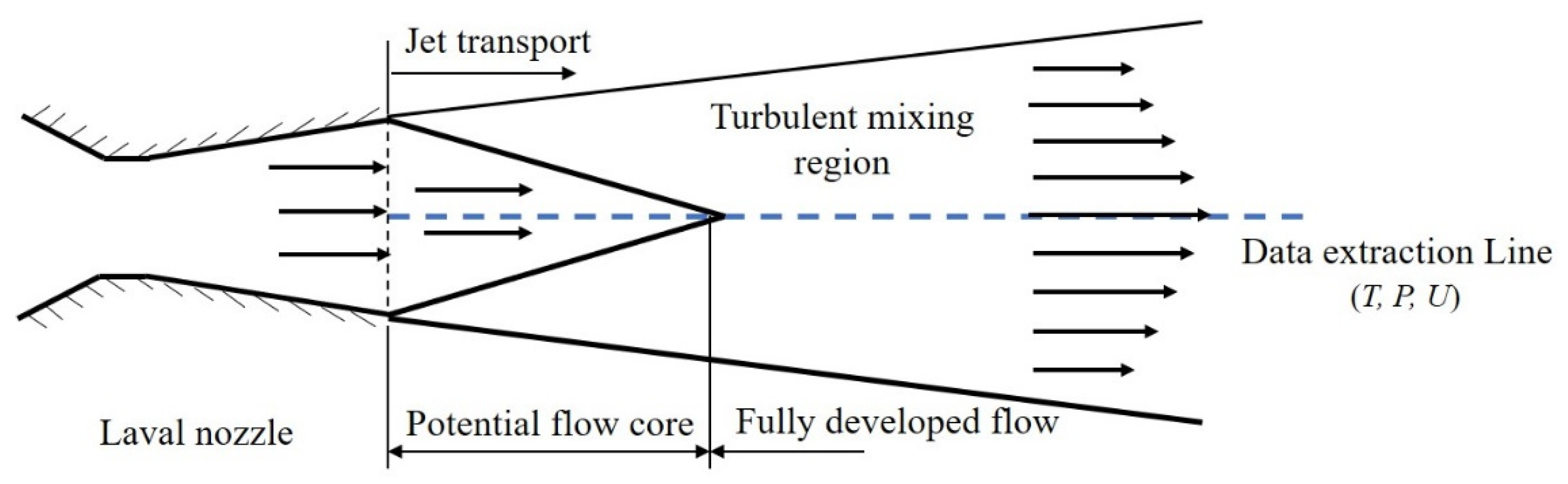
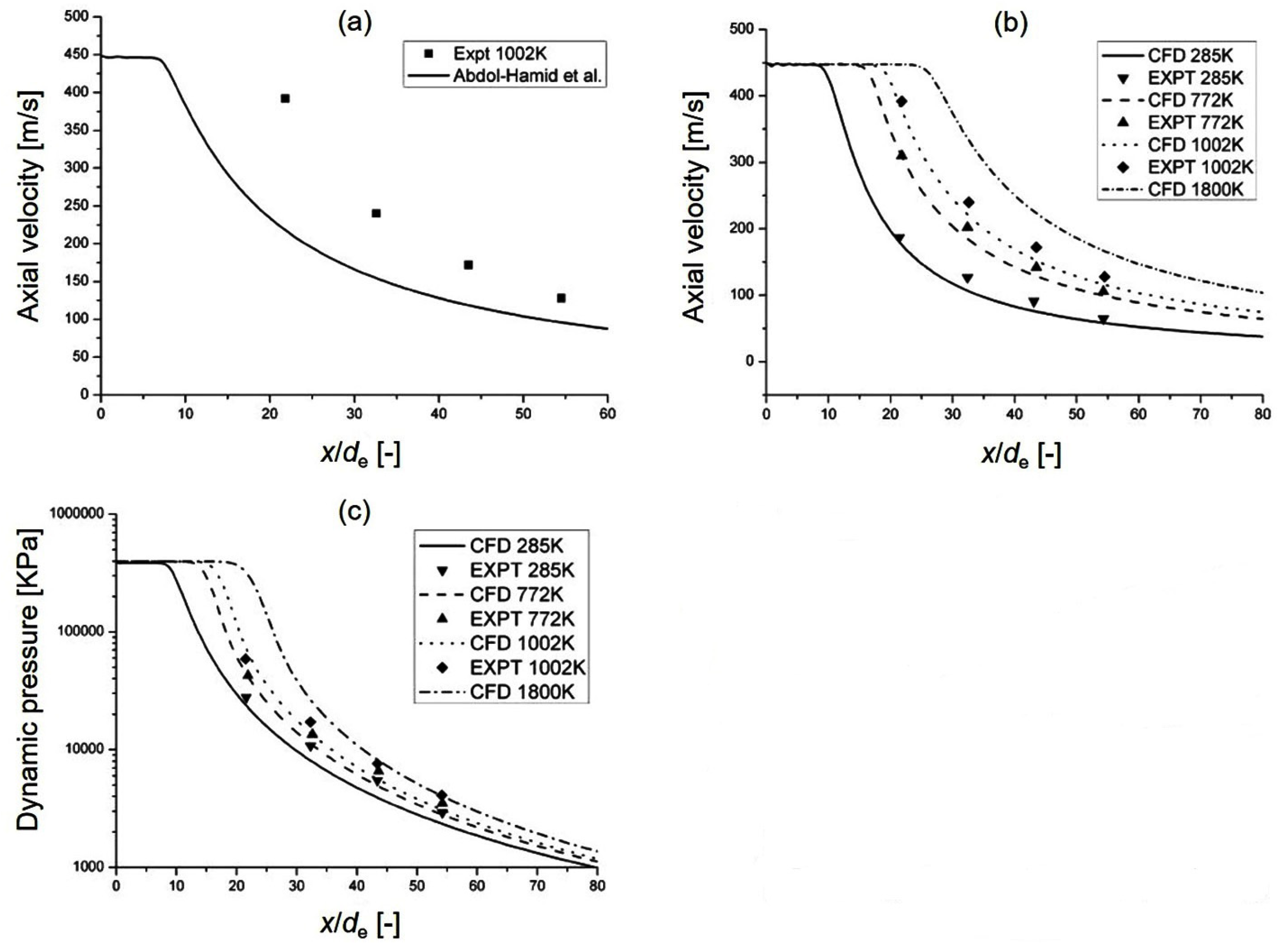
4.2. Supersonic Jet Transport

Supersonic gas jets are applied in Basic Oxygen Furnace (BOF) steelmaking processes [234,235]. Due to its vital role in the refining efficiency [236] and the service lifetime of the furnace lining [237], it is imperative to understand the behavior of the supersonic jet flow. During supersonic jet transport, it interacts with the surrounding medium to produce a turbulent mixing region, as shown in Figure 8. An accurate prediction of the growth rate of the mixing region is a challenge in modelling the jet transport. The standard k-ε turbulence model suffers from a typical weakness, i.e., an overestimated growth rate of the turbulent mixing region around the supersonic gas jet [238]. This leads to a large error in predicting the volume of cavity formed by the gas jet impinging on the liquid surface [239]. Several modifications have been proposed to solve this problem [240,241,242]. Sarkar et al. [240] considered that the compressible dissipation term should be included to account for the effect of the compressibility on the supersonic jet flow. Based on the asymptotic analysis and DNS data, an algebraic model was proposed for the compressible dissipation by using the turbulent Mach number. Subsequently, Sarkar [241] found that the reduced turbulence generation is the main cause of preventing the turbulent mixing layer from the growth rather than the effect of the dilatation term (pressure dilatation and compressible dissipation) on the growth. A gradient Mach number was induced to describe the inhibiting effect of compressibility on the turbulence growth rate. Heinz [242] used the gradient Mach number to evaluate the effect of compressibility on the turbulence distribution. An expression of the model constant C_μ as a function of the gradient Mach number was obtained. However, the k-ε turbulence model with the compressibility correction failed to predict the supersonic jet flow with a temperature gradient, such as the potential flow core length and the cavity shape and dimension [243]. This is because the temperature gradient between the gas jet and the ambient is ignored by the original turbulence model. To sensitize the turbulence model with temperature fluctuation, efforts [244,245,246] have been made to modify the turbulent viscosity term or turbulent heat flux term. Abdol-Hamid et al. [247] corrected the turbulent viscosity term with the temperature gradient for the case of a hot gas jet entering into low temperature ambient. The results of modelling agreed well with experimental data for subsonic and supersonic jet flows. However, this model did not give reasonable results for the BOF supersonic jet flow [243], under which a room temperature gas jet enters into a high temperature ambient (see Figure 9a). Alam et al. [243] modified Abdol-Hamid’s model for the gas jet of BOF. The predicted distributions of axial velocity and dynamic pressure along the central axis of the jet closely agreed with the experimental data (see Figure 9b,c). It is worth mentioning that the data compared in Figure 9 were extracted along the central axis of the jet (see the dashed line in Figure 8). Wang et al. [248] adopted the model of Alam et al. to study the multiple supersonic oxygen jets in the BOF process, where a better prediction of the shape of cavity caused by the gas jet impinging on the liquid surface was achieved. To fit the empirical data available for a cold jet to hot environment [249], Lebon et al. [250] derived another expression of C_μ as a function of the enthalpy ratio of ambient gas to gas jet. It was found that the modified model is adequate to model a compressible jet to hot environment. In addition to the two-equation turbulence model, the LES model with the compressibility and temperature corrections is also widely used to study the jet noises [251]. Wang et al. [252] and Bodony et al. [253] critically reviewed the roles of the SGS model and inflow boundary condition in predicting jet noise. The open issues and future directions were also included in the papers. Therefore, the LES model for jet noise prediction is excluded from this article to avoid repetition.

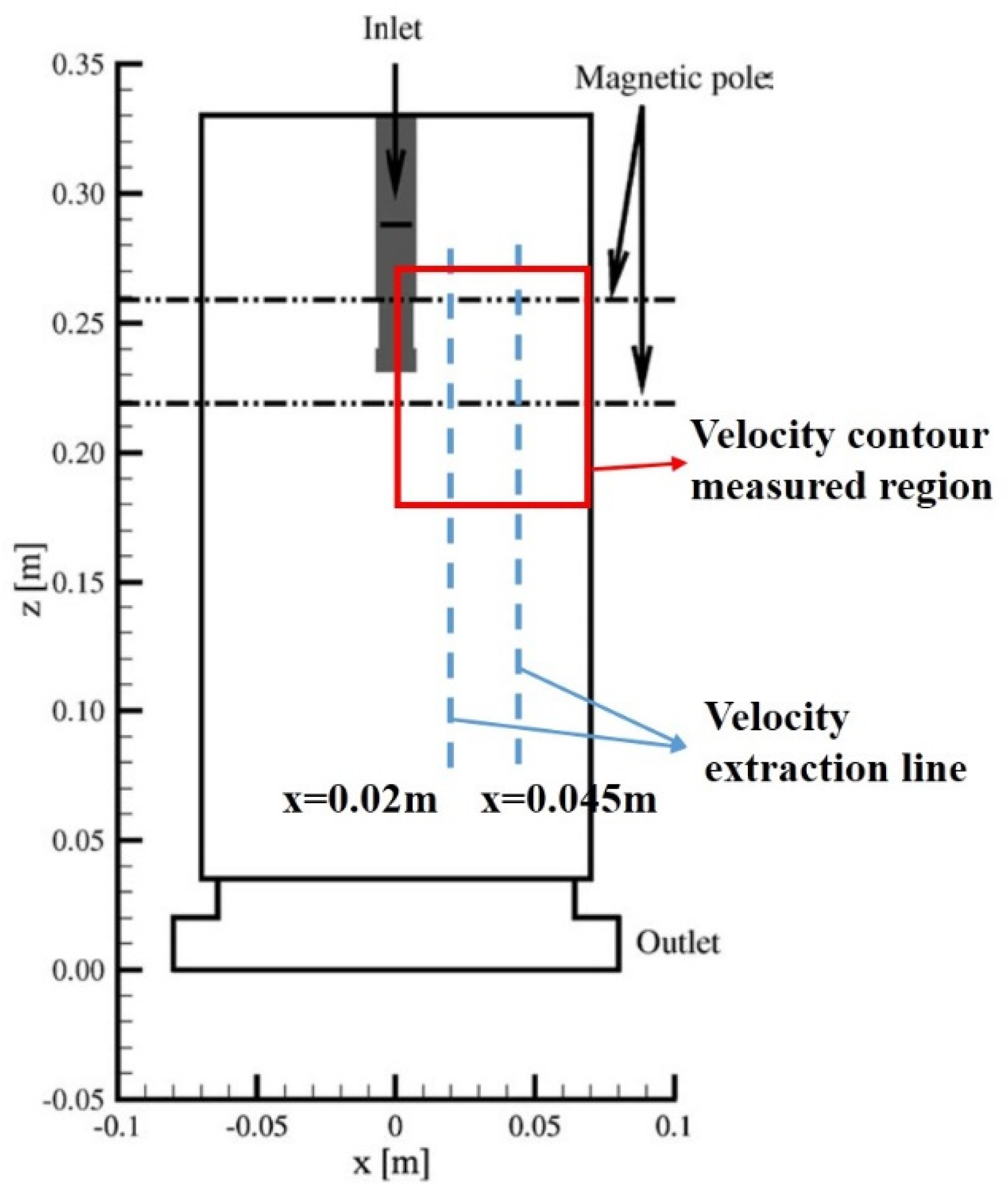
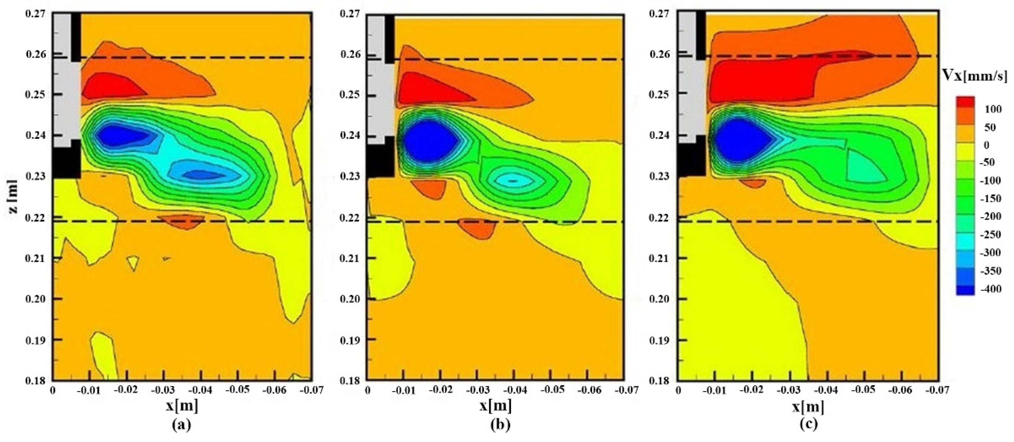
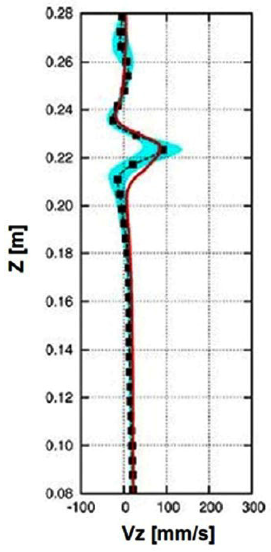
4.3. Electromagnetic Suppression of Turbulence

A static magnetic field has been commonly used to stabilize the turbulent flow in the continuous casting process, aiming to improve the product quality. The application of the magnetic field not only suppresses the mean flow, but also dampens the flow turbulence. For the former, including the electromagnetic force/Lorentz force in the momentum equations, as reported by many studies [254,255,256,257,258], solves the suppression of the mean flow. The latter, also called Joule dissipation, can be resolved by adding the electromagnetic damping effect in a conventional turbulence model. In order to tailor the turbulence model towards magnetohydrodynamic (MHD) flows, many fundamental investigations have been performed [259,260,261,262,263]. Ji and Gardner [259] modified a standard low Re k-ε model [27] to account for the Joule dissipation. Additional source/sink terms were added in the k and ε equations, as well as a damping factor for turbulent viscosity. Both the new terms and the damping factor contain an exponential expression e^−CN, where C is an empirical constant determined from experimental data, and N is the interaction parameter defined as the ratio of the time scale of large eddies (L/U) to the characteristic magnetic braking time (ρ⁄σB²). This interaction parameter represents the strength of turbulence damping due to the magnetic field. However, as reported by Kenjereš and Hanjalić [260], the use of the time scale of large eddies makes the model dependent on the bulk flow properties, restricting the model to homogeneous magnetic fields and simple geometries. Replacing the bulk time scale with the local turbulent time scale (k/ε) can overcome the above-mentioned deficiency. As noted in the work of Ji and Gardner [259], the modified turbulence model failed to accurately predict the turbulent kinetic energy when the strength of the magnetic field increased. This is because the model is formulated based on the assumption of isotropic turbulence, while MHD flows exhibit strong anisotropy caused by the damping of turbulent fluctuations nonparallel to the magnetic field. The anisotropy of the Joule dissipation has to be considered in the turbulence model. Widlund et al. [261] proposed a scalar dimensionality anisotropy parameter carrying the information with regard to the magnitude and anisotropy of the Joule dissipation tensor. A scalar transport equation for the anisotropy parameter was also proposed. With this scalar transport equation, it is easy to extend a conventional turbulence model towards MHD engineering applications. It should be noted that the scalar transport equation is based on phenomenological reasoning, and special attention should be paid to the hydrodynamic part of the proposed equation. Miao et al. [264] coupled the scalar transport equation with the RANS SST k-ω turbulence model [10] to solve the MHD flow in a continuous casting mold. The Joule dissipation was taken into account by adding source/sink terms in the k and ω equations, and the anisotropic behavior of the Joule dissipation was represented by the anisotropy parameter contained in the source/sink terms. The computational domain of the continuous casting mold is shown in Figure 10, and the measured region and data extraction line for liquid metal (low melting point alloy Ga68In20Sn12) velocity are depicted in the figure. The averaged velocities obtained from the three-equation turbulence model (i.e., k-ω-anisotropy parameter) qualitatively and quantitatively agreed with the experimental data (see Figure 11 and Figure 12). The turbulence models described above are modified in the framework of the RANS approach. Due to the time-averaging treatment in the RANS approach, the change of turbulence structure and transient flow behavior are difficult to be captured by the RANS-based turbulence model. Given that engineering flows are usually very complex and have a high Re number, the RANS-based turbulence models are still considered practical candidates for solving MHD flows.

In addition to the RANS-based turbulence model, the LES model, which is able to capture turbulence structures, has been modified or developed to solve the MHD turbulent flow. Shimomura [262] incorporated the magnetic damping effect in the form of a locally determined damping factor for SGS eddy viscosity. Compared with the original Smagorinsky model [12], the new model showed better performance in both turbulent and laminar states. The new model also successfully predicted the anisotropic laminarization caused by the applied magnetic field, for which the RANS-based model is incompetent. Kobayashi [263] developed a new SGS model based on the coherent structure extracted by the second invariant of a velocity gradient tensor in grid scale flow field. Compared with the conventional Smagorinsky model [12], the new SGS model does not need an explicit wall-damping function or change the model parameter depending on the flow. Compared with the dynamic Smagorinsky model [13], the new SGS model is numerically stable due to the fact that the model parameter is always positive. Considering the advantages of the new SGS model, Singh et al. [265,266] used it for the MHD turbulent flow in a continuous caster. The numerical results closely matched the measured data. Although the LES models can capture transient flow behavior and turbulent structures, the computational cost required is much higher than that of the RANS-based turbulence model. With the fast increase in computing power, more LES simulations are expected for engineering flows in the near future. The DNS studies for MHD flows as presented by Chaudhary et al. [267,268] are also necessary since important information regarding turbulent quantities can be obtained for formulating the RANS or LES model. In addition, detailed experiment data, especially the turbulent quantities, are expected for validating numerical simulation of MHD flow.

5. Conclusions

Three main turbulence approaches (i.e., the RANS, LES, and DNS) have been reviewed in this paper. The formulations and variations of the RANS approach have been described, evaluated, and discussed. The eddy viscosity models still remain the most widely used methods for calculating simple engineering flows. The DSM overcomes the limitations of the eddy viscosity model and can be used to predict complex anisotropic flows. However, since a high degree of uncertainty is introduced in the DSM, special attention should be paid to its application. Although the LES is not completely ready for the calculation of high Re number engineering flow in the current stage, it can be used for the studies on fundamental turbulence physics and the low Re number flow in simple geometry. The LES is highly recommended to quantify the turbulent quantities and transient flow behavior. Since the inflow conditions are very important for LES modelling, a further improvement of the method is needed. With the improvement of the model formulation and accurate specification of inlet boundary conditions, the LES shows great potential to realistically solve complex turbulent flows. Due to the high computing power needed, the DNS is often adopted to understand the turbulence physics and to evaluate less advanced turbulence models, rather than being applied for a real case study. It contributes to the development of the turbulence model. Depending on the actual situation, the corresponding experimental validation should be adopted to ensure the fidelity of the used turbulence model before a formal simulation. To demonstrate the application of turbulence modelling, the conventional turbulence models have been customized to resolve three important turbulence-related flow issues, namely, BIT, supersonic jet transport, and electromagnetic damping. Success has been achieved by the customized turbulence model. The general outlook for turbulent flow simulation is listed as follows:

• Due to insufficient knowledge of the turbulence physics, there is a high degree of uncertainty in modelling the higher-order correlations in a DSM simulation. It is necessary to perform fundamental studies on turbulence physics, and the DNS is an important method for those studies. Besides, advanced numerical schemes are expected to minimize the diffusive errors when solving the non-linear higher-order correlations.
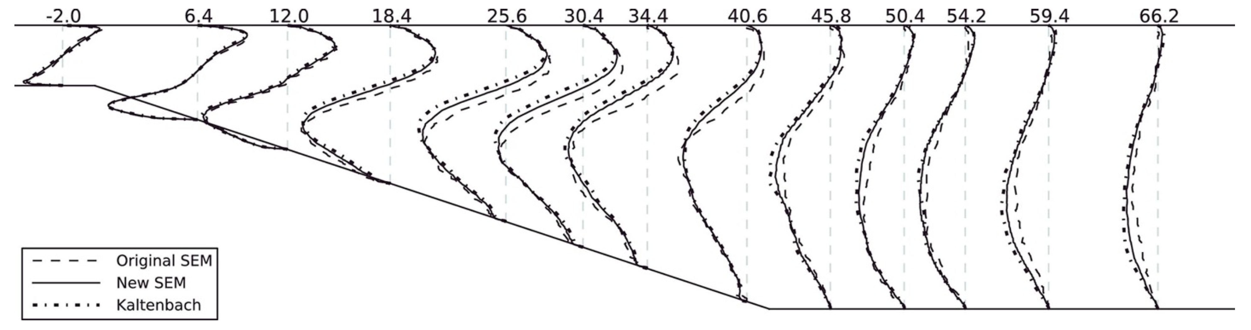
• An inflow condition method, which can generate the required realistic turbulence characteristics at a reasonable computational cost, is needed for an accurate LES simulation.
• It is of significant importance to experimentally obtain accurate turbulence data such as the Reynolds stress term, turbulence kinetic energy, and its dissipation rate, especially for a densely dispersed flow. Advanced non-intrusive experimental techniques are needed to measure the flow field information and phase distribution. The obtained data can be used, for instance, to develop a reliable model considering the effect of the dispersed phase.
• The BIT is important for the turbulent flow. Due to a small size of the bubble, the induced turbulence is characterized with small spatial and temporal scales. An approach (experimental technique and/or numerical simulation) is required to obtain insight into the induced turbulence.
• Comprehensive and realistic modelling is indispensable for engineering applications, such as the inclusion of bubble coalescence and breakage, the consideration of temperature and pressure affecting the bubble behavior, the involvement of compressibility and the temperature gradient in supersonic jet flow, and the turbulence damping caused by magnetic fields. The mechanisms of turbulence modulation with respect to these aspects remain open for fundamental investigation.

References

1. Markatos, N.C. The mathematical modelling of turbulent flows. Appl. Math. Model. 1986, 10, 190–220. [Google Scholar] [CrossRef]
2. Georgiadis, N.J.; Rizzetta, D.P.; Fureby, C. Large-eddy simulation: Current capabilities, recommended practices, and future research. AIAA J. 2010, 48, 1772–1784. [Google Scholar] [CrossRef]
3. Hanjalić, K. Advanced turbulence closure models: A view of current status and future prospects. Int. J. Heat Fluid Flow 1994, 15, 178–203. [Google Scholar] [CrossRef]
4. Argyropoulos, C.D.; Markatos, N.C. Recent advances on the numerical modelling of turbulent flows. Appl. Math. Model. 2015, 39, 693–732. [Google Scholar] [CrossRef]
5. Boris, J.P.; Grinstein, F.F.; Oran, E.S.; Kolbe, R.L. New insights into large eddy simulation. Fluid Dyn. Res. 1992, 10, 199–228. [Google Scholar] [CrossRef]
6. Launder, B.E.; Spalding, D.B. The numerical computation of turbulent flows. Meth. Appl. Mech. Eng. 1974, 3, 269–289. [Google Scholar] [CrossRef]
7. Yakhot, V.; Orszag, S.A. Renormalization group analysis of turbulence: Basic theory. J. Sci. Comput. 1986, 1, 3–51. [Google Scholar] [CrossRef]
8. Shih, T.H.; Liou, W.W.; Shabbir, A.; Yang, Z.; Zhu, J. A new k-ϵ eddy viscosity model for high Reynolds number turbulent flows. Comput. Fluids 1995, 24, 227–238. [Google Scholar] [CrossRef]
9. Wilcox, D.C. Reassessment of the scale-determining equation for advanced turbulence models. AIAA J. 1988, 26, 1299–1310. [Google Scholar] [CrossRef]
10. Menter, F.R. Two-equation eddy-viscosity turbulence models for engineering applications. AIAA J. 1994, 32, 1598–1605. [Google Scholar] [CrossRef] [Green Version]
11. Patel, V.C.; Rodi, W.; Scheuerer, G. Turbulence models for near-wall and low Reynolds number flows—A review. AIAA J. 1985, 23, 1308–1319. [Google Scholar] [CrossRef]
12. Smagorinsky, J. General circulation experiments with the primitive equations. Month. Wea. Rev. 1963, 91, 99–164. [Google Scholar] [CrossRef]
13. Germano, M.; Piomelli, U.; Moin, P.; Cabot, W.H. A dynamic subgrid-scale eddy viscosity model. Phys. Fluids 1991, 3, 1760–1765. [Google Scholar] [CrossRef] [Green Version]
14. Lilly, D.K. A proposed modification of the Germano subgrid-scale closure method. Phys. Fluids 1992, 4, 633–635. [Google Scholar] [CrossRef]
15. Moin, P.; Mahesh, K. Direct numerical simulation: A tool in turbulence Research. Annu. Rev. Fluid Mech. 1998, 30, 539–578. [Google Scholar] [CrossRef] [Green Version]
16. Montorfano, A.; Piscaglia, F.; Ferrari, G. Inlet boundary conditions for incompressible LES: A comparative study. Math. Comput. Model. 2013, 57, 1640–1647. [Google Scholar] [CrossRef]
17. Xie, B.; Gao, F.; Boudet, J.; Shao, L.; Lu, L. Improved vortex method for large-eddy simulation inflow generation. Comput. Fluids 2018, 168, 87–100. [Google Scholar] [CrossRef] [Green Version]
18. Tayebi, D.; Svendsen, H.F.; Jakobsen, H.A.; Grislingas, A. Measurement techniques and data interpretations for validating CFD multiphase reactor models. Chem. Eng. Comm. 2001, 186, 56–159. [Google Scholar] [CrossRef]
19. Van Ommen, J.R.; Mudde, R.F. Measuring the gas-solids distribution in fluidized beds-a review. Int. J. Chem. React. Eng. 2008, 6, 1–29. [Google Scholar] [CrossRef]
20. Hinze, J.O. Turbulence; McGraw-Hill Publishing Co.: New York, NY, USA, 1975. [Google Scholar]
21. Launder, B.E. Second moment closure and its use in modelling turbulent industrial flows. Int. J. Numer. Meth. Fluids 1989, 9, 963–985. [Google Scholar] [CrossRef]
22. Hanjalić, K. Introduction to Turbulence Modelling; Von Kaman Institute for Fluid Dynamics: Sint-Genesius-Rode, Belgium, 2004; pp. 1–75. [Google Scholar]
23. Prandtl, L. Bericht fiber untersuchungen zur ausgebildeten turbulent. ZAMM 1925, 5, 136–139. [Google Scholar] [CrossRef]
24. Spalart, P.R.; Allmaras, S.R. A one-equation turbulence model for aerodynamic flows. In Proceedings of the 30th Aerospace Sciences Meeting and Exhibit, Reno, NV, USA, 6–9 January 1992. [Google Scholar]
25. Nallasamy, M. Turbulence models and their applications to the prediction of internal flows: A review. Comput. Fluids 1987, 15, 151–194. [Google Scholar] [CrossRef]
26. Jones, W.P.; Launder, B.E. The prediction of laminarization with a two-equation model of turbulence. Int. J. Heat Mass Trans. 1972, 15, 301–314. [Google Scholar] [CrossRef]
27. Jones, W.P.; Launder, B.E. The calculation of low-Reynolds-number phenomena with a two-equation model of turbulence. Int. J. Heat Mass Trans. 1973, 16, 1119–1130. [Google Scholar] [CrossRef]
28. Launder, B.E.; Sharma, B.I. Application of the energy-dissipation model of turbulence to the calculation of flow near a spinning disc. Lett. Heat Mass Trans. 1974, 1, 131–138. [Google Scholar] [CrossRef]
29. Hoffmann, G.H. Improved form of the low Reynolds number kε turbulence model. Phys. Fluids 1975, 18, 309–312. [Google Scholar] [CrossRef]
30. Hassid, S.; Poreh, M. A turbulent energy dissipation model for flows with drag reduction. J. Fluids Eng. 1978, 100, 107–112. [Google Scholar] [CrossRef]
31. Lam, C.K.G.; Bremhorst, K. A modified form of the k-ε model for predicting wall turbulence. Tans. ASME 1981, 103, 456–460. [Google Scholar] [CrossRef]
32. Chien, K.Y. Predictions of channel and boundary-layer flows with a low-Reynolds-number turbulence model. AIAA J. 1982, 20, 33–38. [Google Scholar] [CrossRef]
33. Reynolds, W.C. Fundamentals of Turbulence for Turbulence Modeling and Simulation in Lecture Notes for Von Karman Institute; AGARD Lecture Note Series: New York, NY, USA, 1987. [Google Scholar]
34. Shih, T.H.; Zhu, J.; Lumley, J.L. A new Reynolds stress algebraic model. NASA TM 1995, 125, 1–4. [Google Scholar]
35. Menter, F.R. Review of the shear-stress transport turbulence model experience from an industrial perspective. Int. J. Comput. Fluid Dyn. 2009, 23, 305–316. [Google Scholar] [CrossRef]
36. Wilcox, D.C. Comparison of two-equation turbulence models for boundary layers with pressure gradient. AIAA J. 1993, 31, 1414–1421. [Google Scholar] [CrossRef]
37. Wilcox, D.C. Simulation of transition with a two-equation turbulence model. AIAA J. 1994, 32, 247–255. [Google Scholar] [CrossRef]
38. Peng, S.H.; Davidson, L.; Holmberg, S. A modified low-Reynolds-number k-ω model for recirculating flows. J. Fluid Eng. 1997, 119, 867–875. [Google Scholar] [CrossRef]
39. Bredberg, J.; Peng, S.H.; Davidson, L. An improved k-ω turbulence model applied to recirculating flows. Int. J. Heat Fluid Flow 2002, 23, 731–743. [Google Scholar] [CrossRef]
40. Resende, P.R.; Pinho, F.T.; Younis, B.A.; Kim, K.; Sureshkumar, R. Development of a low-Reynolds-number k-ω model for FENE-P fluids. Flow Turbul. Combust. 2013, 90, 69–94. [Google Scholar] [CrossRef]
41. Durbin, P.A. Near-wall turbulence closure modeling without “damping functions”. Theor. Comput. Fluid Dyn. 1991, 3, 1–13. [Google Scholar]
42. Durbin, P.A. On the k-ε stagnation point anomaly. Int. J. Heat Fluid Flow 1996, 17, 89–90. [Google Scholar] [CrossRef]
43. Laurence, D.R.; Uribe, J.C.; Utyuzhnikov, S.V. A robust formulation of the v2−f model. Flow Turb. Combust. 2004, 73, 169–185. [Google Scholar] [CrossRef] [Green Version]
44. Hanjalić, K.; Popovac, M.; Hadžiabdić, M. A robust near-wall elliptic-relaxation eddy-viscosity turbulence model for CFD. Int. J. Heat Fluid Flow 2004, 25, 1047–1051. [Google Scholar] [CrossRef]
45. Billard, F.; Laurence, D. A robust k-ε v ¯ 2k elliptic blending turbulence model applied to near-wall, separated and buoyant flows. Int. J. Heat Fluid Flow 2012, 33, 45–58. [Google Scholar] [CrossRef]
46. Billard, F.; Revell, A.; Craft, T. Application of recently developed elliptic blending based models to separated flows. Int. J. Heat Fluid Flow 2012, 35, 141–151. [Google Scholar] [CrossRef]
47. Speziale, C.G. On nonlinear kl and k-ε models of turbulence. J. Fluid Mech. 1987, 178, 459–475. [Google Scholar] [CrossRef]
48. Lien, F.S.; Leschziner, M.A. Assessment of turbulence-transport models including non-linear RNG eddy-viscosity formulation and second-moment closure for flow over a backward-facing step. Comput. Fluids 1994, 23, 983–1004. [Google Scholar] [CrossRef]
49. Craft, T.J.; Launder, B.E.; Suga, K. Development and application of a cubic eddy-viscosity model of turbulence. Int. J. Heat Fluid Flow 1996, 17, 08–115. [Google Scholar] [CrossRef]
50. Craft, T.J.; Launder, B.E.; Suga, K. Prediction of turbulent transitional phenomena with a nonlinear eddy-viscosity model. Int. J. Heat Fluid Flow 1997, 18, 15–28. [Google Scholar] [CrossRef]
51. Apsley, D.D.; Leschziner, M.A. A new low-Reynolds-number nonlinear two-equation turbulence model for complex flows. Int. J. Heat Fluid Flow 1998, 19, 209–222. [Google Scholar] [CrossRef]
52. Jongen, T.; Machiels, L.; Gatski, T.B. Predicting noninertial effects with linear and nonlinear eddy-viscosity, and algebraic stress models. Flow Turb. Combust. 1998, 60, 215–234. [Google Scholar] [CrossRef]
53. Hellsten, A.; Wallin, S. Explicit algebraic Reynolds stress and non-linear eddy-viscosity models. Int. J. Comput. Fluid Dyn. 2009, 23, 349–361. [Google Scholar] [CrossRef]
54. Gatski, T.B.; Speziale, C.G. On explicit algebraic stress models for complex turbulent flows. J. Fluid Mech. 1993, 254, 59–78. [Google Scholar] [CrossRef] [Green Version]
55. Gatski, T.B.; Jongen, T. Nonlinear eddy viscosity and algebraic stress models for solving complex turbulent flows. Prog. Aerosp. Sci. 2000, 36, 655–682. [Google Scholar] [CrossRef]
56. Gatski, T.B.; Wallin, S. Extending the weak-equilibrium condition for algebraic Reynolds stress models to rotating and curved flows. J. Fluid Mech. 2004, 518, 147–155. [Google Scholar] [CrossRef]
57. Rodi, W. The Prediction of Free Turbulent Shear Flows by Use of a 2-Equation Model of Turbulence. Ph.D. Thesis, University of London, London, UK, 1972. [Google Scholar]
58. Rodi, W. A new algebraic relation for calculating the Reynolds stresses. ZAMM 1976, 56, 219–221. [Google Scholar] [CrossRef]
59. Kim, J.; Moin, P.; Moser, R. Turbulence statistics in fully developed channel flow at low Reynolds number. J. Fluid Mech. 1987, 177, 133–166. [Google Scholar] [CrossRef] [Green Version]
60. Daly, B.J.; Harlow, F.H. Transport equations in turbulence. Phys. Fluids 1970, 13, 2634–2649. [Google Scholar] [CrossRef]
61. Hanjalić, K.; Launder, B.E. A Reynolds stress model of turbulence and its application to thin shear flows. J. Fluid Mech. 1972, 52, 609–638. [Google Scholar] [CrossRef]
62. Shir, C.C. A preliminary numerical study of atmospheric turbulent flows in the idealized planetary boundary layer. J. Atmospher. Sci. 1973, 30, 1327–1339. [Google Scholar] [CrossRef] [Green Version]
63. Mellor, G.L.; Herring, H.J. A survey of the mean turbulent field closure models. AIAA J. 1973, 11, 590–599. [Google Scholar] [CrossRef]
64. Nagano, Y.; Tagawa, M. Turbulence model for triple velocity and scalar correlations. In Turbulent Shear Flows 7; Springer: Berlin, Germany, 1991; Volume 7, pp. 47–62. [Google Scholar]
65. Magnaudet, J. The modelling of inhomogeneous turbulence in the absence of mean velocity gradients. In Proceedings of the 4th European Turbulence Conference, Delft, The Netherlands, 30 June–3 July 1992. [Google Scholar]
66. Launder, B.E. Phenomenological modelling: Present and future? In Proceedings of the Workshop Held at Cornell University, Ithaca, NY, USA, 22–24 March 1989. [Google Scholar]
67. Rotta, J.C. Statistische Theorie nichthomogener Turbulenz. Z. Phys. 1951, 129, 547–572. [Google Scholar] [CrossRef]
68. Lumley, J.L. Computational modeling of turbulent flows. Adv. Appl. Mech. 1979, 18, 123–176. [Google Scholar]
69. Naot, D. Interactions between components of the turbulent velocity correlation tensor. Isr. J. Technol. 1970, 8, 259–269. [Google Scholar]
70. Launder, B.E.; Reece, G.J.; Rodi, W. Progress in the development of a Reynolds-stress turbulence closure. J. Fluid Mech. 1975, 68, 537–566. [Google Scholar] [CrossRef] [Green Version]
71. Speziale, C.G.; Sarkar, S.; Gatski, T.B. Modelling the pressure-strain correlation of turbulence: An invariant dynamical systems approach. J. Fluid Mech. 1991, 227, 245–272. [Google Scholar] [CrossRef]
72. Shih, T.H.; Lumley, J.L. Modeling of Pressure Correlation Terms in Reynolds Stress and Scalar Flux Equations; Cornell University: Ithaca, NY, USA, 1985. [Google Scholar]
73. Craft, T.J.; Launder, B.E. Computation of impinging flows using second-moment closures. In Proceedings of the 8th Symposium on Turbulent Shear Flows, Munich, Germany, 9–11 September 1991; pp. 851–856. [Google Scholar]
74. Launder, B.E.; Tselepidakis, D.P. Progress and paradoxes in modelling near-wall turbulence. In Proceedings of the 8th Symposium on Turbulent Shear Flows, Munich, Germany, 9–11 September 1991; pp. 2911–2916. [Google Scholar]
75. Gibson, M.M.; Launder, B.E. Ground effects on pressure fluctuations in the atmospheric boundary layer. J. Fluid Mech. 1978, 86, 491–511. [Google Scholar] [CrossRef]
76. Durbin, P.A. A Reynolds stress model for near-wall turbulence. J. Fluid Mech. 1993, 249, 465–498. [Google Scholar] [CrossRef]
77. Manceau, R.; Hanjalić, K. Elliptic blending model: A new near-wall Reynolds-stress turbulence closure. Phys. Fluids 2002, 14, 744–754. [Google Scholar] [CrossRef]
78. Leonard, A. Energy cascade in large-eddy simulations of turbulent fluid flows. Adv. Geophys. 1975, 18, 237–248. [Google Scholar]
79. Nicoud, F.; Ducros, F. Subgrid-scale stress modelling based on the square of the velocity gradient tensor. Flow Turb. Combust. 1999, 62, 183–200. [Google Scholar] [CrossRef]
80. Schumann, U. Subgrid scale model for finite difference simulations of turbulent flows in plane channels and annuli. J. Comput. Phys. 1975, 18, 376–404. [Google Scholar] [CrossRef] [Green Version]
81. Piomelli, U. High Reynolds number calculations using the dynamic subgrid-scale stress model. Phys. Fluids 1993, 5, 1484–1490. [Google Scholar] [CrossRef]
82. Kim, W.W.; Menon, S. A new dynamic one-equation subgrid-scale model for large eddy simulations. In Proceedings of the AIAA 34th Aerospace Sciences Meeting and Exhibit, Reno, NV, USA, 15–18 January 1996. [Google Scholar]
83. Kajishima, T.; Nomachi, T. One-equation subgrid scale model using dynamic procedure for the energy production. J. Appl. Mech. 2006, 73, 368–373. [Google Scholar] [CrossRef]
84. Huang, S.; Li, Q.S. A new dynamic one equation subgrid scale model for large eddy simulations. Int. J. Numer. Meth. Eng. 2010, 81, 835–865. [Google Scholar] [CrossRef]
85. Shur, M.L.; Spalart, P.R.; Strelets, M.K.; Travin, A.K. A hybrid RANS-LES approach with delayed-DES and wall-modelled LES capabilities. Int. J. Heat Fluid Flow 2008, 29, 1638–1649. [Google Scholar] [CrossRef]
86. Piomelli, U.; Moin, P.; Ferziger, J.H. Model consistency in large eddy simulation of turbulent channel flows. Phys. Fluids 1988, 31, 884–1891. [Google Scholar] [CrossRef]
87. Vreman, A.W. An eddy-viscosity subgrid-scale model for turbulent shear flow: Algebraic theory and applications. Phys. Fluids 2004, 16, 3670–3681. [Google Scholar] [CrossRef]
88. Verstappen, R.W.C.P.; Bose, S.T.; Lee, J.; Choi, H.; Moin, P. A dynamic eddy-viscosity model based on the invariants of the rate-of-strain. In Proceedings of the Summer Program of the Center for Turbulence Research, Stanford, CA, USA, 2010; pp. 183–192. [Google Scholar]
89. Verstappen, R.W.C.P. When does eddy viscosity damp subfilter scales sufficiently? J. Sci. Comput. 2011, 49, 94–110. [Google Scholar] [CrossRef] [Green Version]
90. Nicoud, F.; Toda, H.B.; Cabrit, O.; Bose, S.; Lee, J. Using singular values to build a subgrid-scale model for large eddy simulations. Phys. Fluids 2011, 23, 085106. [Google Scholar] [CrossRef] [Green Version]
91. Trias, F.X.; Folch, D.; Gorobets, A.; Oliva, A. Building proper invariants for eddy-viscosity subgrid-scale models. Phys. Fluids 2015, 27, 065103. [Google Scholar] [CrossRef] [Green Version]
92. Park, N.; Lee, S.; Lee, J.; Choi, H. A dynamic subgrid-scale eddy viscosity model with a global model coefficient. Phys. Fluids 2006, 18, 125109. [Google Scholar] [CrossRef]
93. You, D.; Moin, P. A dynamic global-coefficient subgrid-scale eddy-viscosity model for large-eddy simulation in complex geometries. Phys. Fluids 2007, 19, 065110. [Google Scholar] [CrossRef] [Green Version]
94. Lee, J.; Choi, H.; Park, N. Dynamic global model for large eddy simulation of transient flow. Phys. Fluids 2010, 22, 075106. [Google Scholar] [CrossRef]
95. Rozema, W.; Bae, H.J.; Moin, P.; Verstappen, R. Minimum-dissipation models for large-eddy simulation. Phys. Fluids 2015, 27, 085107. [Google Scholar] [CrossRef] [Green Version]
96. Rieth, M.; Proch, F.; Stein, O.T.; Pettit, M.W.A.; Kempf, A.M. Comparison of the Sigma and Smagorinsky LES models for grid generated turbulence and a channel flow. Comput. Fluids 2014, 99, 172–181. [Google Scholar] [CrossRef]
97. Bardina, J.; Ferziger, J.H.; Reynolds, W.C. Improved subgrid-scale models for large-eddy simulation. In Proceedings of the AlAA 13th Fluid and Plasma Dynamics Coference, Colorado, CO, USA, 14–16 July 1980. [Google Scholar]
98. Liu, S.; Meneveau, C.; Katz, J. On the properties of similarity subgrid-scale models as deduced from measurements in a turbulent jet. J. Fluid Mech. 1994, 275, 83–119. [Google Scholar] [CrossRef]
99. Liu, S.; Meneveau, C.; Katz, J. Experimental study of similarity subgrid-scale models of turbulence in the far-field of a jet. Appl. Sci. Res. 1995, 54, 177–190. [Google Scholar] [CrossRef]
100. Akhavan, R.; Ansari, A.; Kang, S.; Mangiavacchi, N. Subgrid-scale interactions in a numerically simulated planar turbulent jet and implications for modelling. J. Fluid Mech. 2000, 408, 83–120. [Google Scholar] [CrossRef]
101. Domaradzki, J.A.; Saiki, E.M. A subgrid-scale model based on the estimation of unresolved scales of turbulence. Phys. Fluids. 1997, 9, 2148–2164. [Google Scholar] [CrossRef]
102. Domaradzki, J.A.; Loh, K.C. The subgrid-scale estimation model in the physical space representation. Phys. Fluids 1999, 11, 2330–2342. [Google Scholar] [CrossRef]
103. Stolz, S.; Adams, N.A. An approximate deconvolution procedure for large-eddy simulation. Phys. Fluids 1999, 11, 1699–1701. [Google Scholar] [CrossRef]
104. Stolz, S.; Adams, N.A.; Kleiser, L. An approximate deconvolution model for large-eddy simulation with application to incompressible wall-bounded flows. Phys. Fluids 2001, 13, 997–1015. [Google Scholar] [CrossRef]
105. Stolz, S.; Adams, N.A.; Kleiser, L. The approximate deconvolution model for large-eddy simulations of compressible flows and its application to shock-turbulent-boundary-layer interaction. Phys. Fluids 2001, 13, 2985–3001. [Google Scholar] [CrossRef]
106. Geurts, B.J.; Holm, D.D. Regularization modeling for large-eddy simulation. Phys. Fluids 2003, 15, 13–16. [Google Scholar] [CrossRef] [Green Version]
107. Cheskidov, A.; Holm, D.D.; Olson, E.; Titi, E.S. On a Leray-α model of turbulence. Proc. R. Soc. 2005, 461, 629–649. [Google Scholar] [CrossRef]
108. Cao, C.; Holm, D.D.; Titi, E.S. On the Clark-α model of turbulence: Global regularity and long-time dynamics. J. Turb. 2005, 6, 1–11. [Google Scholar] [CrossRef] [Green Version]
109. Stolz, S.; Adams, N.A. Large-eddy simulation of high-Reynolds-number supersonic boundary layers using the approximate deconvolution model and a rescaling and recycling technique. Phys. Fluids 2003, 15, 2398–2412. [Google Scholar] [CrossRef]
110. Schlatter, P.; Stolz, S.; Kleiser, L. LES of transitional flows using the approximate deconvolution model. Int. J. Heat Fluid Flow 2004, 25, 549–558. [Google Scholar] [CrossRef]
111. Saeedipour, M.; Vincent, S.; Pirker, S. Large eddy simulation of turbulent interfacial flows using approximate deconvolution model. Int. J. Multiph. Flow 2019, 112, 286–299. [Google Scholar] [CrossRef]
112. Ilyin, A.A.; Lunasin, E.M.; Titi, E.S. A modified-Leray-α subgrid scale model of turbulence. Nonlinearity 2006, 19, 879–897. [Google Scholar] [CrossRef]
113. Foias, C.; Holm, D.D.; Titi, E.S. The Navier-stokes-alpha model of fluid turbulence. Phys. D 2001, 152–153, 505–519. [Google Scholar] [CrossRef] [Green Version]
114. Rebholz, L.G. A family of new, high order NS-α models arising from helicity correction in Leray turbulence models. J. Math. Anal. Appl. 2008, 342, 246–254. [Google Scholar] [CrossRef] [Green Version]
115. Layton, W.; Rebholz, L.; Sussman, M. Energy and helicity dissipation rates of the NS-alpha and NS-alpha-deconvolution models. J. Appl. Math. 2010, 75, 56–74. [Google Scholar] [CrossRef] [Green Version]
116. Rebholz, L.G.; Sussman, M.M. On the high accuracy NS-alpha-deconvolution turbulence model. Math. Models Methods Appl. Sci. 2010, 20, 611–633. [Google Scholar] [CrossRef]
117. Breckling, S.; Neda, M. Numerical study of the Navier–Stokes-α deconvolution model with pointwise mass conservation. Int. J. Comput. Math. 2018, 95, 1727–1760. [Google Scholar] [CrossRef]
118. Cuff, V.M.; Dunca, A.A.; Monica, C.C.; Rebholz, L.G. The reduced order NS-α model for incompressible flow: Theory, numerical analysis and benchmark testing. Math. Modell. Numer. Anal. 2015, 49, 641–662. [Google Scholar] [CrossRef]
119. Bowers, A.L.; Rebholz, L.G. The reduced NS-α model for incompressible flow: A review of recent progress. Fluids 2017, 38, 38. [Google Scholar] [CrossRef]
120. Geurts, B.J.; Kuczaj, A.K.; Titi, E.S. Regularization modeling for large-eddy simulation of homogeneous isotropic decaying turbulence. J. Phys. Math. Theor. 2008, 41, 344008. [Google Scholar] [CrossRef]
121. Graham, J.P.; Holm, D.D.; Mininni, P.D.; Pouquet, A. Three regularization models of the navier-stokes equations. Phys. Fluids 2008, 20, 035107. [Google Scholar] [CrossRef] [Green Version]
122. Sheu, T.W.H.; Lin, Y.X.; Yu, C.H. Numerical study of two regularization models for simulating the turbulent flows. Comput. Fluids 2013, 74, 13–31. [Google Scholar] [CrossRef]
123. Huai, X.; Joslin, R.D.; Piomelli, U. Large-eddy simulation of transition to turbulence in boundary layers. Theor. Comput. Fluid Dyn. 1997, 9, 149–163. [Google Scholar] [CrossRef] [Green Version]
124. Yang, Z.; Voke, P.R. Large-eddy simulation of boundary-layer separation and transition at a change of surface curvature. J. Fluid Mech. 2001, 439, 305–333. [Google Scholar] [CrossRef]
125. Sayadi, T.; Moin, P. Large eddy simulation of controlled transition to turbulence. Phys. Fluids 2012, 24, 114103. [Google Scholar] [CrossRef]
126. Langari, M.; Yang, Z. Numerical study of the primary instability in a separated boundary layer transition under elevated free-stream turbulence. Phys. Fluids 2013, 25, 074106. [Google Scholar] [CrossRef] [Green Version]
127. Mittal, R.; Moin, P. Suitability of upwind-biased finite difference schemes for large-eddy simulation of turbulent flows. AIAA J. 1997, 35, 1415–1417. [Google Scholar] [CrossRef]
128. Kravchenko, A.G.; Moin, P. Numerical studies of flow over a circular cylinder at ReD = 3900. Phys. Fluids 2000, 12, 403–417. [Google Scholar] [CrossRef]
129. Dhotre, M.T.; Niceno, B.; Smith, B.L. Large eddy simulation of a bubble column using dynamic sub-grid scale model. Chem. Eng. J. 2008, 136, 337–348. [Google Scholar] [CrossRef]
130. Wang, Y.; Vanierschot, M.; Cao, L.; Cheng, Z.; Blanpain, B.; Guo, M. Hydrodynamics study of bubbly flow in a top-submerged lance vessel. Chem. Eng. Sci. 2018, 192, 1091–1104. [Google Scholar] [CrossRef]
131. Nilsen, K.M.; Kong, B.; Fox, R.O.; Hill, J.C.; Olsen, M.G. Effect of inlet conditions on the accuracy of large eddy simulations of a turbulent rectangular wake. Chem. Eng. J. 2014, 250, 175–189. [Google Scholar] [CrossRef]
132. Spille-Kohoff, A.; Kaltenbach, H.J. Generation of turbulent inflow data with a prescribed shear-stress profile. In Proceedings of the 3rd AFOSR International conference on DNS/LES, Arlington, TX, USA, 5–9 August 2001. [Google Scholar]
133. Baba-Ahmadi, M.H.; Tabor, G.R. Inlet conditions for LES using mapping and feedback control. Comput. Fluids 2009, 38, 1299–1311. [Google Scholar] [CrossRef] [Green Version]
134. Baba-Ahmadi, M.H.; Tabor, G.R. Inlet conditions for large eddy simulation of gas-turbine swirl injectors. AIAA J. 2008, 46, 1782–1790. [Google Scholar] [CrossRef] [Green Version]
135. Aider, J.L.; Danet, A.; Lesieur, M. Large-eddy simulation applied to study the influence of upstream conditions on the time-dependant and averaged characteristics of a backward-facing step flow. J. Turb. 2007, 8, 1–30. [Google Scholar] [CrossRef]
136. Batten, P.; Goldberg, U.; Chakravarthy, S. Interfacing statistical turbulence closures with large-eddy simulation. AIAA J. 2004, 42, 485–492. [Google Scholar] [CrossRef]
137. Andersson, N.; Eriksson, L.E.; Davidson, L. LES prediction of flow and acoustic field of a coaxial jet. In Proceedings of the 11th AIAA/CES Aeroacoustics Conference, Monterey, CA, USA, 23–25 May 2005. [Google Scholar]
138. Druault, P.; Lardeau, S.; Bonnet, J.P.; Coiffet, F.; Delville, J.; Lamballais, E.; Largeau, J.F.; Perret, L. Generation of three-dimensional turbulent inlet conditions for large-eddy simulation. AIAA J. 2004, 42, 447–456. [Google Scholar] [CrossRef]
139. Perret, L.; Delville, J.; Manceau, R.; Bonnet, J.P. Turbulent inflow conditions for large-eddy simulation based on low-order empirical model. Phys. Fluids 2008, 20, 075107. [Google Scholar] [CrossRef]
140. Klein, M.; Sadiki, A.; Janicka, J. A digital filter based generation of inflow data for spatially developing direct numerical or large eddy simulations. J. Comput. Phys. 2003, 186, 652–665. [Google Scholar] [CrossRef]
141. Di Mare, L.; Klein, M.; Jones, W.P.; Janicka, J. Synthetic turbulence inflow conditions for large-eddy simulation. Phys. Fluids 2006, 18, 025107. [Google Scholar] [CrossRef]
142. Jarrin, N.; Benhamadouche, S.; Laurence, D.; Prosser, R. A synthetic-eddy-method for generating inflow conditions for large-eddy simulations. Int. J. Heat Fluid Flow 2006, 27, 585–593. [Google Scholar] [CrossRef] [Green Version]
143. Jarrin, N.; Prosser, R.; Uribe, J.C.; Benhamadouche, S.; Laurence, D. Reconstruction of turbulent fluctuations for hybrid RANS/LES simulations using a synthetic-eddy method. Int. J. Heat Fluid Flow 2009, 30, 435–442. [Google Scholar] [CrossRef] [Green Version]
144. Skillen, A.; Revell, A.; Craft, T. Accuracy and efficiency improvements in synthetic eddy methods. Int. J. Heat Fluid Flow 2016, 62, 386–394. [Google Scholar] [CrossRef]
145. Keating, A.; Piomelli, U.; Balaras, E.; Kaltenbach, H.J. A priori and a posteriori tests of inflow conditions for large-eddy simulation. Phys. Fluids 2004, 16, 4696–4712. [Google Scholar] [CrossRef]
146. Benhamadouche, S.; Jarrin, N.; Addad, Y.; Laurence, D. Synthetic turbulent inflow conditions based on a vortex method for large-eddy simulation. Prog. Comput. Fluid Dyn. 2006, 6, 50–57. [Google Scholar] [CrossRef]
147. Kaltenbach, H.J.; Fatica, M.; Mittal, R.; Lund, T.S.; Moin, P. Study of flow in a planar asymmetric diffuser using large-eddy simulation. J. Fluid Mech. 1999, 390, 151–185. [Google Scholar] [CrossRef]
148. Kasagi, N.; Shikazono, N. Contribution of direct numerical simulation to understanding and modelling turbulent transport. Proc. R. Soc. Lond. 1995, 451, 257–292. [Google Scholar]
149. Kim, J.W.; Sandberg, R.D. Efficient parallel computing with a compact finite difference scheme. Comput. Fluids 2012, 58, 70–87. [Google Scholar] [CrossRef]
150. Alfonsi, G.; Ciliberti, S.A.; Mancini, M.; Primavera, L. Performances of navier-stokes solver on a hybrid cpu/gpu computing system. In Proceedings of the International Conference on Parallel Computing Techonologies, Berlin/Heidelberg, Germany, 19–23 September 2011; pp. 404–416. [Google Scholar]
151. Alfonsi, G.; Ciliberti, S.A.; Mancini, M.; Primavera, L. Direct numerical simulation of turbulent channel flow on high-performance GPU computing system. Computation 2016, 4, 13. [Google Scholar] [CrossRef] [Green Version]
152. Alfonsi, G.; Ciliberti, S.A.; Mancini, M.; Primavera, L. GPGPU implementation of mixed spectral-finite difference computational code for the numerical integration of the three-dimensional time-dependent incompressible Navier–Stokes equations. Comput. Fluids 2014, 102, 237–249. [Google Scholar] [CrossRef]
153. Laizet, S.; Lamballais, E.; Vassilicos, J.C. A numerical strategy to combine high-order schemes, complex geometry and parallel computing for high resolution DNS of fractal generated turbulence. Comput. Fluids 2010, 39, 471–484. [Google Scholar] [CrossRef]
154. Alfonsi, G. On direct numerical simulation of turbulent flows. Appl. Mech. Rev. 2011, 64, 020802. [Google Scholar] [CrossRef]
155. Feng, J.; Bolotnov, I.A. Evaluation of bubble-induced turbulence using direct numerical simulation. Int. J. Multiph. Flow 2017, 93, 92–107. [Google Scholar] [CrossRef] [Green Version]
156. Abe, H.; Kawamura, H.; Matsuo, Y. Direct numerical simulation of a fully developed turbulent channel flow with respect to the Reynolds number dependence. J. Fluids Eng. 2001, 123, 382–393. [Google Scholar] [CrossRef]
157. Pirozzoli, S.; Grasso, F.; Gatski, T.B. Direct numerical simulation and analysis of a spatially evolving supersonic turbulent boundary layer at M = 2.25. Phys. Fluids 2004, 16, 530–545. [Google Scholar] [CrossRef]
158. Ma, M.; Lu, J.; Tryggvason, G. Using statistical learning to close two-fluid multiphase flow equations for a simple bubbly system. Phys. Fluids 2015, 27, 092101. [Google Scholar] [CrossRef]
159. Fang, J.; Cambareri, J.J.; Brown, C.S.; Feng, J.; Gouws, A.; Li, M.; Bolotnov, I.A. Direct numerical simulation of reactor two-phase flows enabled by high-performance computing. Nucl. Eng. Des. 2018, 330, 409–419. [Google Scholar] [CrossRef]
160. Singhal, A.; Cloete, S.; Radl, S.; Quinta-Ferreira, R.; Amini, S. Heat transfer to a gas from densely packed beds of monodisperse spherical particles. Chem. Eng. J. 2017, 314, 27–37. [Google Scholar] [CrossRef]
161. Feng, X.; Yang, C.; Mao, Z.S.; Lu, J.; Tryggvason, G. Bubble induced turbulence model improved by direct numerical simulation of bubbly flow. Chem. Eng. J. 2019, 377, 120001. [Google Scholar] [CrossRef]
162. Feng, J.; Bolotnov, I.A. Interfacial force study on a single bubble in laminar and turbulent flows. Nucl. Eng. Des. 2017, 313, 345–360. [Google Scholar] [CrossRef] [Green Version]
163. Suzuki, Y.; Kasagi, N. Evaluation of hot-wire measurements in wall shear turbulence using a direct numerical simulation database. Exp. Therm. Fluid Sci. 1992, 5, 69–77. [Google Scholar] [CrossRef]
164. Tang, Y.; Lau, Y.M.; Deen, N.G.; Peters, E.A.J.F.; Kuipers, J.A.M. Direct numerical simulations and experiments of a pseudo-2D gas-fluidized bed. Chem. Eng. Sci. 2016, 143, 166–180. [Google Scholar] [CrossRef]
165. Werther, J.; Hage, B.; Rudnick, C. A comparison of laser Doppler and single-fiber reflection probes for the measurement of the velocity of solids in a gas-solid circulating fluidized bed. Chem. Eng. Process. 1996, 35, 381–391. [Google Scholar] [CrossRef]
166. Zhang, M.; Qian, Z.; Yu, H.; Wei, F. The solid flow structure in a circulating fluidized bed riser/downer of 0.42-m diameter. Powder Technol. 2003, 129, 46–52. [Google Scholar] [CrossRef]
167. Link, J.; Zeilstra, C.; Deen, N.G.; Kuipers, J.A.M. Validation of a discrete particle model in a 2D spout-fluid bed using non intrusive optical measuring techniques. Can. J. Chem. Eng. 2004, 82, 30–36. [Google Scholar] [CrossRef]
168. Cao, L.; Wang, Y.; Liu, Q.; Feng, X. Physical and mathematical modeling of multiphase flows in a converter. ISIJ Int. 2018, 58, 573–584. [Google Scholar] [CrossRef] [Green Version]
169. Iguchi, M.; Nakamura, K.-I.; Tsujino, R. Mixing time and fluid flow phenomena in liquids of varying kinematic viscosities agitated by bottom gas injection. Metall. Mater. Trans. 1998, 29, 569–575. [Google Scholar] [CrossRef]
170. Cao, L.; Liu, Q.; Wang, Z.; Li, N. Interaction behaviour between top blown jet and molten steel during BOF steelmaking process. Ironmak. Steelmak. 2018, 45, 239–248. [Google Scholar] [CrossRef]
171. Zhang, M.; Qian, Z.; Yu, H.; Wei, F. The near wall dense ring in a large-scale down-flow circulating fluidized bed. Chem. Eng. J. 2003, 92, 161–167. [Google Scholar] [CrossRef]
172. Liu, J.; Grace, J.R.; Bi, X. Novel multifunctional optical-fiber probe: Development and validation. AIChE J. 2003, 49, 1405–1420. [Google Scholar] [CrossRef]
173. Liu, J.; Grace, J.R.; Bi, X. Novel multifunctional optical-fiber probe: High-density CFB measurements. AIChE J. 2003, 49, 1421–1432. [Google Scholar] [CrossRef]
174. Ellis, N.; Bi, H.T.; Lim, C.J.; Grace, J.R. Hydrodynamics of turbulent fluidized beds of different diameters. Powder Technol. 2004, 141, 124–136. [Google Scholar] [CrossRef]
175. Almuttahar, A.; Taghipour, F. Computational fluid dynamics of high density circulating fluidized bed riser: Study of modeling parameters. Powder Technol. 2008, 185, 11–23. [Google Scholar] [CrossRef]
176. Li, D.; Ray, M.B.; Ray, A.K.; Zhu, J. A comparative study on hydrodynamics of circulating fluidized bed riser and downer. Powder Technol. 2013, 247, 235–259. [Google Scholar] [CrossRef]
177. Tsuji, Y.; Morikawa, Y. LDV measurements of an air-solid two-phase flow in a horizontal pipe. J. Fluid Mech. 1982, 120, 385–409. [Google Scholar] [CrossRef]
178. Laverman, J.A.; Roghair, I.; Annaland, M.v.; Kuipers, J.A.M. Investigation into the hydrodynamics of gas-solid fluidized beds using particle image velocimetry coupled with digital image analysis. Can. J. Chem. Eng. 2008, 86, 523–535. [Google Scholar] [CrossRef]
179. Van Buijtenen, M.S.; Börner, M.; Deen, N.G.; Heinrich, S.; Antonyuk, S.; Kuipers, J.A.M. An experimental study of the effect of collision properties on spout fluidized bed dynamics. Powder Technol. 2011, 206, 139–148. [Google Scholar] [CrossRef] [Green Version]
180. Se Jong, J.F.; Odu, S.O.; Van Buijtenen, M.S.; Deen, N.G.; Annaland, M.V.; Kuipers, J.A.M. Development and validation of a novel digital image analysis method for fluidized bed particle image velocimetry. Powder Technol. 2012, 230, 193–202. [Google Scholar] [CrossRef]
181. Dang, T.Y.N.; Kolkman, T.; Gallucci, F.; Annaland, M.V. Development of a novel infrared technique for instantaneous, whole-field, non invasive gas concentration measurements in gas–solid fluidized beds. Chem. Eng. J. 2013, 219, 545–557. [Google Scholar] [CrossRef]
182. Patil, A.V.; Peters, E.A.J.F.; Sutkar, V.S.; Deen, N.G.; Kuipers, J.A.M. A study of heat transfer in fluidized beds using an integrated DIA/PIV/IR technique. Chem. Eng. J. 2015, 259, 90–106. [Google Scholar] [CrossRef]
183. Li, Z.; Janssen, T.C.E.; Buist, K.A.; Deen, N.G.; Annaland, M.V.; Kuipers, J.A.M. Experimental and simulation study of heat transfer in fluidized beds with heat production. Chem. Eng. J. 2017, 317, 242–257. [Google Scholar] [CrossRef]
184. Becker, S.; Sokolichin, A.; Eigenberger, G. Gas-liquid flow in bubble columns and loop reactors: Comparison of detailed experiments and flow simulations. Chem. Eng. Sci. 1994, 49, 5747–5762. [Google Scholar] [CrossRef]
185. Mudde, R.F.; Groen, J.S.; Van den Akker, H.E.A. Liquid velocity field in a bubble column: LDA experiments. Chem. Eng. Sci. 1997, 52, 4217–4224. [Google Scholar] [CrossRef]
186. Iguchi, M.; Kondoh, T.; Nakajima, K. Establishment time of liquid flow in a bath agitated by bottom gas injection. Metall. Mater. Trans. 1997, 28B, 605–612. [Google Scholar] [CrossRef]
187. Pfleger, D.; Gomes, S.; Gilbert, N.; Wagner, H.-G. Hydrodynamic simulations of laboratory scale bubble columns fundamental studies of the Eulerian-Eulerian modelling approach. Chem. Eng. Sci. 1999, 54, 5091–5099. [Google Scholar] [CrossRef]
188. Kulkarnia, A.A.; Joshia, J.B.; Kumarb, V.R.; Kulkarnib, B.D. Application of multiresolution analysis for simultaneous measurement of gas and liquid velocities and fractional gas hold-up in bubble column using LDA. Chem. Eng. Sci. 2001, 56, 5037–5048. [Google Scholar] [CrossRef]
189. Mudde, R.F.; Lee, D.J.; Reese, J.; Fan, L.-S. Role of coherent structures on Reynolds stresses in a 2-D bubble column. AIChE J. 1997, 43, 913–926. [Google Scholar] [CrossRef]
190. Delnoij, E.; Kuipers, J.A.M.; van Swaaij, W.P.M.; Westerweel, J. Measurement of gas-liquid two-phase flow in bubble columns using ensemble correlation PIV. Chem. Eng. Sci. 2000, 55, 3385–3395. [Google Scholar] [CrossRef]
191. Deen, N.G.; Solberg, T.; Hjertager, B.H. Large eddy simulation of the gas-liquid flow in a square cross-sectioned bubble column. Chem. Eng. Sci. 2001, 56, 6341–6349. [Google Scholar] [CrossRef]
192. Ayati, A.A.; Kolaas, J.; Jensen, A.; Johnson, G.W. A PIV investigation of stratified gas–liquid flow in a horizontal pipe. Int. J. Multiph. Flow 2014, 61, 129–143. [Google Scholar] [CrossRef] [Green Version]
193. Rzehaka, R.; Krauß, M.; Kováts, P.; Zähringer, K. Fluid dynamics in a bubble column: New experiments and simulations. Int. J. Multiph. Flow 2017, 89, 299–312. [Google Scholar] [CrossRef]
194. Singh, R.P.; Ghosh, D.N. Cold model study of mixing and mass transfer in LBE process of steel-making. ISIJ Int. 1990, 30, 955–960. [Google Scholar] [CrossRef]
195. Conejo, A.N.; Kitamura, S.; Maruoka, N.; Kim, S.-J. Effects of top layer, nozzle arrangement, and gas flow rate on mixing time in agitated ladles by bottom gas injection. Metall. Mater. Trans. 2013, 44B, 914–923. [Google Scholar] [CrossRef]
196. Zhou, X.; Ersson, M.; Zhong, L.; Jönsson, P. Optimization of combined blown converter process. ISIJ Int. 2014, 54, 2255–2262. [Google Scholar] [CrossRef] [Green Version]
197. Nordquist, A.; Kumbhat, N.; Jenssen, L.; Jönsson, P. The effect of nozzle diameter, lance height and flow rate on penetration depth in a top blown water model. Steel Res. Int. 2006, 77, 82–90. [Google Scholar] [CrossRef]
198. Hwang, H.; Irons, G.A. A water model study of impinging gas jets on liquid surfaces. Metall. Mater. Trans. 2012, 43B, 302–315. [Google Scholar] [CrossRef]
199. Zhou, X.; Ersson, M.; Zhong, L.; Yu, J.; Jönsson, P. Mathematical and physical simulation of a top blown converter. Steel Res. Int. 2014, 85, 273–281. [Google Scholar] [CrossRef]
200. Sabah, S.; Brooks, G. Splashing in oxygen steelmaking. ISIJ Int. 2014, 54, 836–844. [Google Scholar] [CrossRef] [Green Version]
201. Li, M.; Li, Q.; Kuang, S.; Zou, Z. Determination of cavity dimensions induced by impingement of gas jets onto a liquid bath. Metall. Mater. Trans. 2016, 47B, 116–126. [Google Scholar] [CrossRef]
202. Sahai, Y.; Emi, T. Criteria for water modeling of melt flow and inclusion removal in continuous casting tundishes. ISIJ Int. 1996, 36, 1166–1173. [Google Scholar] [CrossRef]
203. Timmel, K.; Eckert, S.; Gerbeth, G.; Stefani, F.; Wondrak, T. Experimental modeling of the continuous casting process of steel using low melting point metal alloys, the limmcast program. ISIJ Int. 2010, 50, 1134–1141. [Google Scholar] [CrossRef] [Green Version]
204. Lopez, P.E.R.; Jalali, P.N.; Björkvall, J.; Sjöström, U.; Nilsson, C. Recent developments of a numerical model for continuous casting of steel: Model theory, setup and comparison to physical modelling with liquid metal. ISIJ Int. 2014, 54, 342–350. [Google Scholar] [CrossRef] [Green Version]
205. Eckert, S.; Gerbeth, G.; Melnikov, V.I. Velocity measurements at high temperatures by ultrasound Doppler velocimetry using an acoustic wave guide. Exp. Fluids 2003, 35, 381–388. [Google Scholar] [CrossRef]
206. Stefani, F.; Gerbeth, G. A contactless method for velocity reconstruction in electrically conducting fluids. Meas. Sci. Technol. 2000, 11, 758–765. [Google Scholar] [CrossRef]
207. Stefani, F.; Gundrum, T.; Gerbeth, G. Contactless inductive flow tomography. Phys. Rev. 2004, 70, 056306. [Google Scholar] [CrossRef] [Green Version]
208. Kulick, J.D.; Fessler, J.R.; Eaton, J.K. Particle response and turbulence modification in fully developed channel flow. J. Fluid Mech. 1994, 277, 109–134. [Google Scholar] [CrossRef]
209. Kiger, K.T.; Pan, C. PIV technique for the simultaneous measurement of dilute two-phase flows. J. Fluids Eng. 2000, 122, 811–818. [Google Scholar] [CrossRef]
210. Khalitov, D.A.; Longmire, E.K. Simultaneous two-phase PIV by two-parameter phase discrimination. Exp. Fluids 2002, 32, 252–268. [Google Scholar] [CrossRef]
211. Longmire, E.K.; Norman, T.L.; Gefroh, D.L. Dynamics of pinch-off in liquid/liquid jets with surface tension. Int. J. Multiph. Flow 2001, 27, 1735–1752. [Google Scholar] [CrossRef]
212. Saarenrinne, P.; Piirto, M. Turbulent kinetic energy dissipation rate estimation from PIV velocity vector fields. Exp. Fluids Suppl. 2000, 29, S300–S307. [Google Scholar] [CrossRef]
213. Tanaka, T.; Eaton, J.K. A correction method for measuring turbulence kinetic energy dissipation rate by PIV. Exp. Fluids 2007, 42, 893–902. [Google Scholar] [CrossRef]
214. Tanaka, T.; Eaton, J.K. Sub-Kolmogorov resolution partical image velocimetry measurements of particle-laden forced turbulence. J. Fluid Mech. 2010, 643, 177–206. [Google Scholar] [CrossRef]
215. Hwang, W.; Eaton, J.K. Homogeneous and isotropic turbulence modulation by small heavy (St∼50) particles. J. Fluid Mech. 2006, 564, 361–393. [Google Scholar] [CrossRef]
216. Wang, Y.; Cao, L.; Vanierschot, M.; Cheng, Z.; Blanpain, B.; Guo, M. Modelling of gas injection into a viscous liquid through a top-submerged lance. Chem. Eng. Sci. 2020, 212, 115359. [Google Scholar] [CrossRef]
217. Boyer, C.; Duquenne, A.-M.; Wild, G. Measuring techniques in gas–liquid and gas-liquid-solid reactors. Chem. Eng. Sci. 2002, 57, 3185–3215. [Google Scholar] [CrossRef] [Green Version]
218. Bai, B.; Gheorghiu, S.; van Ommen, J.R.; Nijenhuis, J.; Coppens, M.-O. Characterization of the void size distribution in fluidized beds using statistics of pressure fluctuations. Powder Technol. 2005, 160, 81–92. [Google Scholar] [CrossRef]
219. Sato, Y.; Sadatomi, M.; Sekoguchi, K. Momentum and heat transfer in two-phase bubble flow—Theory. Int. J. Multiph. Flow 1981, 7, 167–177. [Google Scholar] [CrossRef]
220. Liu, Z.; Li, B.; Jiang, M.; Tsukihashi, F. Euler-Euler-Lagrangian modeling for two-phase flow and particle transport in continuous casting mold. ISIJ Int. 2014, 54, 1314–1323. [Google Scholar] [CrossRef] [Green Version]
221. Pfleger, D.; Becker, S. Modelling and simulation of the dynamic flow behaviour in a bubble column. Chem. Eng. Sci. 2001, 56, 1737–1747. [Google Scholar] [CrossRef]
222. Troshko, A.A.; Hassan, Y.A. A two-equation turbulence model of turbulent bubbly flows. Int. J. Multiph. Flow 2001, 27, 1965–2000. [Google Scholar] [CrossRef]
223. Politano, M.S.; Carrica, P.M.; Converti, J. A model for turbulent polydisperse two-phase flow in vertical channels. Int. J. Multiph. Flow 2003, 29, 1153–1182. [Google Scholar] [CrossRef]
224. Rzehak, R.; Krepper, E. CFD modeling of bubble-induced turbulence. Int. J. Multiph. Flow 2013, 55, 138–155. [Google Scholar] [CrossRef]
225. Colombo, M.; Fairweather, M. Multiphase turbulence in bubbly flows: RANS simulations. Int. J. Multiph. Flow 2015, 77, 222–243. [Google Scholar] [CrossRef]
226. de Bertodano, M.L.; Lee, S.-J.; Lahey, R.T., Jr.; Drew, D.A. The prediction of two-phase turbulence and phase distribution phenomena using a Reynolds stress model. J. Fluids Eng. 1990, 112, 107–113. [Google Scholar] [CrossRef]
227. Chahed, J.; Roig, V.; Masbernat, L. Eulerian-Eulerian two-fluid model for turbulent gas-liquid bubbly flows. Int. J. Multiph. Flow 2003, 29, 23–49. [Google Scholar] [CrossRef]
228. Parekh, J.; Rzehak, R. Euler-Euler multiphase CFD-simulation with full Reynolds stress model and anisotropic bubble-induced turbulence. Int. J. Multiph. Flow 2018, 99, 231–245. [Google Scholar] [CrossRef]
229. Niceno, B.; Dhotre, M.T.; Deen, N.G. One-equation sub-grid scale (SGS) modelling for Euler-Euler large eddy simulation (EELES) of dispersed bubbly flow. Chem. Eng. Sci. 2008, 63, 3923–3931. [Google Scholar] [CrossRef]
230. Ma, T.; Santarelli, C.; Ziegenhein, T.; Lucas, D.; Fröhlich, J. Direct numerical simulation-based Reynolds-averaged closure for bubble-induced turbulence. Phys. Rev. Fluids 2017, 2, 034301. [Google Scholar] [CrossRef]
231. Ma, T.; Lucas, D.; Jakirlić, S.; Fröhlich, J. Progress in the second-moment closure for bubbly flow based on direct numerical simulation data. J. Fluid Mech. 2020, 883, A9. [Google Scholar] [CrossRef]
232. Liao, L.; Ma, T.; Krepper, E.; Lucas, D.; Fröhlich, J. Application of a novel model for bubble-induced turbulence to bubbly flows in containers and vertical pipes. Chem. Eng. Sci. 2019, 202, 55–69. [Google Scholar] [CrossRef]
233. Akbar, M.H.M.; Hayashi, K.; Hosokawa, S.; Tomiyama, A. Bubble tracking simulation of bubble-induced pseudoturbulence. Multi. Sci. Techn. 2012, 24, 197–222. [Google Scholar]
234. Cao, L.; Liu, Q.; Sun, J.; Lin, W.; Feng, X. Effect of slag layer on the multiphase interaction in a converter. JOM 2019, 71, 754–763. [Google Scholar] [CrossRef]
235. Cao, L.; Wang, Y.; Liu, Q.; Sun, L.; Liao, S.; Guo, W.; Ren, K.; Blanpain, B.; Guo, M. Assessment of gas-slag-metal interaction during a converter steelmaking process. In Proceedings of the 9th International Symposium on High-Temperature Metallurgical Processing, Phoenix, AZ, USA, 11–15 March 2018; Springer: New York, NY, USA, 2018; pp. 353–364. [Google Scholar]
236. Subagyo; Brooks, G.A.; Coley, K.S.; Irons, G.A. Generation of droplets in slag-metal emulsions through top gas blowing. ISIJ Int. 2003, 43, 983–989. [Google Scholar] [CrossRef] [Green Version]
237. Luomala, M.J.; Fabritius, T.M.J.; Virtanen, E.O.; Siivola, T.P.; Härkki, J.J. Splashing and spitting behaviour in the combined blown steelmaking converter. ISIJ Int. 2002, 42, 944–949. [Google Scholar] [CrossRef] [Green Version]
238. Pope, S.B. An explanation of the turbulent round-jet/plane-jet anomaly. AIAA J. 1978, 16, 279–281. [Google Scholar] [CrossRef]
239. Doh, Y.; Chapelle, P.; Jardy, A.; Djambazov, G.; Pericleous, K.; Ghazal, G.; Gardin, P. Toward a full simulation of the basic oxygen furnace: Deformation of the bath free surface and coupled transfer processes associated with the post-combustion in the gas region. Metall. Mater. Trans. 2013, 44B, 653–670. [Google Scholar] [CrossRef]
240. Sarkar, S.; Erlebacher, G.; Hussaini, M.Y.; Kreiss, H.O. The analysis and modelling of dilatational terms in compressible turbulence. J. Fluid Mech. 1991, 227, 473–493. [Google Scholar] [CrossRef]
241. Sarkar, S. The stabilizing effect of compressibility in turbulent shear flow. J. Fluid Mech. 1995, 282, 163–186. [Google Scholar] [CrossRef] [Green Version]
242. Heinz, S. A model for the reduction of the turbulent energy redistribution by compressibility. Phys. Fluids 2003, 15, 3580–3583. [Google Scholar] [CrossRef] [Green Version]
243. Alam, M.; Naser, J.; Brooks, G. Computational fluid dynamics simulation of supersonic oxygen jet behavior at steelmaking temperature. Metall. Mater. Trans. 2010, 41B, 636–645. [Google Scholar] [CrossRef]
244. Tam, C.K.W.; Ganesan, A. A modified k-ε model for calculating the mean flow and noise of hot jets. AIAA 2003, 1064, 2003. [Google Scholar]
245. Abe, K.; Kondoh, T.; Nagano, Y. A two-equation heat transfer model reflecting second-moment closures for wall and free turbulent flows. Int. J. Heat Fluid Flow 1996, 17, 228–237. [Google Scholar] [CrossRef]
246. Ronki, M.; Gatski, T.B. Predicting turbulent convective heat transfer in fully developed duct flows. Int. J. Heat Fluid Flow 2001, 22, 381–392. [Google Scholar]
247. Abdol-Hamid, K.S.; Pao, S.P.; Massey, S.J.; Elmiligui, A. Temperature corrected turbulence model for high temperature jet flow. J. Fluids Eng. 2004, 126, 844–850. [Google Scholar] [CrossRef]
248. Wang, H.; Zhu, R.; Gu, Y.L.; Wang, C.J. Behaviours of supersonic oxygen jet injected from four-hole lance during top-blown converter steelmaking process. Canad. Metall. Quart. 2014, 53, 367–380. [Google Scholar] [CrossRef]
249. Sumi, I.; Kishimoto, Y.; Kikuchi, Y.; Igarashi, H. Effect of high-temperature field on supersonic oxygen jet behavior. ISIJ Int. 2006, 46, 1312–1317. [Google Scholar] [CrossRef] [Green Version]
250. Lebon, G.S.B.; Patel, M.K.; Djambazov, G.; Pericleous, K.A. Mathematical modelling of a compressible oxygen jet entering a hot environment using a pressure-based finite volume code. Comput. Fluids 2012, 59, 91–100. [Google Scholar] [CrossRef]
251. Bodony, D.J.; Lele, S.K. On using large-eddy simulation for the prediction of noise from cold and heated turbulent jets. Phys. Fluids 2005, 17, 085103. [Google Scholar] [CrossRef]
252. Wang, M.; Freund, J.B.; Lele, S.K. Computational prediction of flow-generated sound. Annu. Rev. Fluid Mech. 2006, 38, 483–512. [Google Scholar] [CrossRef] [Green Version]
253. Bodony, D.J.; Lele, S.K. Current status of jet noise predictions using large-eddy simulation. AIAA J. 2008, 46, 364–380. [Google Scholar] [CrossRef]
254. Takatani, K. Effects of electromagnetic brake and meniscus electromagnetic stirrer on transient molten steel flow at meniscus in a continuous casting mold. ISIJ Int. 2003, 43, 915–922. [Google Scholar] [CrossRef]
255. Qian, Z.; Wu, Y. Large eddy simulation of turbulent flow with the effects of DC magnetic field and vortex brake application in continuous casting. ISIJ Int. 2004, 44, 100–107. [Google Scholar] [CrossRef]
256. Wang, S.; de Toledo, G.A.; Välimaa, K.; Louhenkilpi, S. Magnetohydrodynamic phenomena, fluid control and computational modeling in the continuous casting of billet and bloom. ISIJ Int. 2014, 54, 2273–2282. [Google Scholar] [CrossRef] [Green Version]
257. Chaudhary, R.; Thomas, B.G.; Vanka, S.P. Effect of electromagnetic ruler braking (EMBr) on transient turbulent flow in continuous slab casting using large eddy simulations. Metall. Mater. Trans. 2012, 43B, 532–553. [Google Scholar] [CrossRef]
258. Vakhrushev, A.; Kharicha, A.; Liu, Z.; Wu, M.; Ludwig, A.; Nitzl, G.; Tang, Y.; Hackl, G.; Watzinger, J. Electric current distribution during electromagnetic braking in continuous casting. Metall. Mater. Trans. 2020, 51, 2811–2828. [Google Scholar] [CrossRef]
259. Ji, H.-C.; Gardner, R.A. Numerical analysis of turbulent pipe flow in a transverse magnetic field. Int. J. Heat Mass Transf. 1997, 40, 1839–1851. [Google Scholar] [CrossRef]
260. Kenjereš, S.; Hanjalić, K. On the implementation of effects of Lorentz force in turbulence closure models. Int. J. Heat Fluid Flow 2000, 21, 329–337. [Google Scholar] [CrossRef]
261. Widlund, O.; Zahrai, S.; Bark, F.H. Development of a Reynolds stress closure for modeling of homogeneous MHD turbulence. Phys. Fluids 1998, 10, 1987–1996. [Google Scholar] [CrossRef]
262. Shimomura, Y. Large eddy simulation of magnetohydrodynamic turbulent channel flows under a uniform magnetic field. Phys. Fluids 1991, 3, 3098–3106. [Google Scholar] [CrossRef]
263. Kobayashi, H. Large eddy simulation of magnetohydrodynamic turbulent channel flows with local subgrid-scale model based on coherent structures. Phys. Fluids 2006, 18, 045107. [Google Scholar] [CrossRef]
264. Miao, X.; Timmel, K.; Lucas, D.; Ren, Z.; Eckert, S.; Gerbeth, G. Effect of an electromagnetic brake on the turbulent melt flow in a continuous-casting mold. Metall. Mater. Trans. 2012, 43, 954–972. [Google Scholar] [CrossRef]
265. Singh, R.; Thomas, B.G.; Vanka, S.P. Effects of a magnetic field on turbulent flow in the mold region of a steel caster. Metall. Mater. Trans. 2013, 44, 1201–1221. [Google Scholar] [CrossRef]
266. Singh, R.; Thomas, B.G.; Vanka, S.P. Large eddy simulations of double-ruler electromagnetic field effect on transient flow during continuous casting. Metall. Mater. Trans. 2014, 45B, 1098–1115. [Google Scholar] [CrossRef] [Green Version]
267. Chaudhary, R.; Vanka, S.P.; Thomas, B.G. Direct numerical simulations of magnetic field effects on turbulent flow in a square duct. Phys. Fluids 2010, 22, 075102. [Google Scholar] [CrossRef] [Green Version]
268. Chaudhary, R.; Shinn, A.F.; Vanka, S.P.; Thomas, B.G. Direct numerical simulations of transverse and spanwise magnetic field effects on turbulent flow in a 2:1 aspect ratio rectangular duct. Comput. Fluids 2011, 51, 100–114. [Google Scholar] [CrossRef]
Figure 1. (a) Mean streamwise velocity, (b) rms streamwise velocity at different streamwise stations (ETL-case) (LES: solid lines, experimental data: symbols, x/l: normalized streamwise, y/l: wall-normal direction, U/U0: normalized mean streamwise velocity, u’/U0: normalized rms streamwise velocity) [126].
Metals 11 01297 g001aMetals 11 01297 g001b
Figure 2. Comparison of model predictions with experimental data for (a) axial and (b) lateral liquid velocity fluctuations at a height of 0.25 m in a square cross-sectioned bubble column with a superficial gas velocity of 4.9 × 10⁻³ m/s [129].
Metals 11 01297 g002
Figure 3. Velocity vectors of the LES inlet condition for hybrid simulation of channel flow: (a) precursor LES, (b) SEM, (c) Batten’s method, (d) random method (y/δ: normalized y distance, z/δ: normalized z distance, δ: initial boundary layer thickness) [143].
Metals 11 01297 g003
Figure 4. Profiles of turbulent shear stress (the number at the top of the figure indicates profile locations (the distance from the start of the incline, normalized by the initial boundary layer thickness)) [144].
Metals 11 01297 g004
Figure 5. Wall shear stress for the inclined wall (Cf: wall shear stress, x/δ: normalized distance from the start of the incline) [144].
Metals 11 01297 g005
Figure 6. (a) Mesh used in the BIT study, (b) turbulent eddy generated on the highly deformable bubble surface (Q-criterion with a value of 100) [155].
Metals 11 01297 g006
Figure 7. Comparison between the model of Ma et al. [231] and the experimental data of Akbar et al. [233]: (a) gas void fraction, (b) streamwise velocities of the liquid and gas phases, (c) Reynolds normal stresses of the liquid phase, (d) Reynolds shear stress of the liquid phase.
Metals 11 01297 g007
Figure 8. Illustration of the supersonic jet transport.
Metals 11 01297 g008
Figure 9. (a) and (b) Axial velocity distribution, (c) dynamic pressure distribution along the central axis of the jet (x: distance along the central axis, de: nozzle diameter) [243].
Metals 11 01297 g009
Figure 10. The computational domain of the continuous casting mold and the measured region and data extraction line (figure adapted from [264]).
Metals 11 01297 g010
Figure 11. The time-averaged horizontal velocity in the midplane parallel to the mold wide face with electrically conducting mold walls, B0 = 310 mT (within the dotted lines): (a) experimental results, (b) numerical results from the SST k-ω model + Joule dissipation, (c) numerical results from the conventional SST k-ω model [264] (The measured region in Figure 10).
Metals 11 01297 g011
Figure 12. The time-averaged vertical velocity along a vertical line in the midplane at x = 0.045 m (B0 = 310 mT with electrically conducting mold) [264] (The data extraction line in Figure 10).
Metals 11 01297 g012