
Mathematical Modelling of Isothermal Decomposition of Austenite in Steel


Abstract
:1. Introduction
2. Materials and Methods
2.1. Methods for Estimation of Kinetic Parameters of Austenite Isothermal Decomposition
2.1.1. Kinetics Expressions of Austenite Decomposition in an Incremental Form
2.1.2. Ferrite Transformation
2.1.3. Bainite Transformation
2.1.4. Pearlite Transformation
2.2. Materials
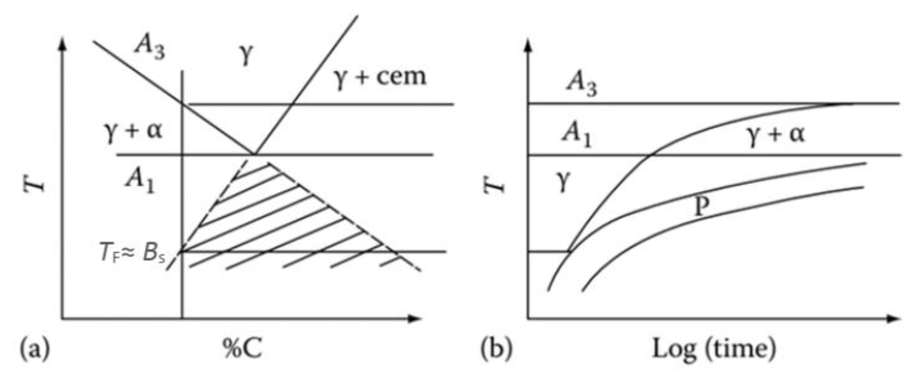
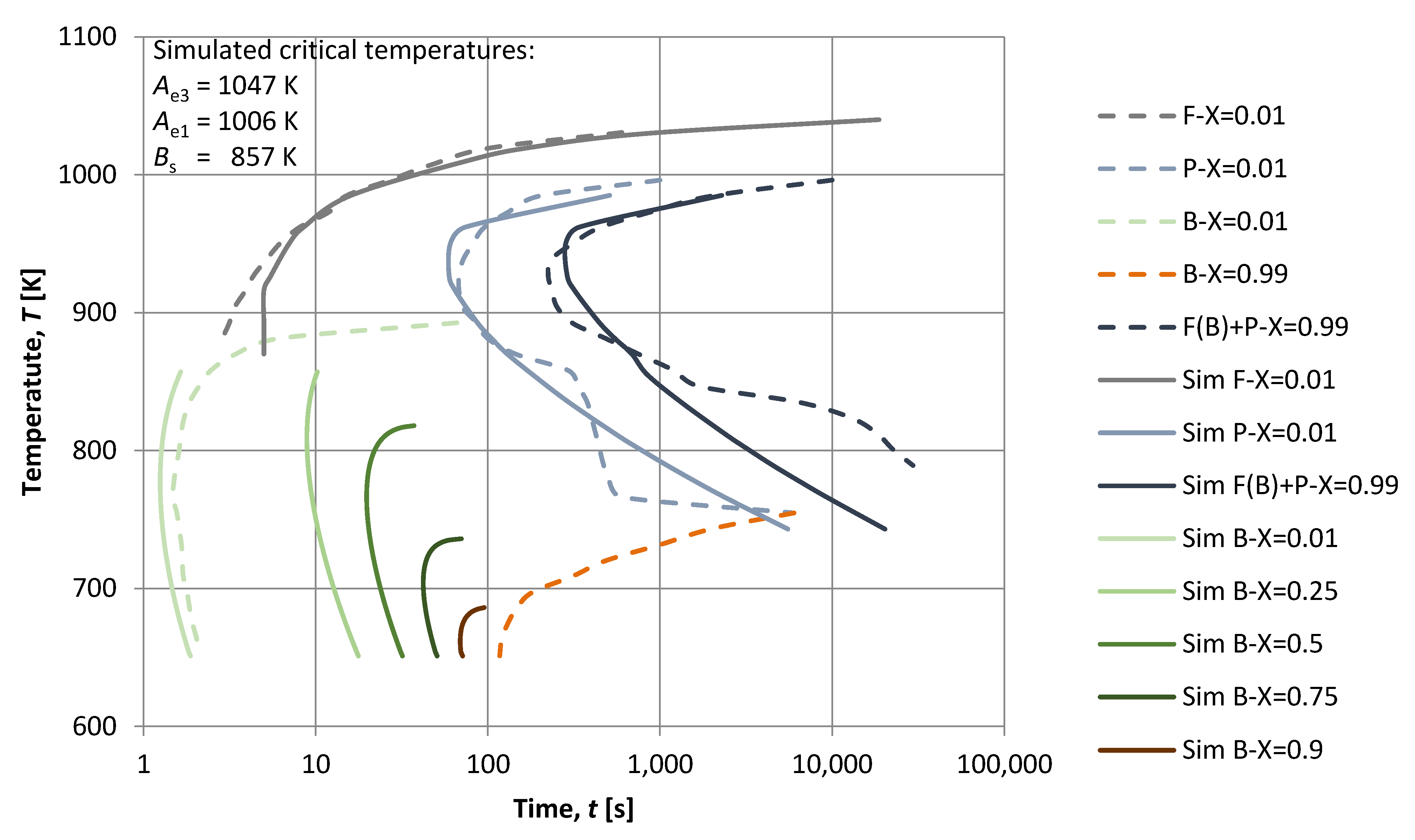
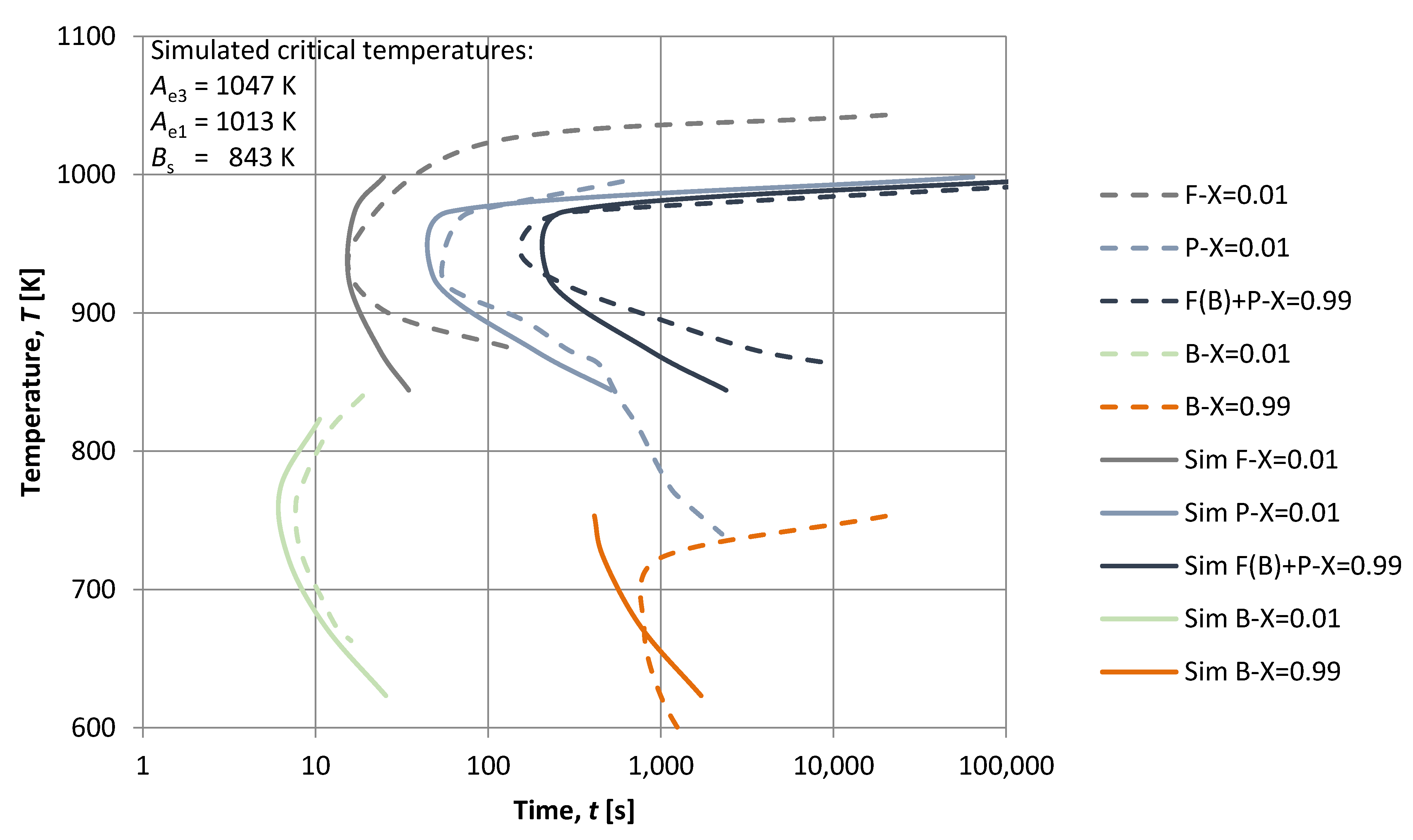
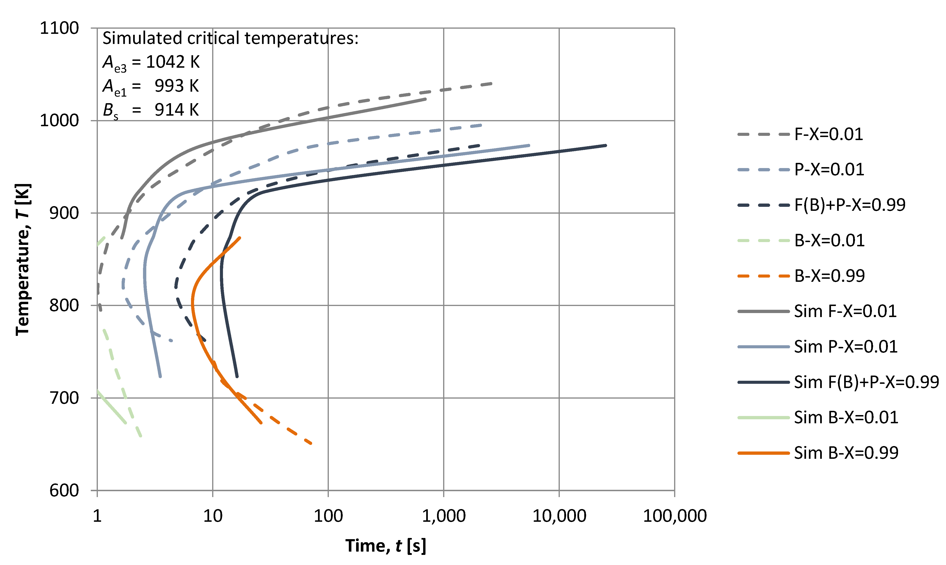
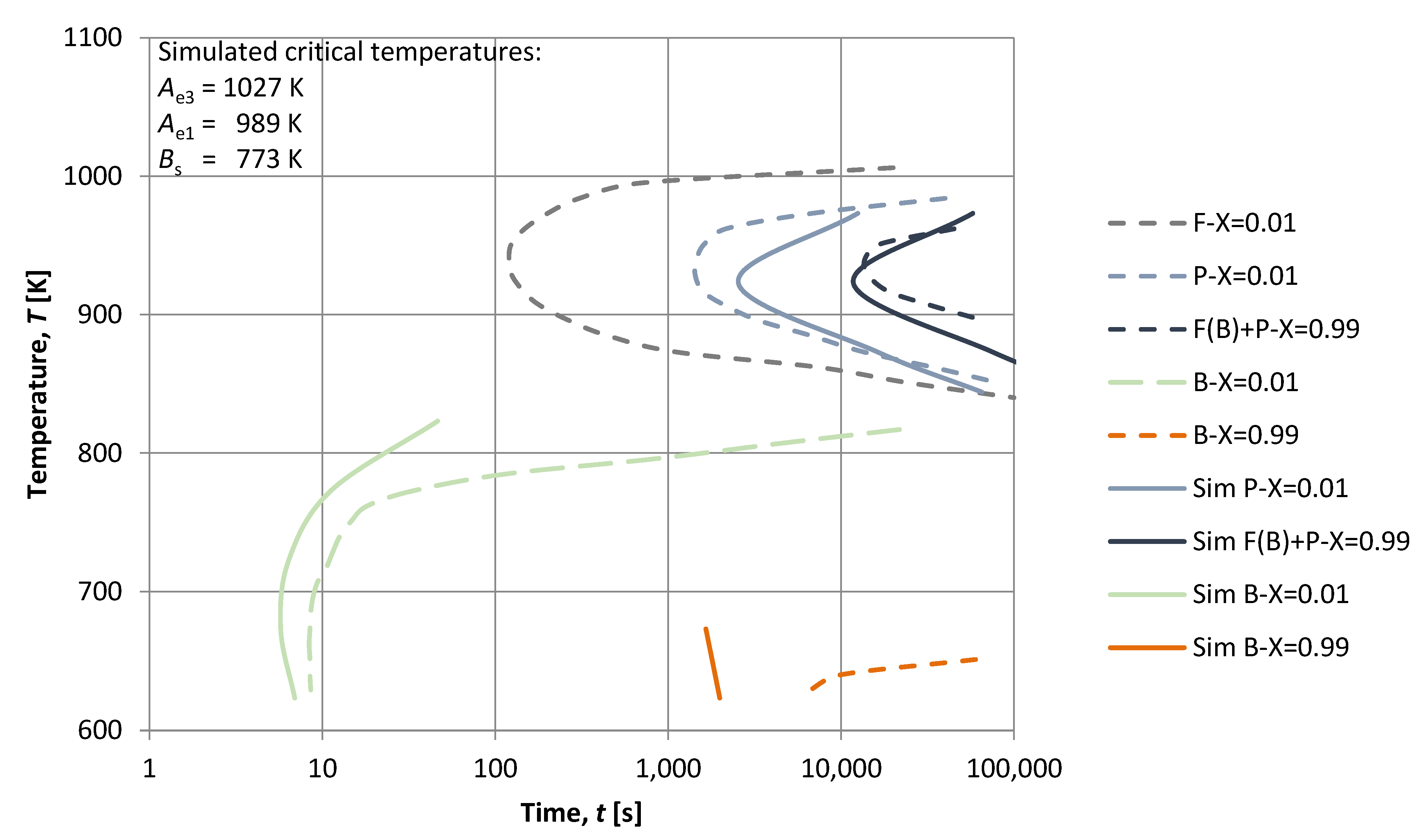
3. Results
4. Discussion
5. Conclusions
Author Contributions
Funding
Data Availability Statement
Acknowledgments
Conflicts of Interest
References
- Pan, J.; Gu, J.; Zhang, W. Industrial Applications of Computer Simulation of Heat Treatment and Chemical Heat Treatment. In Handbook of Thermal Process Modeling of Steels; Gür, C.H., Pan, J., Eds.; CRC Press: Boca Raton, FL, USA, 2009; pp. 673–701. [Google Scholar]
- Reti, T.; Felde, I.; Guerrero, M.; Sarmiento, S. Using generalized time-temperature parameters for predicting the hardness change occurring during tempering. In Proceedings of the International Conference on New Challenges in Heat Treatment and Surface Engineering, Dubrovnik–Cavtat, Dubrovnik, Croatia, 9–12 June 2009; Smoljan, B., Matijević, B., Eds.; Listemann AG: Bendern, Switzerland, 2009; pp. 333–342. [Google Scholar]
- Smokvina Hanza, S. Mathematical Modeling and Computer Simulation of Microstructure Transformations and Mechanical Properties During Steel Quenching. Ph.D. Thesis, University of Rijeka, Rijeka, Croatia, 2011. (In Croatian). [Google Scholar]
- Smoljan, B.; Iljkić, D.; Totten, G. Mathematical modeling and simulation of hardness of quenched and tempered steel. Met. Mater. Trans. B 2015, 46, 2666–2673. [Google Scholar] [CrossRef]
- Rose, A.; Wever, F. Atlas zur Wärmebehandlung der Stähle I; Verlag Stahleisen: Düsseldorf, Germany, 1954. [Google Scholar]
- Hillert, M. Discussion of “a personal commentary on transformation of austenite at constant subcritical temperatures”. Metall. Mater. Trans. A 2011, 42, 541–542. [Google Scholar] [CrossRef]
- Zener, C. Kinetics of decomposition of austenite. Trans. AIME 1946, 167, 550–595. [Google Scholar]
- Zener, C. Theory of growth of spherical precipitates from solid solution. J. Appl. Phys. 1949, 20, 950–953. [Google Scholar] [CrossRef]
- Serajzadeh, S. A mathematical model for prediction of austenite phase transformation. Mater. Lett. 2004, 58, 1597–1601. [Google Scholar] [CrossRef]
- Militzer, M.; Hawbolt, E.B.; Meadowcroft, T.R. Microstructural model for hot strip rolling of high-strength low-alloy steels. Met. Mater. Trans. A 2000, 31, 1247–1259. [Google Scholar] [CrossRef]
- Avrami, M. Kinetics of phase change. I general theory. J. Chem. Phys. 1939, 7, 1103–1112. [Google Scholar] [CrossRef]
- Simsir, C.; Gür, C.H. Simulation of quenching. In Handbook of Thermal Process Modeling of Steels; Gür, C.H., Pan, J., Eds.; CRC Press: Boca Raton, FL, USA, 2009; pp. 341–425. [Google Scholar]
- Christian, J.W. The Theory of Transformations in Metals and Alloys, 1st ed.; Pergamon Press: Oxford, UK, 2002. [Google Scholar]
- Suehiro, M. A mathematical model for predicting temperature of steel during cooling based on microstructural evolution. In Proceedings of the 11th Congress of IFHTSE and 4th ASM Heat Treatment and Surface Engineering Conference in Europe, Florence, Italy, 19–21 October 1998; Volume 1, pp. 11–20. [Google Scholar]
- Offerman, S.; van Wilderen, L.; van Dijk, N.; Sietsma, J.; Rekveldt, M.; van der Zwaag, S. In-situ study of pearlite nucleation and growth during isothermal austenite decomposition in nearly eutectoid steel. Acta Mater. 2003, 51, 3927–3938. [Google Scholar] [CrossRef]
- Whiting, M. A reappraisal of kinetic data for the growth of pearlite in high purity Fe-C eutectoid alloys. Scr. Mater. 2000, 43, 969–975. [Google Scholar] [CrossRef]
- Davenport, E.S.; Bain, E.C. Transformation of austenite at constant subcritical temperatures. Trans. Met. Soc. AIME 1930, 90, 117–154. [Google Scholar]
- Bhadeshia, H.K.D.H. Bainite in Steels: Transformations, Microstructure and Properties, 2nd ed.; IOM Communications: London, UK, 2001. [Google Scholar]
- Fielding, L.C.D. The bainite controversy. Mater. Sci. Technol. 2013, 29, 383–399. [Google Scholar] [CrossRef]
- Yang, Z.-G.; Fang, H.-S. An overview on bainite formation in steels. Curr. Opin. Solid State Mater. Sci. 2005, 9, 277–286. [Google Scholar] [CrossRef]
- Hillert, M. The nature of bainite. ISIJ Int. 1995, 35, 1134–1140. [Google Scholar] [CrossRef]
- Quidort, D.; Bréchet, Y.J.M. A model of isothermal and non isothermal transformation kinetics of bainite in 0.5% C steels. ISIJ Int. 2002, 42, 1010–1017. [Google Scholar] [CrossRef]
- Rees, G.I.; Bhadeshia, H.K.D.H. Bainite transformation kinetics part 1 modified model. Mater. Sci. Technol. 1992, 8, 985–993. [Google Scholar] [CrossRef]
- Pan, Y.-T. Measurement and Modelling of Diffusional Transformation of Austenite in C.-Mn Steels. Ph.D. Thesis, Institute of Materials Science and Engineering of the National Sun Yat-Sen University, Kaohsiung, Taiwan, 2001. [Google Scholar]
- Rose, A.; Hougardy, H. Atlas zur Wärmebehandlung der Stähle; Verlag Stahleisen: Düsseldorf, Germany, 1972. [Google Scholar]
- Lusk, M.T.; Lee, Y.-K. A global material model for simulating the transformation kinetics of low alloy steels. In Proceedings of the 7th International Seminar of IFHT: Heat Treatment and Surface Engineering of Light Alloys, Budapest, Hungary, 15–17 September 1999; Lendvai, J., Réti, T., Eds.; Hungarian Scientific Society of Mechanical Engineering: Budapest, Hungary, 1999; pp. 273–282. [Google Scholar]
- Steven, W.; Haynes, A.G. The temperature of formation of martensite and bainite in low alloy steels. J. Iron Steel Inst. 1956, 183, 349–359. [Google Scholar]


| Designation (DIN) | Chemical Composition, wt. % | |||||||||
|---|---|---|---|---|---|---|---|---|---|---|
| C | Si | Mn | P | S | Cr | Cu | Mo | Ni | V | |
| 42CrMo4 | 0.38 | 0.23 | 0.64 | 0.019 | 0.013 | 0.99 | 0.17 | 0.16 | 0.08 | <0.01 |
| Ck45 | 0.44 | 0.22 | 0.66 | 0.022 | 0.029 | 0.15 | - | - | - | 0.02 |
| 28NiCrMo74 | 0.30 | 0.24 | 0.46 | 0.030 | 0.025 | 1.44 | 0.20 | 0.37 | 2.06 | <0.01 |
| 34Cr4 | 0.35 | 0.23 | 0.65 | 0.026 | 0.013 | 1.11 | 0.18 | 0.05 | 0.23 | <0.01 |
| 25CrMo4 | 0.22 | 0.25 | 0.64 | 0.010 | 0.011 | 0.97 | 0.16 | 0.23 | 0.33 | <0.01 |
| 36Cr6 | 0.36 | 0.25 | 0.49 | 0.021 | 0.020 | 1.54 | 0.16 | 0.03 | 0.21 | <0.01 |
| 41Cr4 | 0.44 | 0.22 | 0.80 | 0.030 | 0.023 | 1.04 | 0.17 | 0.04 | 0.26 | <0.01 |
| Transformation | Constant | Steel Designation (DIN) | ||||||
|---|---|---|---|---|---|---|---|---|
| 42CrMo4 | Ck45 | 28NiCrMo74 | 34Cr4 | 25CrMo4 | 36Cr6 | 41Cr4 | ||
| Ferrite | k1 | 2.5 × 10⁵ | 2.5 × 10⁵ | - | 2.5 × 10⁵ | 2.5 × 10⁵ | 2.5 × 10⁵ | 2.5 × 10⁵ |
| k2 | 3.8321 × 10⁻⁵ | 1.7441 × 10⁻⁴ | - | 9.0625 × 10⁻¹⁰ | 6.3183 × 10⁻⁸ | 8.8213 × 10⁻⁹ | 1.1941 × 10⁻⁹ | |
| n1 | 4.6923 | 5.2095 | - | 2.3955 | 3.3200 | 2.5230 | 2.3547 | |
| a1 | 8.8839 | 8.7592 | - | 7.8504 | 3.1064 | 10.0511 | 14.7870 | |
| a2 | −0.0115 | −0.0114 | - | −0.0101 | −0.0039 | −0.0130 | −0.0195 | |
| a3 | −1.8688 | −4.4695 | - | −1.7667 | −1.4606 | −1.5163 | −1.7387 | |
| a4 | 0.0032 | 0.0070 | - | 0.0030 | 0.0024 | 0.0027 | 0.0031 | |
| Pearlite | k3 | 27,988,177 | 76,767,479 | 16,492,913 | 31,355,038 | 43,316,272 | 56,142,707 | 93,514,410 |
| k4 | 1.1450 × 10⁻¹¹ | 9.8057 × 10⁻⁵ | 2.1918 × 10⁻¹⁹ | 6.1325 × 10⁻¹² | 8.6385 × 10⁻¹⁷ | 2.5088 × 10⁻¹⁷ | 5.4094 × 10⁻¹² | |
| k5 | 51,728 | −92,146 | 214,273 | 47,324 | 149,610 | 151,595 | 46,211 | |
| Bainite | k6 | −99,033 | 51128 | −101,946 | −15,089 | −77,442 | −34,123 | −16,704 |
| k7 | 3.2308 × 10⁸ | 2.4803 × 10⁹ | 2.0943 × 10⁹ | 2.5027 × 10⁹ | 2.5966 × 10⁶ | 2.2482 × 10⁹ | 1.6819 × 10⁹ | |
| k8 | 5.4488 × 10⁷ | 1.1746 × 10²⁰ | 8.1265 × 10⁷ | 8.0362 × 10¹⁴ | 6.6340 × 10¹⁰ | 2.7482 × 10¹² | 4.2311 × 10¹³ | |
| nB | 1.4923 | 2.30043 | 1.09856 | 1.58602 | 1.12141 | 1.51777 | 1.74637 | |
| a5 | 2.989028 | 1.000000 | - | 2.349733 | 2.794667 | 3.587317 | 2.881892 | |
| a6 | −0.003041 | 0.00000 | - | −0.002139 | −0.002667 | −0.003902 | −0.002973 | |
| Quantity Value | Units | Description |
|---|---|---|
| D0 = 2.3 × 10⁻⁵ | m2 s−1 | Material constant |
| Qdif = 1.48 × 10⁵ | J mol−1 | Diffusion activation energy |
| R = 8.314 | J mol−1 K−1 | Universal gas constant |
| S = 170153 | m−1 | Surface of austenite grain suitable for nucleation |
| cγ = 1186.661 exp(−7.2834 × 10⁻³ T) | wt.% C | Concentration of austenite |
| cα = 0.1592−1.3423 × 10⁻⁴ T | wt.% C | Concentration of ferrite |
| cγα = 9.6782−8.82 × 10⁻³ T | wt.% C | Concentration of austenite at the boundary with ferrite |
| cγFe3C = −0.5248 + 1.28 × 10⁻³ T | wt.% C | Concentration of austenite at the boundary with cementite |
Publisher’s Note: MDPI stays neutral with regard to jurisdictional claims in published maps and institutional affiliations. |
© 2021 by the authors. Licensee MDPI, Basel, Switzerland. This article is an open access article distributed under the terms and conditions of the Creative Commons Attribution (CC BY) license (https://creativecommons.org/licenses/by/4.0/).
Share and Cite
Smoljan, B.; Iljkić, D.; Smokvina Hanza, S.; Hajdek, K. Mathematical Modelling of Isothermal Decomposition of Austenite in Steel. Metals 2021, 11, 1292. https://doi.org/10.3390/met11081292
Smoljan B, Iljkić D, Smokvina Hanza S, Hajdek K. Mathematical Modelling of Isothermal Decomposition of Austenite in Steel. Metals. 2021; 11(8):1292. https://doi.org/10.3390/met11081292
Chicago/Turabian StyleSmoljan, Božo, Dario Iljkić, Sunčana Smokvina Hanza, and Krunoslav Hajdek. 2021. "Mathematical Modelling of Isothermal Decomposition of Austenite in Steel" Metals 11, no. 8: 1292. https://doi.org/10.3390/met11081292
APA StyleSmoljan, B., Iljkić, D., Smokvina Hanza, S., & Hajdek, K. (2021). Mathematical Modelling of Isothermal Decomposition of Austenite in Steel. Metals, 11(8), 1292. https://doi.org/10.3390/met11081292