Modeling of Isothermal Dissolution of Precipitates in a 6061 Aluminum Alloy Sheet during Solution Heat Treatment

Abstract

During the solution heat treatment (SHT) process of aluminum alloys, precipitates dissolve into the matrix. To predict the dissolution time, modeling of isothermal dissolution of precipitates in 6061 aluminum alloy during SHT was conducted. A precipitate dissolution model was established, and the flowchart of the modeling was designed as well. Then the explicit finite-difference method was employed to solve the dissolution model, and the mobile nodes method was used to deal with the moving interface. The simulation was based on real precipitates in 6061, and SHT experiments were conducted to validate the numerical model. The simulation results showed that the isothermal dissolution time of precipitates in 6061-T6 aluminum alloy at 560 °C is 11.6856 s. The dissolution time in the simulation was close to the experimental results, with an error of 16.7%, indicating that the modeling in this study was fairly reasonable and accurate. The error was caused by many factors, and the model should be improved.

1. Introduction

The aluminum alloy 6061 is a precipitated hardening alloy containing magnesium (Mg) and silicon (Si) as its chief alloying elements, and thus it is a heat-treated alloy [1]. Benefitting from a high specific strength, good impact energy absorption, high corrosion resistance, superior weldability and castability, 6061 aluminum alloy is used for various engineering and structural components [1,2,3,4]. This alloy is the most versatile alloy used in the construction of marine fittings, yachts, chassis, bearing and scuba tanks, ships, and transport components, along with aircraft structure and automobile components [1,5,6]. The alloy can be shaped by extrusion [7], forging [8], casting [1], stamping [5], additive manufacturing [9], etc. In these forming processes, as a kind of heat-treated alloy, 6061 aluminum alloy usually undergoes a series of heat treatment processes, including solution heat treatment (SHT), quenching, and aging. During the SHT process, the nanoscale precipitates dissolve into the matrix. Usually, a quenching process is carried out after SHT and then an alternative aging process is conducted to improve the strength. Therefore, this alloy is mostly available in different designations, such as annealed, pre-tempered 6061-O; solution-heat-treated and naturally aged 6061-T4; and solution-heat-treated and artificially aged 6061-T6 [1]. The alloy 6061-T6 is more commonly used [1] because it has higher strength than 6061-O and 6061-T4 alloys. SHT and artificial aging processes are needed to achieve high strength. However, SHT usually takes a considerably longer time than 10 min [10] and thus it is inefficient. As a consequence, it is necessary to optimize or improve the SHT process to reduce the SHT time. Numerical simulation is a method that makes it possible to predict the dissolution time of precipitates by appropriate kinetic theory [11] and thus to optimize the SHT process with reduced cost and fewer experiments.

Whelan deduced the formula for the dissolution of a single spherical precipitate in an infinite space without considering the effect of dissolution of other precipitated phases on solute diffusion [12], and therefore the dissolution time was less [13]. Cheng et al. [14] derived the steady and transient components of the dissolution rate. By combining the model with the Johnson–Mehl–Avrami (JMA) type equation, the dissolution rates of precipitates considering the interaction of adjacent precipitates was obtained by Zuo et al. [15], and the accuracy was verified in Al–Cu and Al–Si alloys. Employing the model in [15], Zhang et al. [11] calculated the dissolution time of an Al–Mg–Si–Cu alloy. Experiments showed that it took 15 s at 555 °C for the precipitated phase to dissolve, and the dissolution time was also related to the size of the precipitated phase. However, this model does not properly indicate the influence of different alloying elements on the dissolution process. In fact, the results obtained above are calculated by derived empirical formulas. Vermolen et al. have done a lot of work in the numerical simulation of the second-phase dissolution, including one-dimensional [16] and three-dimensional [17] simulations in binary alloys and dissolution simulation of the second phase in ternary alloys [18,19]. Then Chen et al. [20] carried out a differential scanning caborimetry (DSC)experimental study of the dissolution kinetics of β precipitates in an Al–Mg–Si alloy to test the validity of the particle dissolution model in [18,19], and the results demonstrated that the model is successful in simulating particle dissolution during linear heating. Tang et al. [21] used Computer Coupling of Phase Diagrams and Thermochemistry (CALPHAD) and diffusion-controlled transformation (DICTRA), a function in thermo-calc, to calculate the non-isothermal dissolution process of Mg₂Si in AA6063 aluminum alloy.

Simulations of microstructure evolution are expected to be based on the real microstructure of the alloy, and experiments should be performed to evaluate the accuracy of the simulation results. In this study, modeling of the isothermal dissolution of precipitates in 6061 aluminum alloy during SHT was carried out. The precipitate dissolution model was established, and a flowchart of the modeling was designed as well. Then the explicit finite-difference method was employed to solve the dissolution model, and the mobile nodes method was used to deal with the moving interface. The initial conditions of the simulation were based on real precipitates in 6061 aluminum alloy, and SHT experiments were conducted to validate the numerical model. The simulation results were also explained by the classical diffusion model. The research is anticipated to provide theoretical guidance for improving and optimizing the SHT process.

2. Models and Methods

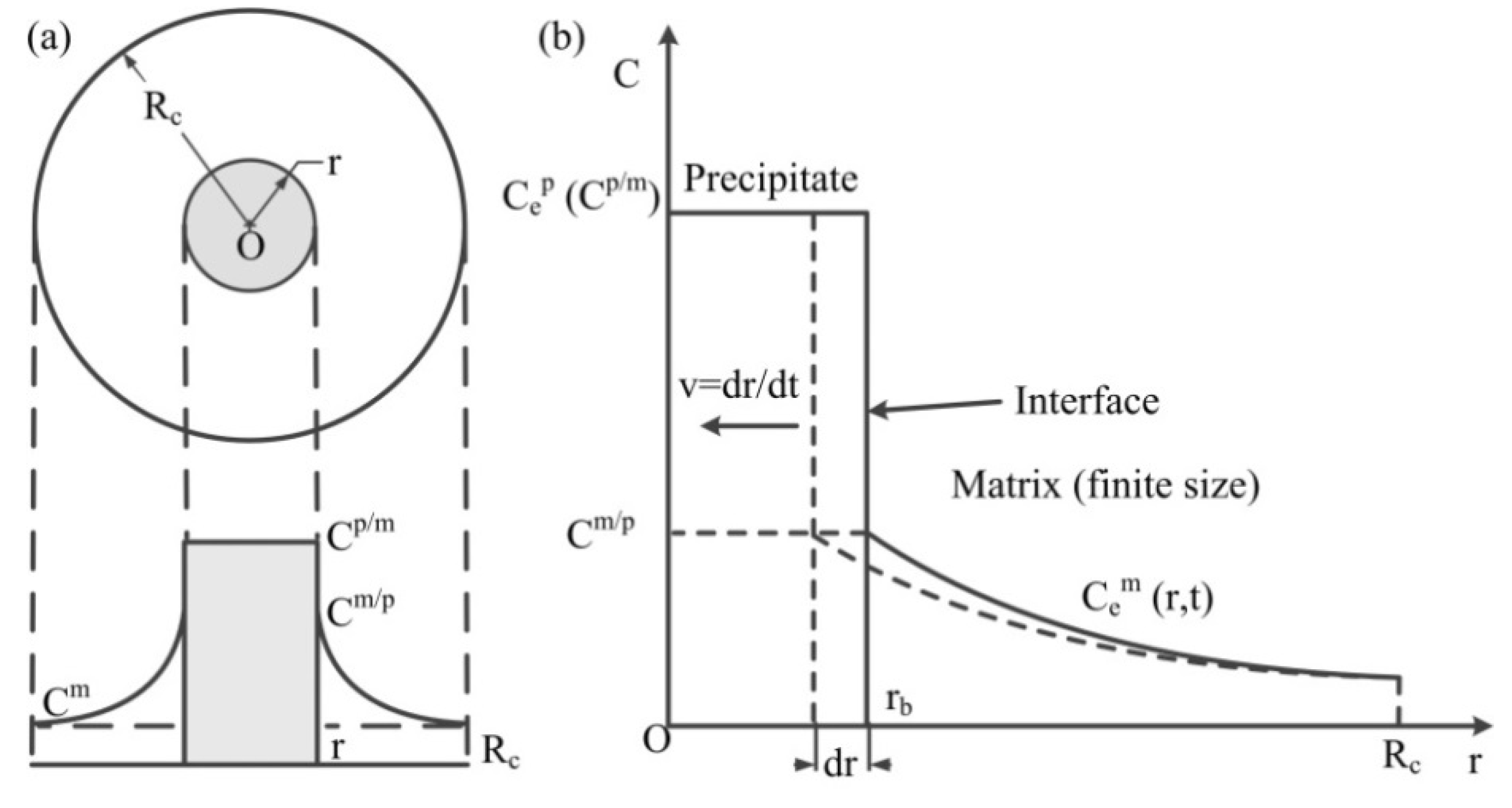
2.1. Dissolution Model

• The model was derived on the following assumptions:
• The precipitates are all spherical, with the same size, and uniformly distributed in the matrix.
• The composition and proportion of elements of the precipitates remain unchanged during the whole dissolution process.
• The solubility and diffusion coefficient of each element are not affected by other elements, concentration, and distance.
• All the precipitates are located within the grains, regardless of the dissolution of the precipitates at the grain boundary and the diffusion across the grain boundary.
• The dissolution process is isothermal.
• The precipitate dissolves in a spherical space, and there is only one precipitate in this space.

Decomposition of the precipitates and crossing of alloying elements through the interface between the precipitates and the matrix are referred to as the interface reactions or the interface-controlled mechanism [22]. The two processes are sufficiently fast compared with the long-distance diffusion of the alloying elements in the matrix [22], and thus the decomposition time of precipitates and the crossing time of alloying elements through the interface can be ignored.

As shown in Figure 1a, the precipitate with a radius r (initial radius is r₀) is in a spherical space with a radius Rc. As assumed, the spherical space with a radius Rc is the space where the precipitate dissolves and Rc meets Equation (1). The shape of the diffusion field a distance away from the particle was considered to be approximately spherical, even for a thin-disc-like precipitate [20]. Therefore, it was reasonable to use a spherical space as a region for the calculation of alloying elements’ diffusion in the matrix. The spherical space is an independent system that does not transfer the matter to the outside.

$${\left(r_0/R\mathrm{c}\right)}^3=f_p$$

(1)

where f_p is the volume fraction of precipitates in the alloy and can be calculated by the mass fraction of precipitates in the alloy.

Figure 1b shows the interface movement under diffusion control during the dissolution of the precipitates. The alloying elements are denoted by e, and for 6061, e = Mg, Si, or Al. $C^{p/m}$ denotes the mass concentration (wt%; the concentrations following all refer to the mass concentration) on the precipitate side at the precipitate–matrix interface and equals $C_e^p$, which means the concentration of the alloying element e in precipitates. $C_e^m$ denotes the concentration of the alloying element e in the matrix, and it varies with the position r and the time t. $C_{}^{m/p}$ denotes the concentration on the matrix side at the precipitate–matrix interface (r_b denotes the position of the interface) and equals $C_e^m$(r = r_b, t).

As indicated in Figure 1b, the position of the interface (r, spherical surface) is r_b before moving; then the interface moves a small distance of dr in a short time dt. So the total amount of atoms for the alloying element e gathering at the interface is

$$A_e=(C_e^p\frac{{\rho }^p}{M_e}-C_e^{m/p}\frac{{\rho }^m}{M_e})4\pi r^{2}dr$$

(2)

where ${\rho }^p$, ${\rho }^m$, and $M_e$ are the density of the precipitate (kg/m³), the density of the matrix (kg/m³), and the molar mass (kg/mol) of the alloying element e, respectively. According to Fick′s first law, the total amount of atoms of the alloying element e gathering at the interface can also be expressed as

$$A_e=\left((-D_e^p\frac{\partial C_e^p}{\partial r}{|}_{r=r_b})\frac{{\rho }^{\mathrm{e}}}{M_e}-(-D_e^m\frac{\partial C_e^m}{\partial r}{|}_{r=r_b})\frac{{\rho }^m}{M_e}\right)4\pi r^{2}dt$$

(3)

where $D_e^p$ and $D_e^m$ (m²/s) denote the diffusion coefficients in the precipitate and the matrix, respectively. In Equation (3), the concentration gradient in the precipitate is zero, and thus the moving velocity of the interface, namely the dissolution rate, is

$$v=\frac{dr}{dt}=\frac{D_e^m\frac{\partial C_e^m}{\partial r}{|}_{r=r_b}}{C_e^p\frac{{\rho }^p}{{\rho }^m}-C_e^{m/p}}$$

(4)

The diffusion coefficient is related to the temperature [23]:

$$D_e^m=D_{{}_0}^e\exp \left(\frac{-Q_{\mathrm{e}}}{RT}\right)$$

(5)

where $D_{{}_0}^e$ (m²/s) and Q_e (J/mol) are the diffusion parameter and the thermal diffusion activation energy of the alloying element e, respectively, and T (K) is the Kelvin temperature.

The dissolution rates of the different elements should be equal, which means that

$$\frac{D_{Mg}^m\frac{\partial C_{Mg}^m}{\partial r}{|}_{r=r_b}}{C_{Mg}^p\frac{{\rho }^p}{{\rho }^m}-C_{Mg}^{m/p}}=\frac{D_{Si}^m\frac{\partial C_{Si}^m}{\partial r}{|}_{r=r_b}}{C_{Si}^p\frac{{\rho }^p}{{\rho }^m}-C_{Si}^{m/p}}$$

(6)

To simplify the model, the precipitates in 6061 aluminum alloy were thought to be Mg₂Si, and thus the concentration of each element on the matrix side at the interface satisfied the local equilibrium [23]:

$$(C_{Mg}^{m/p}{)}^{\frac{2}{3}}(C_{Si}^{m/p}{)}^{\frac{1}{3}}=K_0\exp (\frac{-Q_{Al}}{RT})$$

(7)

where Q_Al (J/mol) is the activation energy of Al and K₀ (wt. %) is the solubility product parameter.

The diffusion of each element in the matrix follows Fick′s second law (the one-dimensional diffusion based on a spherical coordinate system was used in this study):

$$\frac{\partial C_e^m}{\partial t}=\frac{D_e^m}{r^2}\frac{\partial }{\partial r}(r^2\frac{\partial C_e^m}{\partial r})$$

(8)

The boundary conditions were as follows: there is no inflow or outflow of solute atoms at the spherical space boundary (Neumann boundary condition), namely Equation (9), and no solute atoms flow into or out of the spherical core after the dissolution of the precipitate (Neumann boundary condition), namely Equation (10).

$$\frac{\partial C_e^m}{\partial r}{|}_{r=R_{\mathrm{c}}}=0$$

(9)

$$\frac{\partial C_e^m}{\partial r}{|}_{r=0}=0$$

(10)

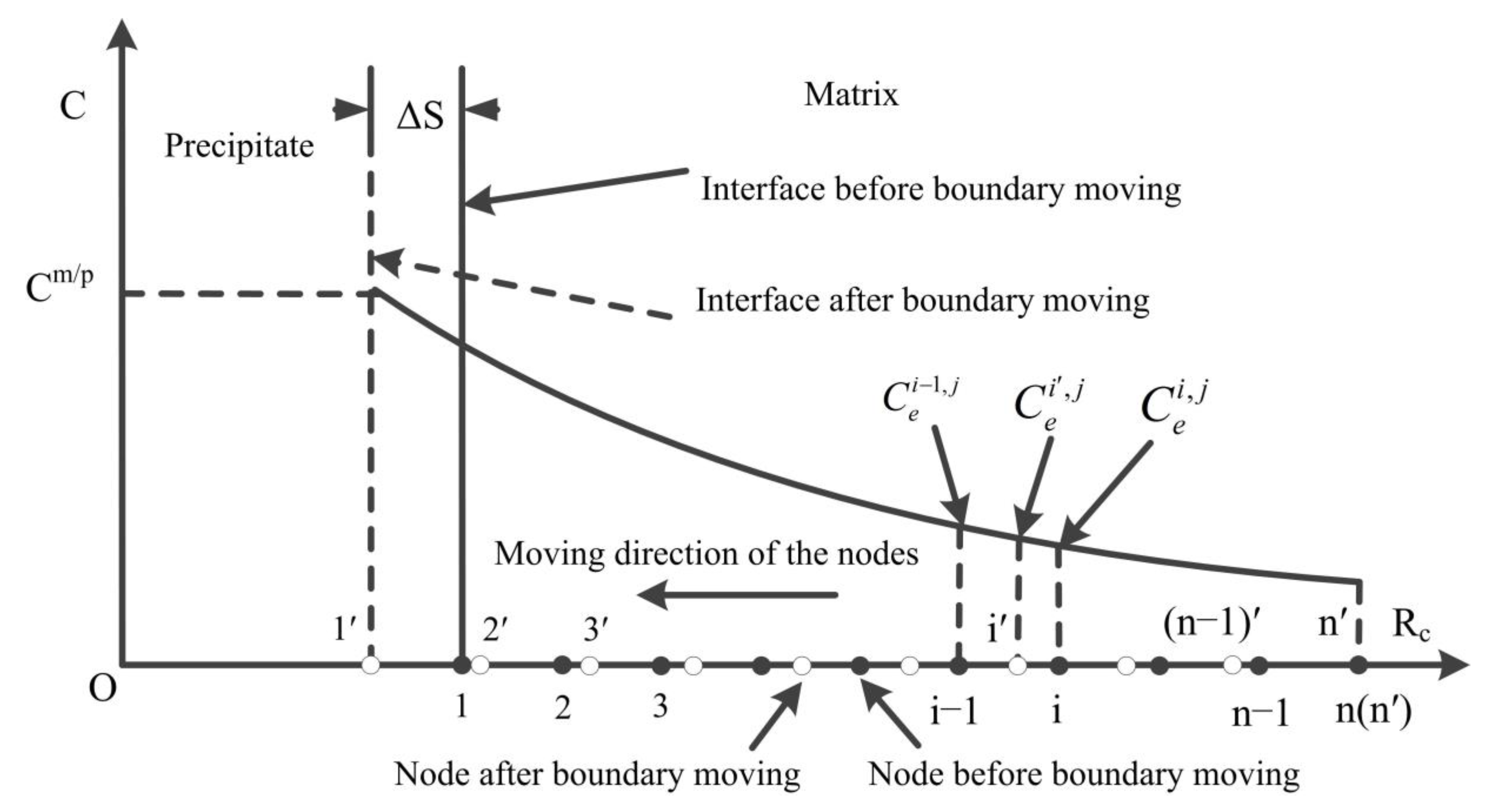
2.2. Model Discretization and Mobile Nodes Method

The explicit finite-difference method was adopted to solve the above model. The time step was constant during the calculation process, and the space step (node space) of the same time step was the same. The forward difference was used for the first-order difference, and the central difference was used for the second-order difference. Therefore, the calculation results were accurate in the first order. With this discretization method, Equation (8) can be expressed as

$$\begin{array}{l}{C}_e^{i,j+1}=\{\frac{D_e^m\Delta t}{(\Delta r^j{)}^2}+\frac{2D_e^m\Delta t}{\left[r^j+(i-1)\Delta r^j\right]\Delta r^j}\}{C}_e^{i+1,j}+\frac{D_e^m\Delta t}{(\Delta r^j{)}^2}{C}_e^{i-1,j}\\ +\{1-\frac{2D_e^m\Delta t}{(\Delta r^j{)}^2}-\frac{2D_e^m\Delta t}{\left[r^j+(i-1)\Delta r^j\right]\Delta r^j}\}{C}_e^{i,j}\end{array}$$

(11)

where i and j are, respectively, the node number and the time step number; $\Delta t$ denotes the time step; $\Delta r^j$ denotes the spatial step at the j-th time step; and r^j is the initial radius of the precipitate at the j-th time step, namely the radius of the precipitate after the interface moves in the previous time step. In addition, both the concentration gradient and the boundary conditions were discretized in the form of a forward difference.

Since the explicit finite-difference method was employed, to keep the stability of the solution, the following conditions need to be met:

$$1-\frac{2D_e^m\Delta t}{(\Delta r^j{)}^2}-\frac{2D_e^m\Delta t}{\left[r^j+(i-1)\Delta r^j\right]\Delta r^j}\ge 0$$

(12)

Considering that the above relevant parameters are all positive, the stability condition can be simplified to

$$\frac{D_e^m\Delta t}{(\Delta r^j{)}^2}+\frac{D_e^m\Delta t}{(r^j+\Delta r^j)\Delta r^j}\le \frac{1}{2}$$

(13)

As a result, a reasonable spatial step and time step are necessary and the judgment conditions are set in the modeling calculation program, meaning that if Equation (13) is not valid for Si or Mg, the calculation terminates.

As indicated in Figure 2, the interface moves during the dissolution process, and this means that the radius of the precipitate decreases while the size of the matrix increases. The mobile nodes method was used to deal with the moving interface. Since only the matrix was meshed, the matrix would be re-meshed after the interface moved. The total node numbers were kept unchanged, and the interface was always at the first node. The solid dot denotes the node before moving (i), and the hollow dot denotes the node after moving (i′) in Figure 2. Please note that the node position at the boundary of the spherical space was fixed. In each time step before the precipitate dissolved, the concentration at each node was calculated by Equation (11), and then the nodes were re-meshed based on the distance moved by the interface, $\Delta S^j$. Finally, the concentration of the new node could be calculated by linear interpolation:

$$C_e^{i^{\prime },j}=\frac{C_e^{i-1,j}-C_e^{i,j}}{(n-1)\Delta r^j}(n-i)\Delta S^j+C_e^{i,j}$$

(14)

Please note that i = 3~n − 1 in Equation (14) and the concentration of Node n is unchanged. The concentration of Node 1 (the location of the interface) was calculated by Equations (6) and (7). The concentration of Node 2 after the interface moved was calculated by linear interpolation between Nodes 1 and 2 before the interface moved.

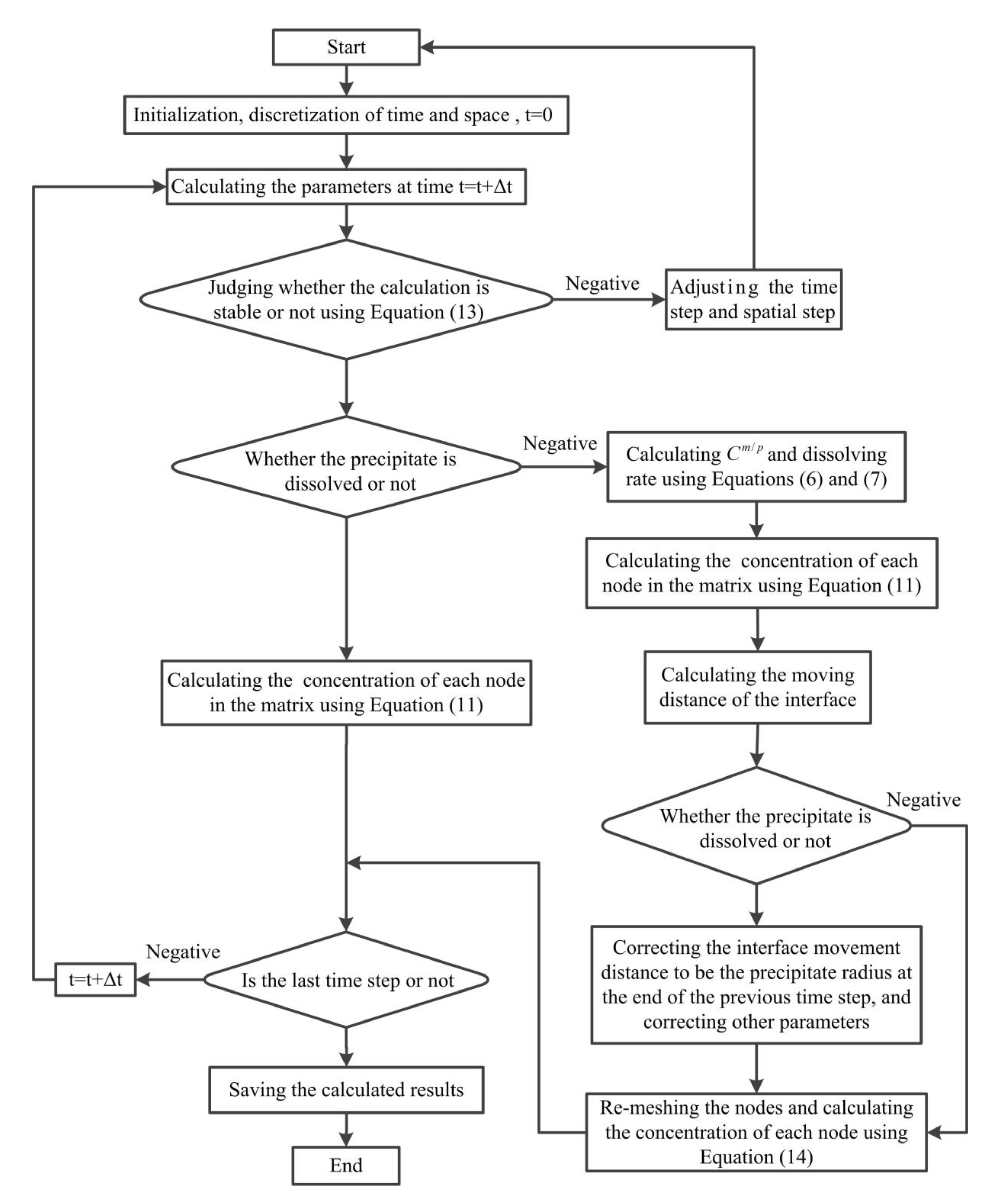
2.3. Calculation Process

The calculation process is illustrated in Figure 3. The concentration of Mg and Si on the matrix side of the interface could be obtained by Equations (6) and (7). In fact, the two equations can be converted into a cubic equation of one variable, and thus the solutions of the cubic equation can be obtained by the formula of roots or solving symbolic equations with software. Two imaginary roots were abandoned, and only one real root was adopted. As a result, the analytical solution was obtained and the iterative computations for solving the equations were avoided, saving more calculating time and guaranteeing the accuracy of the solution. This was named the direct calculation method in this study, which is also a feature of this method.

3. Simulations and Experiments

3.1. Simulation Parameters

A 6061-T6 aluminum alloy sheet with a thickness of 1.6 mm was used in this investigation. The chemical compositions of the as-received alloy were detected by optical emission spectroscopy with PDA-7000 (Shimadzu, Kyoto, Japan), and

Table 1. Chemical compositions of the as-received 6061-T6 aluminum alloy (wt. %).

Mg	Si	Mn	Cu	Fe	Cr	Ni	Zn	Ti	Al
1.104	0.676	0.078	0.150	0.423	0.165	0.006	0.210	0.027	Remain

shows the chemical compositions of the material. The hardness of the as-received alloy (after rolling) was measured in the State Key Laboratory of Materials Processing and Die and Mould Technology in China with Wilson 432 SVD (Buehler, Lake Bluff, IL USA) according to the Chinese standard GB/T 4340.1-2009. The loading force was 1 kg, and the holding time was 15 s. For each sample, at least four points were tested. Then the hardness of the as-received alloy was obtained, and its value was 112 ± 4 HV1. The heat treatment process of the as-received material was unclear, so the hardness value of the as-received material was regarded as a reference. The dimensions of the precipitate that began to dissolve were required in the simulation. The precipitates in 6061 aluminum alloy dissolve at temperatures from 450 to 590 °C [10]. However, SHT is often performed at a higher temperature than 450 °C and the precipitates have already dissolved. The dissolving rate at a lower SHT temperature was really slow, and if the heating rate was fast, the change in the precipitates’ size was small when the heating temperature difference was small. Therefore, the size of precipitates at 530 °C could be used as their size at 560 °C under conduction heating. The 6061 aluminum alloy sheet was cut to samples with dimensions [24] shown in Figure 4. The sample was heated to 530 °C at a rate of 5 °C/s by a Gleeble 3500 thermomechanical simulator (Dynamic Systems Inc., Poestenkill, NY, USA) and then water-quenched. As demonstrated in [25], nanoscale Mg–Si needles and a Mg₂Si plate can be observed in a scanning electron micrograph (Zeiss Ultra Plus 55 field emission) at 10,000 times magnification. As a result, the specimen was mechanically polished and then observed by an electronic probe EPMA-8050G (Shimadzu, Kyoto, Japan).

Figure 5 shows the micrograph of the 6061-T6 sample heated by conduction heating. The black particles (circled in Figure 5) had rod-like features and preferred orientations that were parallel or perpendicular to each other. It is suggested that the precipitates in 6061 aluminum alloy are rods or needles growing in the <100> direction (i.e., β′ or β″) or platelets lying in the {100}_Al planes (i.e., β/Mg₂Si) [26]. As mentioned above, a Mg₂Si plate can be observed in a scanning electron micrograph at 10,000 times magnification [25]. Therefore, the particles were thought to be Mg₂Si. To confirm, the element content distribution in the local area was measured by spectral analysis and the results are shown in Figure 6. The results indicated that Mg and Si are the primary elements in the two black particles (circled in Figure 6a). Additionally, the mass ratio of Mg and Si was 1.03 (Figure 6b,c), indicating once again that the two black particles are Mg₂Si.

The lengths of the five precipitates in Figure 5 were measured by image recognition based on the scale. Thus, the lengths of precipitates 1~5 were 0.622, 0.776, 0.592, 0.338, and 0.930 µm, respectively. Therefore, the size of the precipitates was 0.652 ± 0.221 µm, and the largest size was 0.930 µm. As a result, the largest initial radius of the precipitates, r₀, was 0.465 µm. The mass fraction of Mg₂Si was calculated by JMatPro (Sente Software, Guildford, UK), and then the volume fraction of Mg₂Si was obtained. The mass fraction and volume fraction of Mg₂Si were 1.02% and 1.42%, respectively. Therefore, the values of Rc could be calculated by Equation (1), and they are listed in

Table 2. Parameter values used in the simulation.

Parameters	Values	Parameters	Values
r0	0.465 µm	Rc	1.92 µm
$C_{M\mathrm{g}}^m$(r0,0)	0%	$C_{Si}^m$(r0, 0)	0%
$D_{{}_0}^{M\mathrm{g}}$	0.49 × 10−4 m2 s−1 [23]	$D_{{}_0}^{S\mathrm{i}}$	2.02 × 10−4 m2 s−1 [23]
$Q_{M\mathrm{g}}$	124 × 103 J mol−1 [23]	$Q_{Si}$	136 × 103 J mol−1 [23]
K0	89% [23]	QAl	31.97 × 103 J mol−1 [23]
${\rho }^p$	1.94 × 103 kg m−3 [27]	${\rho }^m$	2.7 × 103 kg m−3

. Assuming that the mass fractions of Mg and Si in the matrix were zero at the beginning of the calculation, the values of other parameters are listed in Table 2. The time step was 0.0001 s, and the initial spatial step was 0.02 µm; thus, the number of nodes was 74. In the simulation, the process time was 100 s. In addition, to compare the computational efficiency of the direct calculation method developed in this work and an iterative calculation method, the calculation based on the iterative method was also conducted, keeping the parameters unchanged.

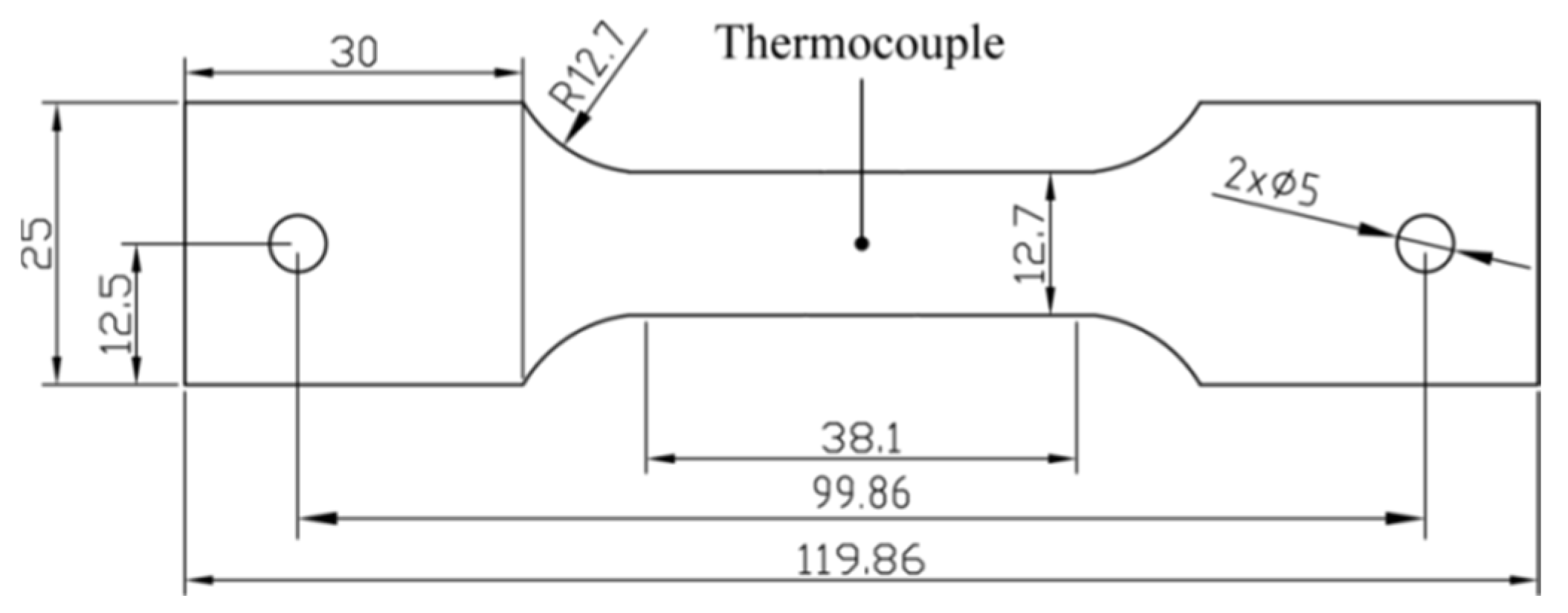
3.2. Verification Experiments

To verify the accuracy of the model and the simulations, verification experiments were carried out. Samples, as shown in Figure 4, were heated to 560 °C at a rate of 5 °C/s by a Gleeble 3500 thermomechanical simulator. Then the temperature was maintained for 3, 5, 7, 10, 13, and 15 s. After that, the samples were water-quenched and finally underwent an aging process at 200 °C for 2 h. Since the samples were conduction-heated and the ends of the samples were held by cold clamps, the temperatures of the samples were not uniform. Additionally, the thermocouple was in the middle of the samples; therefore, only the temperature in the middle of the samples was reliable. As a consequence, the Vickers hardness of each sample’s central zone was tested before and after aging.

4. Results and Discussion

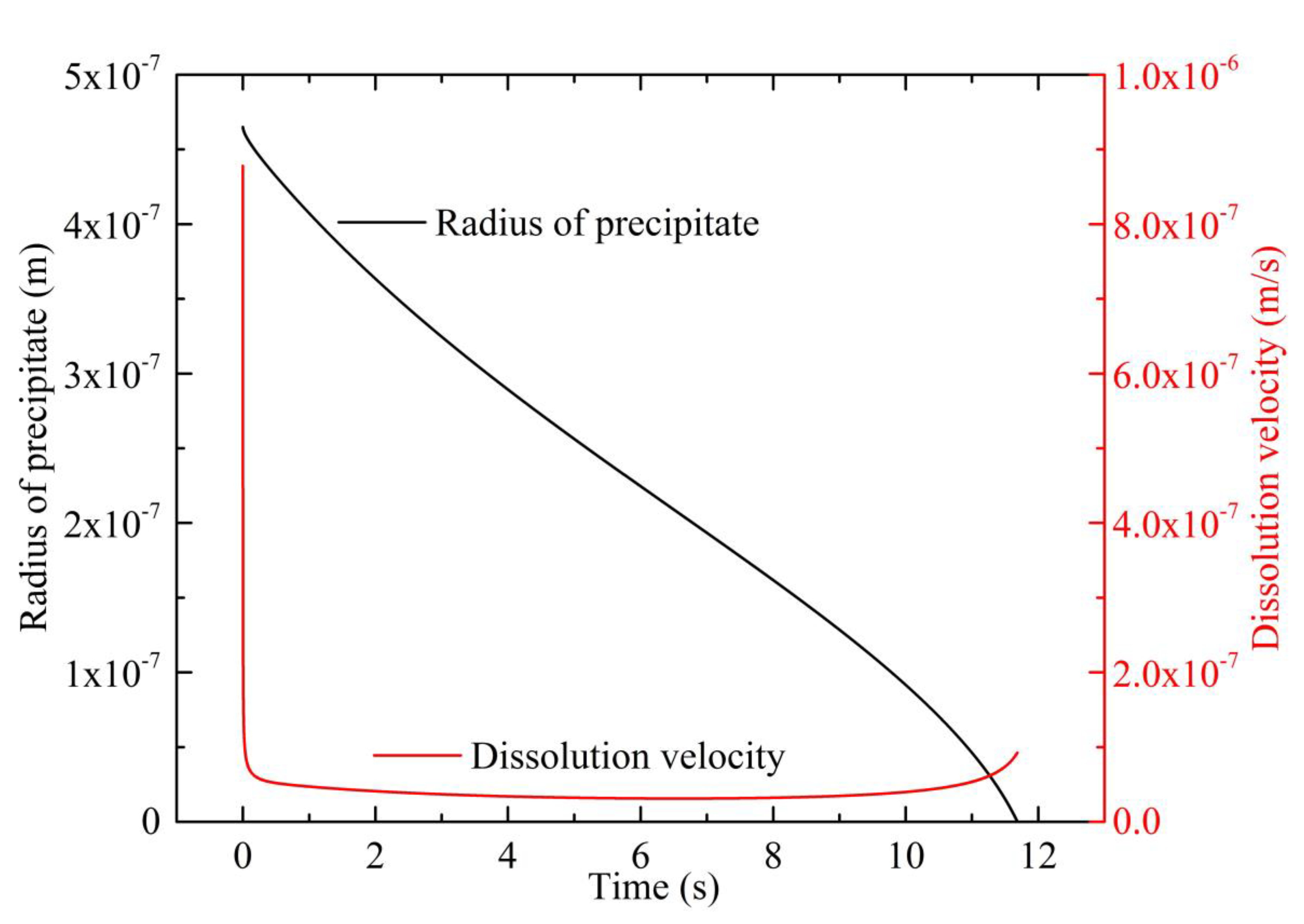
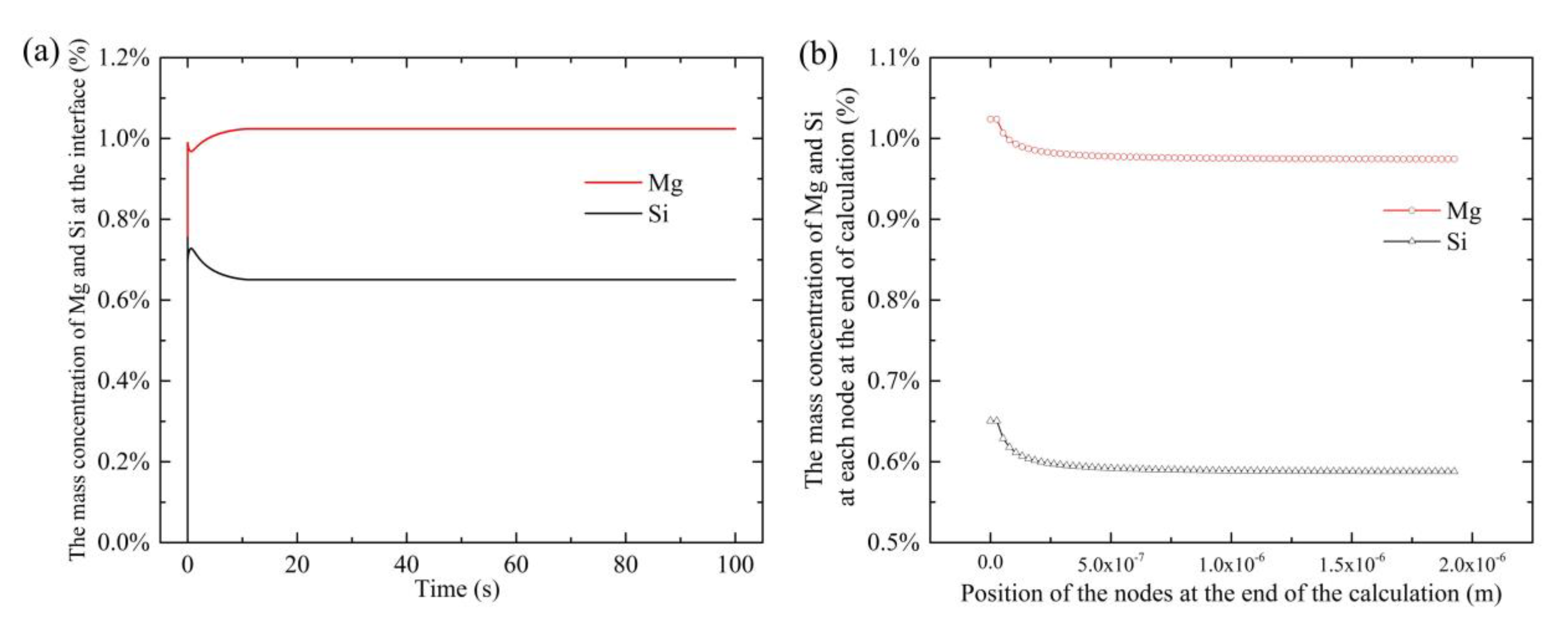
4.1. Modeling of Precipitates’ Dissolution

The total running time of the program was 123.86 s, and the completion time of dissolution was 11.6856 s. The mass errors of magnesium and silicon before and after calculation were 11.79% and 15.66%, respectively. The total running time of the calculation based on an iterative method was 1111.69 s, and the calculation time was about 9 times the time in the direct calculation method, meaning that the calculation time based on the direct calculation method reduced by about 88.9%. Though the iterative method took more time, the calculation results were the same as those of the direct calculation method. Figure 7 shows the radius of the precipitate and dissolution velocity vs. time during dissolution. The mass concentrations of Mg and Si on the boundary changed with time, as shown in Figure 8a, and the mass concentrations of nodes at the end of the calculation are shown in Figure 8b. As shown in Figure 7, the radius of the precipitate gradually decreased with increasing of time, and it was noted that the convexity–concavity of the curve changed at a specific moment: the curve was convex to the origin at the beginning and concave to the origin after a specific time point. Accordingly, the dissolving velocity decreased at first and then increased. Since the concentration gradient at the interface was large at the beginning, the dissolving velocity was large as well, as indicated by Equation (4). With the progress of dissolution, the concentration at the interface tended to be in equilibrium (Equation (7) and Figure 8a). Therefore, the concentration gradient near the interface decreased and the dissolving velocity slowly decreased. With a further increase in the dissolution time, the size of the precipitation phase decreased and the volume of the solutes’ diffusion field relatively increased. As a result, the dissolution velocity increased again. Especially, the dissolution velocity significantly increased when the precipitate was about to complete dissolution. In addition, as shown in Figure 8b, the mass concentrations of Mg and Si in the calculation region were non-uniform at the end of the calculation. This indicates that the mass concentrations were also non-uniform when the particle had just dissolved. In fact, it would take more time to homogenize the solute concentrations [28].

The change in the velocity curve can be explained by the diffusion equation. The dissolution process of a single particle in an infinite space under the control of diffusion can be expressed as [14]

$$v=\frac{(C^{m/p}-C^m)\frac{{\rho }^m}{M_m}}{C^p\frac{{\rho }^p}{M_p}-C^{m/p}\frac{{\rho }^m}{M_m}}(\frac{D^m}{r}+\sqrt{\frac{D^m}{\pi t}})$$

(15)

where $M_p$ and $M_m$ are the molar mass (kg mol⁻¹) of the precipitate and the matrix, respectively. According to Equation (15), the dissolution rate is controlled by the radius r ($D^m/r$) and the dissolution time t ($\sqrt{D^m/(\pi t)}$). At the beginning, the radius of precipitate was relatively large (non-infinite value) and the time was close to zero. Therefore, the dissolution rate was mainly controlled by $\sqrt{D^m/(\pi t)}$. As a result, the dissolution rate was large at the beginning and then decreased to a low level. In the later stage of dissolution, the radius of the precipitate became smaller (approaching zero) and the dissolution time became larger (non-infinite value). Then the dissolution rate was mainly controlled by $D^m/r$, and thus the dissolution rate increased until the dissolution process completed.

The variation trend in the precipitate radius with the solution time in Figure 7 is the same as that in literature [13,15,19]. In the works of Brown [13] and Vermolen [19], methods similar to the ones in this paper were used, and therefore it seems reasonable that the dissolution curves are similar. The difference between our work and the works of Brown [13] and Vermolen [19] is in the mobile nodes method and the direct calculation method. In Zuo’s work [15], though an approximate mathematically exact solution was used to model the secondary phase dissolution [12], similar dissolution curves of the secondary phase were obtained. However, the method in Zuo’s work [15] cannot model the dissolution of two- or three-dimensional particles.

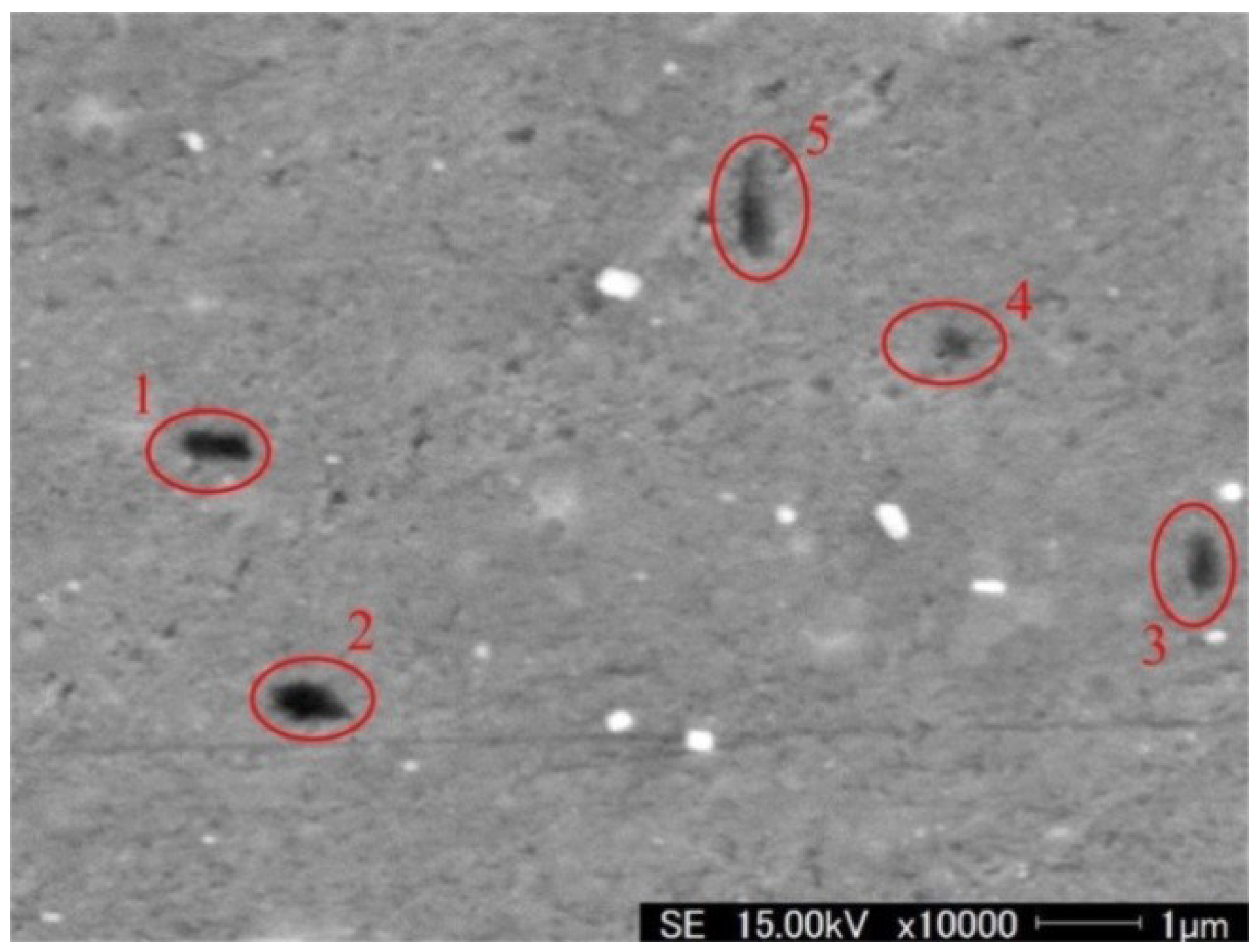
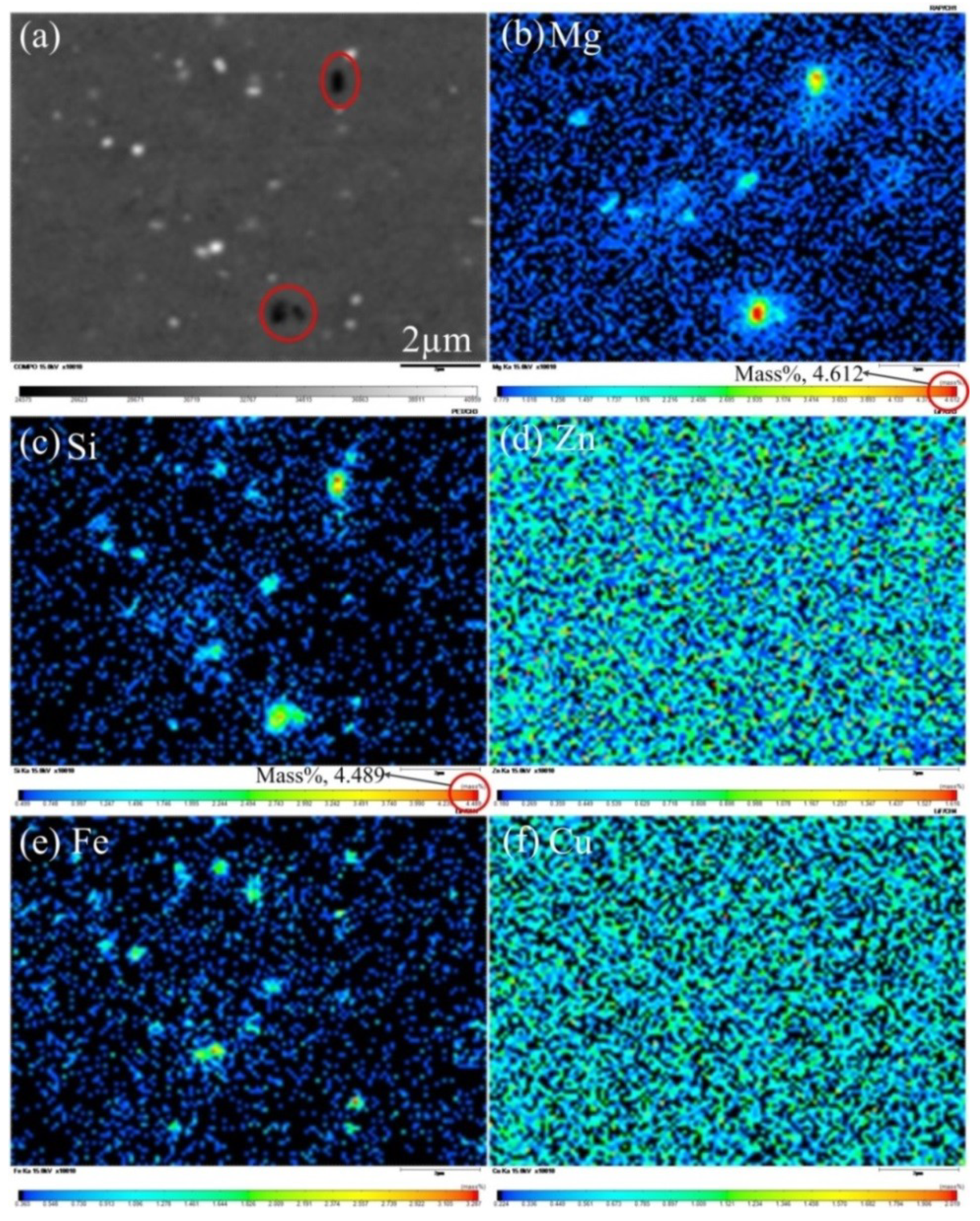
4.2. Verification Experimental Results

Considering that the solution of Mg and Si elements can strengthen the alloy matrix, the hardness measurement is a good way to characterize their solid solution strengthening effects [11]. Figure 9 shows the effects of SHT time on the hardness of 6061 aluminum alloy samples heated by conduction heating. After quenching, the hardness of the central zone was low because the Mg–Si precipitates dissolved or partially dissolved and the alloy was in a supersaturated solid solution containing oversaturated vacancies and supersaturated solutes [5]. After aging, the hardness of the central zone increased because Mg–Si precipitates formed. In addition, when the holding time was from 3 to 10 s, the hardness of the samples increased with the holding time, and then the hardness of the samples remained stable when the holding time increased from 10 to 15 s. In addition, the hardness of the samples before aging also remained stable when the holding time was more than 10 s. This means that the precipitates dissolved [11]. The results of the experiments indicate that it takes about 10 s for the precipitates in 6061-T6 aluminum alloy to dissolve at 560 °C under conduction heating during SHT. In the study by Maeno et al. [29], the SHT time of a 6061 aluminum alloy sheet under conduction heating was about 3 s, which was close to the experimental result in this work. In the work of Zhang et al. [11], experiments showed that it takes 15 s at 555 °C for the precipitated phase to dissolve in an Al–Mg–Si–Cu alloy, which is closer to our results.

According to the simulation results, the dissolution time of the precipitates was 11.6856 s, which was close to the experimental results. The error was about 16.7%. There are many factors that cause errors, some of the main factors being the initial size of the precipitation phase, the radius of the spherical space, the concentration in the matrix, and the diffusion coefficients of the atoms. There are also some assumptions, as mentioned in Section 2.1. Therefore, there must be some errors in the simulation results and the model should be improved.

At the same time, given the fact that it took about 10 s for the precipitates in 6061-T6 aluminum alloy to dissolve at 560 °C under conduction heating, the determination of the initial radius of the precipitates was not based on the size of the precipitates at 560 °C, which is why the precipitates may have dissolved or the size of the precipitates became smaller. That is why the size of the precipitates at 530 °C was used in the simulation. To sum up, the simulation results are reasonable and are expected to provide a guide for SHT of the 6000 series aluminum alloys in the industry.

5. Conclusions

(1) A precipitate dissolution model based on the mobile nodes method was established, and the solution process of the model was optimized as well. A flowchart of the modeling was also designed.

(2) The simulation of the isothermal dissolution of precipitates in a 6061 aluminum alloy sheet during the solution heat treatment process was conducted with the explicit finite-difference method based on the established model and flowchart.

(3) Conduction heating experiments were carried out to validate the numerical model. They indicated that the dissolution time of the precipitates in 6061-T6 aluminum alloy at 560 °C is about 10 s at a heating rate of 5 °C/s.

(4) The simulation results showed that the isothermal dissolution time of precipitates in 6061-T6 aluminum alloy at 560 °C is 11.6856 s. The dissolution time of the precipitate in the simulation was close to the experimental results, with an error of 16.7%, indicating that the modeling based on the mobile nodes method and the finite-difference method in this study is fairly reasonable and accurate. The error was caused by many factors, and the model should be improved.

References

1. Chandla, N.K.; Kant, S.; Goud, M.M. Mechanical, tribological and microstructural characterization of stir cast Al-6061 metal/matrix composites—A comprehensive review. Sādhanā 2021, 46, 47. [Google Scholar] [CrossRef]
2. Ghiotti, A.; Simonetto, E.; Bruschi, S. Influence of process parameters on friction behaviour of AA7075 in hot stamping. Wear 2019, 426–427, 348–356. [Google Scholar] [CrossRef]
3. Raugei, M.; El Fakir, O.; Wang, L.L.; Lin, J.G.; Morrey, D. Life cycle assessment of the potential environmental benefits of a novel hot forming process in automotive manufacturing. J. Clean. Prod. 2014, 83, 80–86. [Google Scholar] [CrossRef]
4. Geng, H.; Wang, Y.; Wang, Z.; Zhang, Y. Investigation on Contact Heating of Aluminum Alloy Sheets in Hot Stamping Process. Metals 2019, 9, 1341. [Google Scholar] [CrossRef] [Green Version]
5. Liu, Y.; Zhu, Z.J.; Wang, Z.J.; Zhu, B.; Wang, Y.L.; Zhang, Y.S. Flow and friction behaviors of 6061 aluminum alloy at elevated temperatures and hot stamping of a B-pillar. Int. J. Adv. Manuf. Technol. 2018, 96, 4063–4083. [Google Scholar] [CrossRef]
6. Chen, G.L.; Chen, M.H.; Wang, N.; Sun, J.W. Hot forming process with synchronous cooling for AA2024 aluminum alloy and its application. Int. J. Adv. Manuf. Technol. 2016, 86, 133–139. [Google Scholar] [CrossRef]
7. Sarafoglou, P.I.; Serafeim, A.; Fanikos, I.A.; Aristeidakis, J.S.; Haidemenopoulos, G.N. Modeling of Microsegregation and Homogenization of 6xxx Al-Alloys Including Precipitation and Strengthening During Homogenization Cooling. Materials 2019, 12, 1421. [Google Scholar] [CrossRef] [Green Version]
8. Yu, J.C.; Chen, Y.P.; Xu, G.L.; Wang, J. Dynamic mechanical properties and failure behavior on 6061 aluminum alloy annular forgings. Forg. Stamp. Technol. 2021, 46, 179–185. (In Chinese) [Google Scholar] [CrossRef]
9. Gussev, M.N.; Sridharan, N.; Babu, S.S.; Terrani, K.A. Influence of neutron irradiation on Al-6061 alloy produced via ultrasonic additive manufacturing. J. Nucl. Mater. 2021, 550, 152939. [Google Scholar] [CrossRef]
10. Liu, Y.; Zhu, B.; Wang, Y.L.; Li, S.Q.; Zhang, Y.S. Fast solution heat treatment of high strength aluminum alloy sheets in radiant heating furnace during hot stamping. Int. J. Lightweight Mater. Manuf. 2020, 3, 20–25. [Google Scholar] [CrossRef]
11. Zhang, X.K.; Guo, M.X.; Zhang, J.S.; Zhuang, L.Z. Dissolution of Precipitates During Solution Treatment of Al-Mg-Si-Cu Alloys. Metall. Mater. Trans. B. 2016, 47, 608–620. [Google Scholar] [CrossRef]
12. Whelan, M.J. On the kinetics of precipitate dissolution. Metal Sci. J. 1969, 3, 95–97. [Google Scholar] [CrossRef]
13. Brown, L.C. Diffusion-controlled dissolution of planar, cylindrical, and spherical precipitates. J. Appl. Phys. 1976, 47, 449–458. [Google Scholar] [CrossRef]
14. Cheng, L.M.; Hawbolt, E.B.; Meadowcroft, T.R. Modeling of dissolution, growth, and coarsening of aluminum nitride in low-carbon steels. Metall. Mater. Trans. A 2000, 31, 1907–1916. [Google Scholar] [CrossRef]
15. Zuo, Q.; Liu, F.; Wang, L.; Chen, C.F.; Zhang, Z.H. An analytical model for secondary phase dissolution kinetics. J. Mater. Sci. 2014, 49, 3066–3079. [Google Scholar] [CrossRef]
16. Vermolen, F.J.; van der Zwaag, S. A numerical model for the dissolution of spherical particles in binary alloys under mixed mode control. Mat. Sci. Eng. A-Struct. 1996, 220, 140–146. [Google Scholar] [CrossRef] [Green Version]
17. Vermolen, F.J.; Javierre, E.; Vuik, C.; Zhao, L.; van der Zwaag, S. A three-dimensional model for particle dissolution in binary alloys. Comp. Mater. Sci. 2007, 39, 767–774. [Google Scholar] [CrossRef]
18. Vermolen, F.J.; Vuik, K.; van der Zwaag, S. A mathematical model for the dissolution kinetics of Mg2Si-phases in Al-Mg-Si alloys during homogenisation under industrial conditions. Mat. Sci. Eng. A-Struct. 1998, 254, 13–32. [Google Scholar] [CrossRef]
19. Vermolen, F.J.; Vuik, K.; van der Zwaag, S. The dissolution of a stoichiometric second phase in ternary alloys: A numerical analysis. Mat. Sci. Eng. A-Struct. 1998, 246, 93–103. [Google Scholar] [CrossRef]
20. Chen, S.P.; Vossenberg, M.S.; Vermolen, F.J.; van de Langkruis, J.; van der Zwaag, S. Dissolution of β particles in an Al-Mg-Si alloy during DSC runs. Mat. Sci. Eng. A-Struct. 1999, 272, 250–256. [Google Scholar] [CrossRef]
21. Tang, Y.; Zhang, L.; Du, Y. Diffusivities in liquid and fcc Al-Mg-Si alloys and their application to the simulation of solidification and dissolution processes. Calphad 2015, 49, 58–66. [Google Scholar] [CrossRef]
22. Mohamed, M.; Foster, A.; Lin, J.G. Solution heat treatment in HFQ process. In Proceedings of the 12th International Conference on Metal Forming, METAL FORMING 2008, Krakow, Poland, 21–24 September 2008. [Google Scholar]
23. Van de Langkruis, J.; Kuijpers, N.C.W.; Kool, W.H.; Vermolen, F.J.; van der Zwaag, S. Modelling Mg2Si Dissolution in an AA6063 Alloy During Pre-heating to the Extrusion Temperature. In Proceedings of the 7th International Aluminum ExtrusionTechnology Seminar, Aluminum Extruders Council, Chicago, IL, USA, 16–19 May 2000; Volume 1, pp. 119–124. [Google Scholar]
24. Gui, Z.X.; Liang, W.K.; Liu, Y.; Zhang, Y.S. Thermo-mechanical behavior of the Al–Si alloy coated hot stamping boron steel. Mater. Design 2014, 60, 26–33. [Google Scholar] [CrossRef]
25. Österreicher, J.A.; Kumar, M.; Schiffl, A.; Schwarz, S.; Hillebrand, D.; Bourret, G.R. Sample preparation methods for scanning electron microscopy of homogenized Al-Mg-Si billets: A comparative study. Mater. Charact. 2016, 122, 63–69. [Google Scholar] [CrossRef]
26. Vissers, R.; Van Huis, M.A.; Jansen, J.; Zandbergen, H.W.; Marioara, C.D.; Andersen, S.J. The crystal structure of the β′ phase in Al-Mg-Si alloys. Acta Mater. 2007, 55, 3815–3823. [Google Scholar] [CrossRef]
27. Rometsch, P.A.; Arnberg, L.; Zhang, D.L. Modelling dissolution of Mg2Si and homogenisation in Al-Si-Mg casting alloys. Int. J. Cast Metal. Res. 1999, 12, 1–8. [Google Scholar] [CrossRef]
28. Sadeghi, I.; Wells, M.A.; Esmaeili, S. Modeling homogenization behavior of Al-Si-Cu-Mg aluminum alloy. Mater. Design 2017, 128, 241–249. [Google Scholar] [CrossRef]
29. Maeno, T.; Mori, K.; Yachi, R. Hot stamping of high-strength aluminium alloy aircraft parts using quick heating. CIRP Ann.-Manuf. Technol. 2017, 66, 269–272. [Google Scholar] [CrossRef]
Figure 1. Dissolution model of a spherical precipitate in an aluminum alloy during SHT and the interfacial movement under the control of diffusion: (a) the dissolution model of a spherical precipitate; (b) the interfacial movement model.
Metals 11 01234 g001
Figure 2. Re-meshing of the nodes after interfacial movement and the calculation of concentration.
Metals 11 01234 g002
Figure 3. Flowchart of the simulation for the precipitate’s dissolution.
Metals 11 01234 g003
Figure 4. Dimensions of the samples for conduction heating.
Metals 11 01234 g004
Figure 5. Micrograph of the 6061-T6 aluminum alloy sample heated by conduction heating (1, 2, 3, 4 and 5 indicate the precipitate’s serial number).
Metals 11 01234 g005
Figure 6. Element map of local area in Figure 5: (a) the local area; the element content of (b) Mg, (c) Si, (d) Zn, (e) Fe and (f) Cu.
Metals 11 01234 g006
Figure 7. Radius of the precipitate and dissolution velocity vs. time during dissolution.
Metals 11 01234 g007
Figure 8. (a) Mass concentrations of Mg and Si on the boundary changed with time. (b) Mass concentrations of nodes at the end of the calculation.
Metals 11 01234 g008
Figure 9. Effects of SHT time on the hardness of 6061 aluminum alloy samples heated by conduction heating.
Metals 11 01234 g009