Abstract
X-ray microcomputed tomography has been gaining relevance in the field of cellular materials to characterize materials and analyse their microstructure. So, here, it was used together with finite element modelling to develop numerical models to estimate the effective properties (Young’s modulus) of aluminium alloy foams and evaluate the effects of processing on the results. A manual global thresholding technique using the mass as a quality indicator was used. The models were reconstructed (Marching Cubes 33), then simplified and analysed in terms of mass and shape maintenance (Hausdorff distance algorithm) and face quality. Two simplification procedures were evaluated, with and without small structural imperfections, to evaluate the impact of the procedures on the results. Results demonstrate that the developed procedures are good at minimizing changes in mass and shape of the geometries while providing good face quality, i.e., face aspect ratio. The models are also shown to be able to predict the effective properties of metallic foams in accordance with the findings of other researchers. In addition, the process of obtaining the models and the presence of small structural imperfections were shown to have a great impact on the results.
1. Introduction
There have been some attempts to include aluminium alloy foams in mechanical design, such as crash-absorbing elements in vehicles (e.g., foam sandwich panels, foam filled thin wall tubes [1,2,3,4]), parts for milling machines and train prototypes, all taking advantage of the strength-to-weight ratio of the foams and their ability to absorb energy. Nevertheless, these are just the initial steps in the introduction of this type of material in the industry, seeing that their production is usually inconsistent, to an extent. The final properties depend on the internal cellular structure, which in turn depends greatly on (aspects of) the manufacturing process. The conventional methods (direct and indirect foaming methods) are usually used to prepare stochastic foams, i.e., foams with a random cell distribution, but new technologies (e.g., 3D printing) can already produce periodic cellular structures.
The mechanical characterization of metallic foams is an expensive process and each specimen is destroyed and can no longer be used. It is usually performed using experimental compression analyses, in which a specimen of a foam is compressed and its properties are extrapolated [5,6,7]. As a result, several analytical models and models based on Representative Volume Elements (RVE) have been developed to predict the mechanical behaviour of cellular solids [8]. However, they are just approximations, are usually periodic and don’t take micro-defects and small structural imperfections into consideration. For that reason, here, X-ray micro computed Tomography (CT) scans are used to construct 3D models to evaluate the mechanical properties of aluminium alloy foams, with special emphasis on the Young’s modulus, which bring much more detail and result, in theory, in a more exact analysis when compared to analytical models or models that use artificial/approximated geometries [9]. These sorts of methods are commonly used in the medical field, material science, engineering and are being introduced in the field of cellular materials, despite the research on the topic still being limited and there being little standardization [10,11,12,13,14,15,16,17,18].
2. X-ray Microcomputed Tomography and 2D Slice Analysis
X-ray microcomputed tomography (CT) allows the observation and study of the microstructure of foams and their virtual 3D representation, which has been the focus of most of the available research up until now [19]. However, its application combined with Finite Element Analyses (FEA) brings great potential and has been documented by some authors in varying degrees [11,12,13,14,15,16,17,20,21]. Through CT scans, 2D projection images are obtained, in which each pixel represents the level of attenuation of X-rays during scanning on an 8-bit grey scale, i.e., from 0–255 or 256 different values of grey ( = 256) [22]. Afterwards, they are used to mathematically reconstruct a 3D volume that represents the real foam specimen. This 3D representation could also be interpreted as a stack of 2D slices, or 2D reconstructed images, which facilitates the analysis and observation of details in the interior of the specimen.
There are many variables involved in such a technique and each could significantly change the end result. Therefore, it is difficult to obtain consistent results even for the same specimen when considering different users or different commercial CT scanners. For that reason, all necessary details are provided. Here, a SkyScan 1275 (Bruker, Belgium) scanner was used to acquire the geometries of three foam specimens: one cubic open-cell (Cubic OC, ≈ 22.8 × 22.4 × 19.5 mm); one cylindrical open-cell (Cylindrical OC, diameter: ≈19.0 mm, height: ≈20.0 mm); and one closed-cell (CC, ≈ 14.0 × 14.5 × 15.6 mm) (Figure 1a–c). The scan parameters, the properties of the base material and the final properties of each specimen are given in Table 1. The closed-cell foam specimen had been cut previously and the mass had to be approximated. The approximation was performed with the original volume and the final after-cutting volume (proportion of 39.5%). Assuming the material is homogeneous, the same proportion is applied to the mass. Additionally, a large crack along the foam was identified which seemed artificial (Figure 1d). Its origin is unknown but is suspected to be the process of cutting. The presence of such a defect could influence the results, however, it is not clear and the unavailability of another specimen restricts the options.
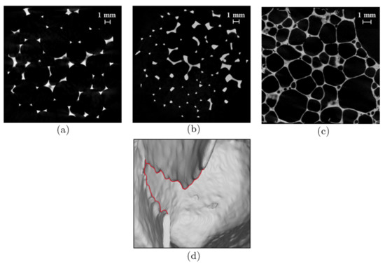
Figure 1.
2D slices of the (a) cubic open-cell foam, (b) cylindrical open-cell foam and (c) closed-cell foam specimens. (d) Section of crack identified in the closed-cell foam specimen.

Table 1.
Scan parameters, properties of the base material and final properties for the closed-cell (CC), cubic open-cell (Cubic OC) and cylindrical open-cell (Cylindrical OC) foam specimens.
2.1. Thresholding Techniques
An image, or 2D slice, I, can be defined in the form of a 2D ordered matrix of integers, i.e., it is a 2D function that maps from the domain of integer coordinates that form a bitmap image to a range of possible pixel values such that [22]
In this case, the value of each pixel is indicated on an 8-bit grey scale, i.e., from 0–255 or 256 different intensities of grey (). Thresholding or image binarization/segmentation is then an essential step, in which the different phases/constituents are distinguished using thresholding algorithms which measure the grey scale values in the 2D CT reconstructed images [23]. In other terms, these techniques transform images from levels of grey to binary (black and white) by finding an appropriate threshold, k. Essentially, the key question is how to find a suitable or optimal threshold k that best separates the background from the foreground, foam, while preserving the shape and minimizing the appearance of speckles. All operations were perfomed in CTAn (Bruker, Kontich, Belgium, v1.17.7.2) and an appropriate region/volume of interest (ROI/VOI) was defined which contains the whole specimen so that the whole specimens are included for further analysis of the mass.
The Otsu thresholding is the first technique tested. It is a global technique, has shown great reliability, simplicity and adaptability along the years and it is still the most used in image processing [23]. It determines an optimal threshold of an image by minimizing the within class variance, i.e., the background and foreground/object classes, using only the grey scale histogram of the image, therefore, it is a statistical approach [24]. In addition, it is used, in its primary form, to separate images with bimodal characteristics, i.e., images with two main peaks in the histogram and it works unsupervised, since no human interaction is needed to define any parameter [25]. Other similar thresholding techniques also exist, for example, multi-level thresholding, but aren’t considered here [26].
The Otsu thresholding technique was applied to the foam specimens considering the information of all slices, in 3D. This way, the calculations are done with the histogram of the sum of all the pixels of the series of reconstructed images (2D slices). Results show that for reconstructed images with clear borders there is good separation between the background and foreground which provides a clear visualization and understanding of the regions of interest of the specimen (Figure 2a). However, for regions with more noise or less differentiation between classes, there are many slight imperfections and a many small defects, creating a demand for more intense post-processing. Another disadvantage of this process is that it simply relies on information regarding the 2D slices. No external information is introduced. For these reasons, this technique might not be ideal.
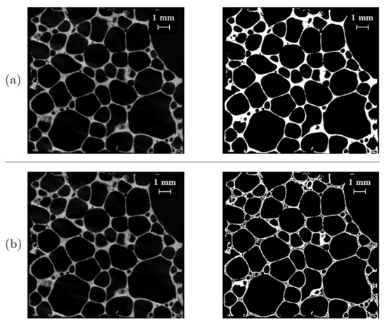
Figure 2.
(a)Application of the Otsu thresholding technique in 3D, which yields a threshold k of 70, and (b) application of the Mean-C technique (Radius of 2 and constant of 5) to the closed-cell foam specimen.
Contrasting to the global thresholding, for local or adaptive thresholding (AT) techniques, the threshold, k, is derived for each individual pixel by taking the values of the surrounding pixels in a specified region, i.e., the original image is divided into smaller areas. This definition could at first sight seem better for the final result since it takes local differences in the reconstructed images into consideration. However, it usually requires human intervention to define certain parameters and takes longer to calculate the results. AT techniques are commonly used to investigate a wide range of aspects related to the biology of bones and other calcified tissues and for scenarios with the presence of lightning gradients [23,25].
Mean-C, Median-C and Mean of Minimum and Maximum Values are some examples of AT techniques. All of them work with the same principle, despite presenting small differences. In essence, these techniques go through all pixels, and perform calculations with respect to the pixels inside a defined area, if considering a 2D image, or volume if considering a stack of images. This area/volume can be imagined as a matrix and can be selected to have a rather flexible shape, however, for more consistency, square/cuboid or circular/spherical/cylindrical shapes are usually used. In the case of the Mean-C, the mean of the values inside the defined area/volume around each pixel is calculated and a constant, C, a user specified value, is subtracted to it, obtaining the threshold. The Median-C and the mean of the min and max values techniques are similar to the one described, however, instead of calculating the mean of all values, they calculate the median and the mean of the minimum and maximum values within the defined area/volume, respectively. All the AT techniques require human intervention, unlike the Otsu thresholding technique, to select not only the size and shape of the selected area/volume, but also the value of the C constant. For these reasons, there are many fluctuations in the results.
The application of AT versus Otsu has been well documented for open-cell foams, where the foam morphology is analysed with respect to the applied technique [25]. The mean of the minimum and maximum values was mainly investigated and it was verified that some artificial pores appear in the struts of the foams and that the technique and its parameters impact the strut diameters greatly. The same outcome is verified here for the open-cell foams as well as for the closed-cell foam for all techniques and not just the minimum and maximum technique (Figure 2b). Results demonstrate that the presence of such voids in the walls and struts eliminates mass and changes the structure of the foam, which is detrimental, especially, for structural analysis. Moreover, defining the correct parameters is also very difficult because there are many possible combinations. Consequently, this type of technique is discarded as a viable option.
Another alternative is to apply a manually selected global threshold to the 2D slices. This technique, unlike the others, allows the user to consider and introduce external properties in the calculation process of the ideal threshold. Therefore, it isn’t solely limited by the properties of the 2D slices which are being analysed and provides a great opportunity to have more control over the process through the implementation of a quality indicator. However, it is difficult to gather and select information that could be used to verify the correctness of the results. In the case of foams, there is little information regarding the topology, or architecture of the real structure, and the shape, except the information that is gathered from the scans. However, the images obtained from the scans are also influenced by the scans themselves. Therefore, choosing a physical property of the real foams as a reference might be ideal. It can be contrasted with the outcome of the 2D slices and used to evaluate the results. In this scenario, it is a good choice to compare the real mass to the mass obtained after thresholding for each specific value of threshold. The threshold that yields the lowest difference between the real and virtual masses is, therefore, the ideal choice and the one that should minimize differences in the geometry. Consequently, there is at least some certainty that the virtual foam has the same amount of matter as the real one, therefore, having more chances of behaving like one during mechanical analysis. Thus, the mass of the foam is considered as the new quality indicator. For that purpose, sensitivity analyses were performed. The goal is to find if there is a relation between the two variables of interest, the threshold, k, and the mass measured in the software (CTAn, Bruker). The volume is interchangeably used with the mass since they represent the same thing, assuming a constant material density. Using the volume, , doesn’t require several conversions, therefore, it is preferred.
Thresholding Results
For the cubic open-cell foam, results show that for increasing threshold values both the foam volume and the foam surface area decrease. Figure 3a further clarifies this fact and shows an almost linear relationship between both parameters. However, for low levels of k, small noise/speckles are picked up, therefore, creating a slightly curved line which is easily fitted with a logarithmic tendency curve (in MS Excel version 16.0) (Figure 3). As seen in Table 1, the expected volume of the matrix material for this foam, , which weighs 1.100 g, is 411.991 mm. Solving the equation of the fitted tendency curve for k, a threshold of 90 was obtained which provides a volume of 413.202 mm. Given the obtained value is an approximation, the value above, , was tested, yielding a volume of 411.410 mm, which corresponds to a very small difference of 0.141% of the real volume. Therefore, results indicate that for this foam the process was very successful in maintaining at least the same amount of material as the real foam.
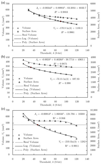
Figure 3.
Threshold sensitivity analysis for the (a) cubic open-cell, (b) cylindrical open-cell and (c) closed-cell foam specimens. Red point represents intersection of real volume with the volume curve.
The same procedure was repeated for the cylindrical open-cell foam specimen using the values in Table 1. The final value obtained for the threshold, k, was 32, consequently leading to a volume of 341.291 mm, which corresponds to a difference of 0.138% of the real foam volume (Figure 3b). Comparing both specimens, there is a clear distinction in the value of the thresholds even though their structure is similar. So, regardless of the number of specimens, it is safe to assume based on the results and visual breakdown of the slices of each foam that the value of the threshold depends greatly on the CT scan parameters.
The same analysis was performed for the closed-cell foam using the properties summarised in Table 1. An almost linear relation is again verified in the middle range of the scale, however, the effect of the speckles and noise is again present for lower levels (Figure 3c). The surface area shows a less predictable behaviour. An ideal threshold is found to be 47, which yields a volume of 474.056 mm, i.e., a variation of 0.108%. In contrast, the Otsu technique yields a variation in the final volume/mass of 15.048% (with a threshold of 70) and the Mean-C technique a variation of 32.877% (with a radius of 2 and a constant of 5, for example). Hence, the manual selection of the threshold based on the quality indicator is preferred.
2.2. Closing Morphological Operation
The presence of small defects and very small pores can sometimes be unwanted and problematic for the next stages of acquiring the geometry of a foam. Morphological operations, more specifically, the closing operation, are a very good tool to avoid these sorts of problems and make the surfaces more regular, maintaining, for the most part, the shape and architecture of the structures. It also brings some loss of information to the process and the values of threshold for the same volume can be different because of the closure of pores, which increases the amount of mass in play. The closing operation is a complex operation composed by a dilation followed by a erosion. For open-cell foams, the effects are not obvious, while for the closed-cell foams the impact is meaningful and the effects are (Figure 4): (i) Pores smaller than the structuring elements are closed; (ii) surfaces are smoothed; (iii) some holes in the walls of the pores are closed [22]. The effects are, for the most part, desirable, however, the changes in topology, addition of material and changes to its distribution can be significant and finally alter the behaviour of the geometry when placed under loads during a finite element analysis. Nevertheless, it makes it easier to process the geometry in subsequent steps and reduces the number of kinks and areas of stress concentrations.
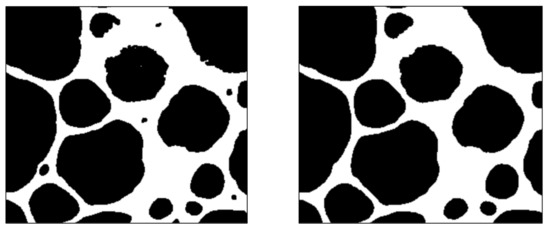
Figure 4.
Ideal threshold with no morphological operation (left) and ideal threshold for a morphological operation of radius 6 (0.09 mm) (right) for the closed-cell foam specimen.
For this reason, a sensitivity analysis was performed for approximately spherical structuring elements, chosen because of the shape of the pores. Caution is required when using such operations due to the fact that specimens with smaller image pixel sizes, i.e., with a higher number of pixels per a given area, yield different results when comparing with specimens with larger image pixel sizes. This issue originates from the definition of the structuring element which is, in simpler terms, a matrix/filter that runs through all the pixels of the image. As a consequence the real radius of the operation is also provided,
where R is the radius of the structuring element in the real world, r is the radius in terms of matrix sizes and is the image pixel size, which is 15.001 m for the closed-cell foam (Table 1).
Results indicate that as the radius of the morphological operation increases, the final volume also increases while providing the smoothing and closure of small pores as discussed before. This effect can be easily verified by the stacking of curves starting from the smaller radius, i.e., with no closing operation, to the higher radius in Figure 5.
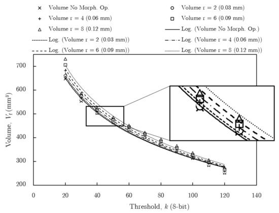
Figure 5.
Sensitivity Analysis for different radii of the structuring element.
For each different curve a new ideal threshold and its corresponding values were calculated (Table 2). Larger structuring elements could have been used, however, the computational time increases exponentially and the shape of the final foam would change even further.
Table 2.
Ideal thresholds for the closed-cell foam specimen with different morphological operations. The error (%) in volume with regard to the real foam is also given.
3. 3D Geometry Simplification and Analysis
The binarized 2D slices are usually used to reconstruct a 3D model in STL which accurately represents the real specimen (Figure 6). Nevertheless, the obtained 3D model, or surface mesh, or boundary mesh is flawed, i.e., it has too many nodes and several small errors, and must be corrected and simplified so that it can be utilised in Finite Element Method (FEM) analyses. However, some difficulties emerge, namely that the simplification procedure itself can have a major impact on the final results. For that reason, two different simplification procedures are discussed. The first seeks to maintain all the small details, defects and cracks that connect pores in an attempt to more accurately replicate the real foam specimens. The second aims to eliminate those features to make the model more stable and smooth by targeting and eliminating faces with high discrete curvature. In addition, the involved algorithms were selected for their ability to cause meaningful yet minimal change to the structure of the foams.
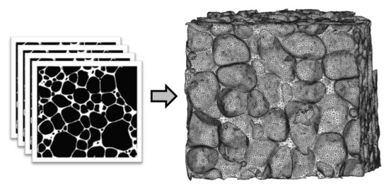
Figure 6.
Conversion of binary slices to fully processed 3D model.
The resulting 3D models are tested to ensure the simplification was done successfully and with minimal loss of information. They are tested in terms of mass/volume preservation and shape preservation with the Hausdorff distance and the distance between meshes algorithm. The tests provide reassurance that the final 3D models are, in fact, correct and that the procedure of reconstruction and simplification was well done (Figure 6). Similar research has been done in order to acquire the 3D models for FEM simulation, however, the effects of the process were not investigated and few control variables were presented, such as the evolution of the mass or changes in the shape [11,12,13,15,16,17,18]. Hence, these topics are given a greater focus.
3.1. Reconstruction Algorithms
In spite of there being many methods that can perform the reconstruction of the models using the 2D slices, here two of them are explored more thoroughly, using CTAn: Marching Cubes 33; and Double-Time Cubes.
The Marching Cubes 33 algorithm (MC33) is used for the reconstruction of isosurfaces from volumetric datasets, i.e., from 3D arrays of data [27,28]. It uses the images obtained with the CT to create a surface representation. Initially, these methods were applied for rendering in medical applications, however, they can be applied in many other areas, e.g., to obtain models to be used in structural analysis and 3D printing. This technique uses a divide-and-conquer approach to locate the surface in a logical cube from eight pixels, four from one 2D slice and four from another adjacent slice/image. The algorithm determines how the surface intersects this cube and then moves, marches, to the next cube. As the name implies, there are thirty three different intersection patterns that a surface could present.
The other alternative is the Double-Time Cubes algorithm (DTC) which, according to Bruker, produces very similar results to the MC33 [29]. However, results show that the final mesh shows a reduction of 50% in the number of faces and a smoother surface, or boundary mesh, which is better for visualization. Nevertheless, the smoothed surface is produced without human interaction which might lead to uncontrolled loss of information.
The primary goal is to minimize losses of information along the process, so the final volume, or mass, of both structures for both methods was compared to the real value of the real specimen. Taking the cubic open-cell foam as an example, the values of interest can be analysed in Table 3. An error of 8.029% of the volume for the DTC is verified which is easily defeated by the MC33 with an error of only . The MC33 maintains the volume/mass constant and preserves more information. This can also be observed by the variation of the surface area that shows a small change of 0.301% in contrast to 6.633% for the other method. Moreover, the number of faces is the double for the MC33 algorithm. On one hand, more faces mean more details. On the other hand, the file is bigger and its processing time is larger. Nevertheless, the high amount of details is preferred and the file can later be simplified on command and not just randomly by the surface reconstruction algorithm. Despite the given example being just for the open-cell foam specimen, the same results are observed for the closed-cell foam and cylindrical open-cell foam specimens. For that reason the MC33 is applied to all foam specimens (Table 3) with an error estimation considering the real foams’ volumes/masses. Given there is no information regarding the real surface areas, the variation included refers to the one obtained with the software. The values of that parameter for the cylindrical open-cell and closed-cell foam show a large, unjustified variation, however, when the geometries suffer a reduction in the amount of faces, the values become similar to what is expected. This is due to the large number of faces, 49 and 89 million for the cylindrical open-cell specimen and for the closed-cell specimen, respectively, in Meshlab (v2016.12, www.meshlab.net) [30]. This effect was neglected in both cases since the main focus is the volume/mass.
Table 3.
Comparison between the Double-time Cubes and the Marching Cubes 33 algorithms. The error in volume with respect to the real values is provided between brackets. The error in surface area is calculated with the values obtained with CTAn.
3.2. Main Simplification Algorithms
The reconstructed 3D models usually exhibit some errors which need to be corrected, for example: (i) gaps, i.e., missing faces or holes; (ii) degenerate faces, i.e., where all its edges are collinear; (iii) overlapping faces or self-intersecting faces; (iv) non-manifold topology conditions, i.e., non-manifold edge, point and face.
There are many different algorithms which could be applied to simplify and correct the obtained surface/boundary meshes, each yielding different results. Therefore, the employed algorithms were the ones that presented the most consistent results in Meshlab. The four main ones used were:
- (i)
- Quadric edge collapse decimation;
- (ii)
- Taubin smooth;
- (iii)
- Close holes;
- (iv)
- Discrete curvature calculation.
Each one was selected due to its ability to cause meaningful change to the mesh while preserving the shape and not causing significant shrinkage, i.e., volume reduction.
3.2.1. Quadric Edge Collapse Decimation
The quadric edge collapse decimation algorithm is the most important for the simplification of the mesh, i.e., reduction of the amount of faces. This technique is very important in the context of models built based on CT-imaging since they are usually oversampled and very taxing for computers. It is able to perform the desired simplification while maintaining the volume of the model and keeping sharper features, to a certain degree. Such characteristics make it an ideal solution for the problem at hand. This algorithm simplifies the mesh based on Quadric Error Metrics (QEM), as opposed to others that use the geometric distance, which allows for the preservation of features with high curvature [31]. To perform the simplification, a mechanism named edge collapse is applied [32]. There are also other methods for the simplification of a mesh, such as vertex clustering [33], vertex decimation [34], etc.
The algorithm has many options and parameters which could be used. Therefore, in Meshlab, the parameters were selected based on the recommendations of the software, with boundary preservation, topology preservation, planar simplification, optimal positioning of simplified vertices, a quality threshold of 0.4 (0–1, 0.5 penalizes good faces) and the intended final number/percentage of faces. An analysis of the effect of different values was not performed, however, it is important and should be the target of greater focus in the future. Results show that reducing the number of faces up to 98% of the initial number yields a minimal error in volume and surface area of around 2% and 10%, respectively, for the available specimens. The face quality, i.e., aspect ratio, was reduced due to the collapse of edges, which was handled with a smoothing operation described in the next section, where the analysis of the face quality is also performed.
To generalize the analysis of the foams in terms of the number of faces and to make it clearer for future work, the density of faces is used instead of the pure amount from this point onwards. For this purpose, the face density, , is defined as the number of faces, , divided by the volume of the bounding box, , of each foam as:
3.2.2. Taubin Smooth
The Taubin smoothing operation provides a method to regularise faceted geometries of arbitrary topology while keeping the changes in volume and in shape to a minimum, i.e., it doesn’t produce shrinkage. Additionally, the face quality is also improved, making each face more regular and closer to an equilateral triangle [35,36]. Here, it is given great importance due to the fact that it facilitates the application of other algorithms and prevents the genesis of subsequent errors, e.g., bad mesh simplification using the quadric edge collapse decimation and difficulty in FEM mesh generation.
The algorithm was applied in Meshlab using empirically selected parameters based on the recommendations of the software. They were selected so that no extreme changes to the model were verified. , the scale factor for the shrinking step, was selected to be 0.5, despite higher values, e.g., 0.6, yielding smoother surfaces. 0.55 for , the negative scale factor for the un-shrinking step, due to , and 10 smoothing steps/iterations.
The theory of this smoothing process translates very well into reality. It manages to produce very minimal shrinkage, the shape is preserved and the number of faces remains the same. For example, applying this algorithm to the cubic open-cell and closed-cell foam specimens produces a very small variation of volume of just 0.04% and 0.09%, respectively. Such range of values is negligible. Regarding the quality, the effects can be seen in Figure 7, a cut version of the closed-cell foam, where the application of the algorithm causes very visible changes to the quality of the surface making it more regular. Here, the quality is calculated as [37]
where inscribed radius is equal to the radius of the largest circumference that fits inside a triangle, circumscribed radius means the radius of the circumference that contains the triangle vertices and K has been chosen so that the equilateral triangle has . In the histograms of Figure 7, there is a clear shift of the values towards levels of higher quality, i.e., faces with quality equal to 1, (the size of the bars of the histogram are scaled to allow for better visualization). The mean value changes from 0.75 for the initial mesh to 0.84 for the post smooth surface.
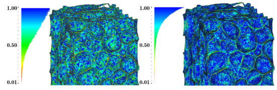
Figure 7.
Comparison of surface quality before (left) and after smoothing (right) for the closed-cell foam specimen. Histograms bars are adjusted to a max size.
3.2.3. Close Holes
One of the most essential steps of simplifying and repairing the 3D models is to close the holes, or gaps, which are a consequence of missing faces and one of the main problems, turning them into a closed manifold mesh. The elimination of such gaps follows the following strategy [38,39]: (i) Check for approved edges with adjacent faces; (ii) Detection of gaps in the tessellated model; (iii) Sorting bad edges into closed loop; (iv) Generation of faces for the repair of gaps. More complex gaps can be solved using Autodesk Meshmixer (San Rafael, CA, USA, v3.5.474).
3.2.4. Discrete Curvature
Because of the definition of the 3D models based on triangle surface meshes, there is no intrinsic curvature. They are inherently discrete and each face is planar. However, the discrete curvature calculation algorithm is able to extract an approximation [40]. The obtained curvatures by this calculation allow the detection of very small features, which could cause problems during meshing for FEA, and also find small defects and cracks in the cell walls, that could significantly change the strength of a foam.
This algorithm was applied in Meshlab in the RMS (Root Mean Square) variation. In this software, the curvature is calculated for each vertex and saved in the vertex quality field. From the stored values, vertices can be selected based on their curvature values. For example, in order to eliminate very small features, all vertices with quality equal or higher than 300 (empirical value) were selected and eliminated (working in millimetre). Another option is to select and eliminate all vertices with curvature higher than 30–40 (empirical values) in order to eliminate the areas of small cracks and defects on the cell walls for subsequent remeshing. Many other vertices could also be unintentionally included in the selection with the curvature, however, it can also be easily solved with the hole closing algorithm.
3.3. Simplification Procedure
The simplification procedure must be able to reduce the number of faces and eliminate all problems regarding STL meshes, for instance, gaps (cracks, holes), i.e., missing faces, degenerate faces, i.e., where all its edges are collinear, overlapping faces or self-intersecting faces and non-manifold topology conditions(non-manifold edge, point and face) [38,39,41]. In order to complete this task, several functions/algorithms are applied, some of which have already been described in previous sections, and the results are evaluated in terms of volume and surface area preservation and shape preservation. Then, the requirements for the final mesh are:
- (i)
- Closed manifold mesh, consequently, watertight;
- (ii)
- Free from self-intersecting faces;
- (iii)
- Reduced number of faces or reduced face density;
- (iv)
- Geometrically and topologically identical to the real foams;
- (v)
- Good quality, i.e., faces with a good aspect ratio and a low distortion/curvature.
Two different procedures were applied: (i) Procedure 1, or plain simplification; (ii) Procedure 2, or elimination of cell wall defects. These procedures are more focused on simplifying the closed-cell foam since it is more complex and nothing more than an extension of the preparation of the open-cell foam. Similar or better results could probably be obtained in another manner or in another order, however, the described procedures showed moderate implementation difficulty as well as consistent results.
Procedure 1 is designed to process and simplify the specimens, yielding a model that fulfils all of the requirements mentioned above. The main idea is to keep the shape and topology almost unchanged, including small structural imperfections and cracks, while applying the necessary simplifications. The process pipeline is shown in Figure 8. The Taubin smooth algorithm is applied in the beginning as well as the end since it facilitates the application of other algorithms. Vertices and faces with high discrete curvature (above, for example, 300, when working with millimetre) are deleted to remove very small features. The borders around the gaps in the models are eliminated several times since there are usually irregularities that make the gaps difficult to close. All other algorithms are applied as discussed in in previous sections. In the end, the boundary mesh should faithfully represent the original surface even including the very small defects and imperfections in the cell walls which connect different pores, in the case of closed-cell foams, since it is known that the physical properties of a foam are a direct consequence of their micro-/macro-structure [42]. So, their presence is normal, as verified in some articles, and desired in terms of fidelity to reality [43]. However, small defects are sure to originate kinks during FEA.
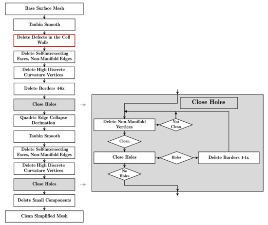
Figure 8.
Procedure pipeline. The step represented in red is only added for Procedure 2 (clean small defects and cracks).
It seems reasonable to extend the previous procedure to eliminate the aforementioned defects, or structural imperfections, in the cell walls and obtain an even smoother and cleaner surface which will be more stable during analysis. So, Procedure 2, i.e., elimination of cell wall defects, is introduced. Having both types of surface allows the observation of the magnitude of change caused by their elimination, how the results might be dependent on the process of obtaining and processing the surfaces and if there should be a stronger process standardization across this scientific field. Eliminating the small imperfections in Meshlab is a time-consuming process and depends on the experience of the user with the software. Nevertheless, the procedure is described for the closed-cell foams, given it is useless in the case of the open-cell foams because they show, in comparison, a low number of defects. To accomplish this objective, a method which detects their presence is required, given their position is completely arbitrary. Observing the defects and their shape, it can be verified that the areas involving them have high curvatures. Therefore, by taking advantage of this property, the faces can be deleted, leaving one gap on each side of the corresponding cell wall, which are later remeshed/fixed. For this purpose, the discrete curvature algorithm is applied again in the whole process as shown in Figure 8, maintaining the rest of the process pipeline unchanged. This time, all vertices with curvature values above a given threshold, usually around 30 to 40 (Empirical values, others could be used) when working with millimetre as the main unit, are selected in order to capture all the intended areas. For this reason, the user might be required to test different threshold values and check which works the best. The final result should be satisfactory and similar to Procedure 1, except for the presence of small defects (Figure 9).
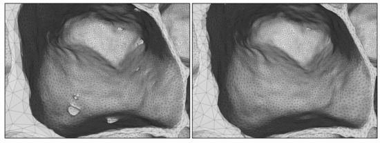
Figure 9.
Procedure 1 with defects (left) and Procedure 2 without defects (right).
3.4. Simplification Results
The analysis is performed in terms of mass/volume preservation and shape preservation with the Hausdorff distance algorithm and the distance from a reference mesh algorithm. The analyses were performed for the cubic open-cell foam and closed-cell foam specimens. The cylindrical open-cell foam is not included in the following analysis since it shows similar results to the cubic one and was mainly used to verify the effect of the different scanning parameters in the threshold. The cubic open-cell foam specimen was used in its entirety and was processed using a threshold of 91 and no closing operation. In contrast, due to the large number of faces of the closed-cell foam, i.e., 89 million, and, consequently, the high computational effort associated with them, only a section of the closed-cell foam specimen of 8 by 14 mm which extends in the z direction by the original amount of 15.571 mm was used. Reducing the size of the specimen should not be problematic since it is just used as a mean to evaluate the variation caused by the process of obtaining the simplified 3D model in the values and not because of the absolute values themselves. A threshold value of 47 and no closing operation were the defined parameters. In addition, the focus of this section is a foam which has been minimally processed, i.e., Procedure 1, where the smaller defects weren’t removed. This decision is mainly due to the fact that the results are similar and that the variation in volume/mass for Procedure 2 in comparison to Procedure 1 is minimal, ≈0.1%.
3.4.1. Mass/Volume and Surface Area
In the case of the closed-cell foam specimen, the error in volume increases almost exponentially for decreasing face densities hitting a maximum of around 2% for 286 faces per mm or 500 thousand faces, which corresponds to a reduction of about 99% of the initial amount, 26,136 faces per mm or 45.7 million faces (Figure 10). Regarding the surface area, a peak error of 43% is verified for the initial density of faces, however, the value converges to the value calculated by CTAn for smaller densities. A reason for this outcome was not found.
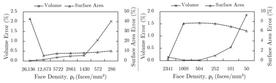
Figure 10.
Error of the volume and surface area with respect to the density of faces for the closed-cell foam (left) and the cubic open-cell foam (right).
For the cubic open-cell foam specimen, results show a similar behaviour to the closed-cell foam for the volume error with a maximum value of around 1.8% for a density of 50 faces per mm or 500 thousand faces, which corresponds to a reduction of about 98% of the initial amount, 2341 faces per mm or 23.2 million faces (Figure 10). The error of the surface area shows a more unstable development, where it initially increases to a maximum of around 8% and, subsequently, slightly decreases.
It can be concluded that the volume and, therefore, the mass evolves in a predictable way, showing low errors even for very high reductions of the number of faces for both open and closed-cell foams. The effect of the procedure on this parameter was minimal, so, it can be considered successful. On the contrary, the surface area is more unstable and there are some problems when calculating it. Even though it is not an essential parameter, more time should be dedicated to its analysis in the future. Regardless, the simplification of the meshes to very low levels still only exhibits a maximum error of 10%, which is acceptable.
3.4.2. Distance between Meshes
The analysis of the volume and the surface area is useful, however, it is not enough to confirm that the 3D models maintained their shape. For this reason, the Hausdorff distance algorithm and the distance from a reference mesh algorithm are applied, which provide statistics about the error distribution regarding the distance between a mesh to be measured and a reference mesh [30,44].
The Hausdorff distance was calculated using Meshlab for the closed-cell foam for several levels of face densities. The number of samples along the surface was selected to be equal to the number of vertices, ≈23 million, of the reference mesh, i.e., the initial mesh without any filter or smoothing operation. Given this method provides the one-sided average distance, the distance calculations were done for both sides and averaged, in order to facilitate the evaluation. Results demonstrate that for higher levels, the average shows an almost linear behaviour, however, it drastically increases for lower levels (Figure 11a). Even for a simplification of 286 faces per mm or 500 thousand faces, i.e., a reduction of 99%, the error is only around 0.032% of the diagonal of the bounding box, which corresponds to a maximum average distance of 0.07 mm. Additionally, the histogram with the colour map and the coloured mesh provide a very useful tool to analyse where the biggest differences appear. Here, the areas where the foam was cut show the largest variations in shape, while the rest maintain the initial format well.
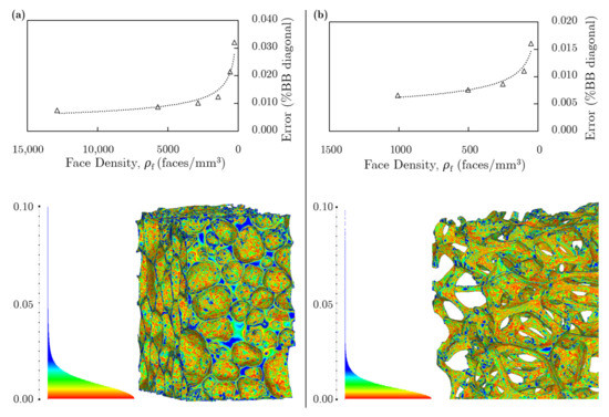
Figure 11.
Average of the two-sided Hausdorff distance and visual representation of the Hausdorff distance (a) of the cut closed-cell foam specimen and model with 500 thousand faces, i.e., 286 faces per mm and a 99% reduction, (b) and of the cubic open-cell foam specimen and model with 500 thousand faces, i.e., 50 faces per mm and a 98% reduction.
The same procedure was applied to the cubic open-cell foam specimen. The reference mesh was again the initial surface without any sort of processing. Figure 11b shows that the error, i.e., the average distance between the meshes as a percentage of the bounding box’s diagonal, has a similar behaviour to that of the closed-cell foam. It is close to linear for higher levels of density, however, in the case of lower levels, the error appears exponential. Still, even for a density of 50 faces per mm or 500 thousand faces, the error is only 0.016%, which corresponds to 0.006 mm.
The second applied algorithm, Distance from Reference Mesh, to test the similarity of the processed meshes to the initial one is very similar to the Hausdorff distance. The main difference is that it calculates the signed distance, i.e., positive or negative, instead of the absolute value. This technique works with the same principles as the previous one, however, the sampling is done vertex to vertex instead of uniformly distributed sampling points and the distance is signed.
For the closed-cell specimen, the results for every calculation show a normal distribution and the average is always very close to zero, therefore, it is complemented with the standard deviation. As it can be seen in Figure 12a, the mean and the standard deviation shift lightly for high face densities, however, for very low densities the mean starts to move away from zero and the deviation increases much quicker. For example for a density of 286 faces per mm or 500 thousand faces (99% reduction), the mean error has a value of −0.002% with a standard deviation of 0.045%. The obtained values are, therefore, low even for a very simplified structure. From the visual representation of the distance, also Figure 12a, since the distance is signed, there is a greater awareness about where the shape is changed and in what direction. In this case, the representation is of the distance calculated with the final mesh as the reference and the initial as the one to be measured. The only foreseeable consequence is that distances are inverted to what is expected, therefore, areas in the red spectrum represent points where the final mesh stays above the initial and in the blue spectrum the inverse. The red areas are mostly seen in planar surfaces, which are artificial and a consequence of cutting the foam, where the smoothing of the edges of the pores appears to cause these surfaces to lift. Blue areas are especially seen in thin walls and edges where their smoothing causes some contraction and rounding.
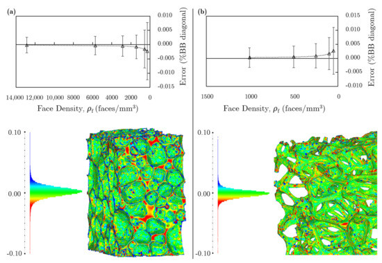
Figure 12.
Average distance from a reference mesh and visual representation of the distance from a reference mesh (a) of the cut closed-cell foam specimen and model with 500 thousand faces, i.e., 286 faces per mm and a 99% reduction, (b) and of the cubic open-cell foam specimen and model with 500 thousand faces, i.e., 50 faces per mm and a 98% reduction.
The calculations were repeated for the cubic open-cell foam, which shows very similar results to the closed-cell. The evolution of the error is close to linear for high face densities, however, it starts to move away from zero towards positive numbers for low densities, along with a great increase of the standard deviation (Figure 12b). Ultimately, the error is quite low, representing just around 0.003% with a standard deviation of 0.02% for a foam with 50 faces per mm or 500 thousand faces (98% reduction).
4. Numerical Modelling and Analysis
The obtained 3D models (boundary meshes) derived from the CT scans are submitted to Finite Element Analyses (FEA). The main purpose is to evaluate the effective relative Young’s modulus with respect to the relative density of the different types of foams when submitted to a compression loading scenario and, for the closed-cell foam, the influence of the procedure from the 2D slices to the simplified 3D model in the results. To evaluate the results, several theoretical and numerical models are used as a mean of comparison for the cubic open-cell foam [45,46,47,48,49,50,51,52,53] and closed-cell foam [8,51,52,53,54,55,56,57].
4.1. FEA Meshing and Boundary Conditions
Usually, in finite element analyses the parts are modelled parametrically, i.e., in a NURBS based format [58], and can be directly inserted into most simulation software. However, the foam parts in this work are saved in a different format, STL, which lacks some information, in comparison to the above mentioned, and is not recurrently accepted as an input format. Since converting the STL models into parametric models is usually limited by the number of faces and the size of the files, the direct application of STL model to obtain a FEA mesh is preferred. Using the mesh generator Gmsh (v4.5.2, www.gmsh.info) [59], a surface mesh, or boundary mesh, in STL format is introduced to create a volumetric finite element mesh which uses the faces of the initial boundary mesh as the external faces of the created tetrahedrons (3D elements), i.e., the creation of the 3D elements is tied to the boundary mesh, which could be considered a limitation [37,60]. Therefore, optimizing and creating a high quality STL takes on greater importance.
Regarding the boundary conditions, a loading scenario with Symmetry boundary conditions with an Imposed Displacement (SID) was chosen. Such a configuration enforces a displacement on one of the sides of the sample, places symmetry conditions on three other sides and leaves two perpendicular sides to the load direction free, which allows the calculation of the Poisson’s ratios and reaction forces (Figure 13). It is considered an homogenization approach, such as asymptotic expansion homogenization, among others [61,62]. Contrary to Symmetry boundary conditions with a Prescribed Force (SPF), where a force is imposed on one of the sides, SID provides better load homogeneity, especially since the geometries based on CT scans are irregular [53,61].
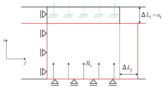
Figure 13.
2D representation of the SID boundary conditions.
The effective properties of the foam specimens can then be determined by applying Hooke’s Law [63]. The effective Young’s Modulus, E, is given by
where is the stress, is the strain, is the force, A is the area of the section of the specimen, is the displacement and the length of the specimen in the load direction. Considering the imposition of a displacement , as the displacement in a generic perpendicular direction to the loading direction and as the reaction force, the effective Young’s modulus and Poisson’s ratio take on the following forms:
The intention is to analyse each specimen in all three dimensions, but with the considered boundary conditions the cylindrical open-cell foam specimen is unusable. Adjustments would be necessary in order to extract the necessary values, therefore, it is left out.
4.2. Mesh Refinement
To study the mesh density is an essential step in the process of analysing the available foam specimens, in order to find a refinement level in which there is a good equilibrium between computational requirements and stability of the results. The conditions were defined as described above with an arbitrary imposed displacement of 1 mm and the error of convergence is calculated with respect to the value of the previous refinement level for all specimens [64].
Figure 14a shows the evolution of the error of the Young’s modulus with respect to the increase in the number of nodes for the cubic open-cell foam (Table 1). Initially with a size of ≈22.8 × 22.4 × 19.5 mm, the specimen was slightly reduced to ≈19.5 × 19.5 × 19.5 mm for all the following steps, in order to eliminate some irregularities in the extremities and to facilitate further calculations ( mm, ). It is possible to verify that for 750,000 nodes, or 2,250,000 degrees of freedom, which corresponds to Pa, the development of the Young’s modulus is minor and that there isn’t much benefit in using higher refinement levels. The small fluctuations observed in Figure 14a can be a result of the process of meshing which, in this case, is completely connected to the STL file that was used, i.e., the process is manual and can induce small changes in the geometries. Consequently, a satisfactory level of refinement of around 750,000 nodes has been found and is further used to analyse the specimen in subsequent sections.
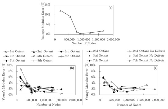
Figure 14.
Convergence analysis of the error of the Young’s modulus for the (a) open-cell specimen, (b) closed-cell foam specimen prepared with Procedure 1 and (c) closed-cell foam specimen Procedure 2 (no defects) compared with Procedure 1.
The closed-cell foam specimen (≈14.0 × 14.5 × 15.6 mm) is not ideal, i.e., it was cut before the CT scan, which caused some larger internal and artificial cracks, and its volume/mass was approximated (Table 1). For this reason and the large size of the foam file, the specimen was divided parallel to the three main plains, i.e., divided in octants, creating eight smaller parts of 8 × 8 × 8 mm with 3–6 pores in each main direction with small overlapping areas. Even though small amounts of pores can lead to unwanted effects or irregular behaviour and show different results when compared to larger amounts of pores, this separation allows for the observation of the consequences of the presence of the larger cracks [43]. In addition, the whole specimen was slightly reduced to ≈13.1 × 13.1 × 13.1 mm for all the following steps, in order to eliminate some irregularities in the extremities and to facilitate further calculations ( mm, ).
The octants were simplified with the two discussed simplification procedures: Procedure 1, i.e., plain simplification; and Procedure 2, i.e., elimination of cell wall defects and small structural imperfections. Each of them was reduced to 0.7%, 2%, 5%, 7%, 10% and 15% of its original number of surface faces, because the simplification is performed in Meshlab [30]. Results indicate that for Procedure 1 there are large discrepancies between the Young’s modulus errors of different octants (Figure 14b). Fluctuations are especially high, for example, for the fourth octant. Nevertheless, the error between each level decreases for increasing numbers of nodes, in spite of being irregular, and from the third level of refinement (from left to right), i.e., 5% of the original number of surface faces, there are no large changes. For that reason, that is the level of refinement which is used to study the close-cell foam specimen with Procedure 1.
For Procedure 2, only three octants were analysed due to the limited time frame and because they provide enough information (Figure 14c). The same irregular behaviour is observed for each part with no defects/kinks but with a clear decrease in error. Furthermore, from the third refinement level, 5%, there seems to be no great benefit in increasing the number of nodes. When comparing the analysis of the same octant with both procedures, the Young’s modulus shows a different convergence behaviour and, therefore, appears to be dependent on the process of simplification. However, the third octant did not show a different behaviour for the two methods, as their points in the graph are coincident, and their Young’s moduli are roughly the same. This phenomenon is unpredictable and can only be explained by the process of elimination of the defects in the cell walls not being successful or this section not having many or not so relevant structural imperfections. In conclusion, the 5% refinement level seems to be, again, a good trade-off between time/computational resources and quality of the analysis.
4.3. Results Cubic Open-Cell Foam
Figure 15a shows the effective relative Young’s Modulus of the cubic open-cell foam, obtained with the Procedure 1, plain simplification with respect to the relative density and compared to the analytical models [45,46,47,48,49,50,51,52]. It is possible to observe that the developed CT based model lands very closely to the expected values determined by the analytical models but slightly above them. This could be possibly explained by the lack of small cracks and structural imperfections, which are eliminated by the process of simplification, and are known to reduce the strength of the material [43]. It is difficult to compare which model best predicts the real behaviour of the foams since there is only one specimen and it is has a quite low relative density, where all models converge. Comparing with experimental results taken from the work of Ashby et al. [65], the developed model still overestimates them. Ideally, the experimental results for the same specimen would be evaluated, however, it was not possible.
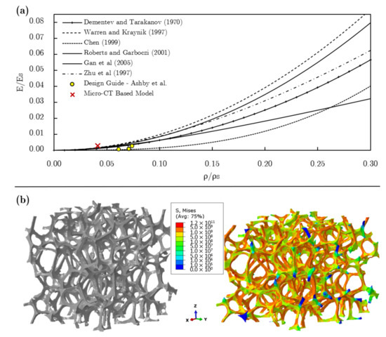
Figure 15.
(a) Relative Young’s modulus of the cubic open-cell foam specimen (Procedure 1, i.e., plain simplification), models and experimental results and (b) stress distribution (equivalent von Mises) for the cubic open-cell foam for a compression analysis.
In addition, the equivalent von Mises stress distribution along the foam can be analysed in Figure 15b. It can be noted that there are several zones where the base material’s yield stress (AlSi7Mg ≈ 150 MPa [66]) is surpassed. This happens because a random round displacement (1 mm) was imposed. Since the analysis is elastic, there is no interference in the calculation of the Young’s modulus and the stress distribution can still be analysed. The blue colour represents parts of the foam specimen where very low stresses can be found. This phenomenon originates from the definition of the boundary conditions, in which those parts are free to move, since the symmetry boundary conditions are placed on the opposite side of the model. In addition, stresses along the foam are consistent, with greater values on the struts. Some areas have a more homogeneous behaviour while others give an idea of bending.
4.4. Results Closed-Cell Foam
Figure 16 shows results obtained for each individual octant, simplified with Procedure 1, compared to several analytical models [8,51,52,54,55,56,57] and the whole foam. It is possible to observe that the sixth octant is not only the section whose behaviour most diverges from what is to be expected as well as the section which encapsulates the great majority of the large supposed artificial cracks. The rest of the parts vary a fair amount with octants one, two, three, four and five landing on the same area lower on the graph and seven and eight showing a stiffer behaviour and higher relative densities. The whole foam presents results very close to the analytical ones leaning towards the area of the less stiff octants, as is to be expected. Additionally, due to the high number of small features and cracks on the cell walls, the number of points with stress concentrations is significantly higher than if the small defects would have been removed, as in Procedure 2.
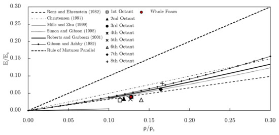
Figure 16.
Relative Young’s modulus for the closed-cell foam and the different octants for Procedure 1, i.e., plain simplification.
4.4.1. Influence of the Elimination of Defects
The presence of small defects, cracks and kinks in foams is well documented in the literature [42,43]. Their existence is known to significantly reduce the strength of foams and to be critical to their failure. However, the comparison of a model of the same foam with and without such defects is something innovative given that without the CT images it is impossible to recreate the exact same foam with such slight differences. Therefore, this analysis allows to understand how critical these small changes are.
It can be noted that Procedure 2 yielded a value of Young’s modulus significantly larger than Procedure 1, getting close to the limit imposed by the rule of mixtures (parallel) (Figure 17a). An increase was expected, given there would be more material and less kinks, but the magnitude of the difference is quite surprising. Furthermore, the difference in mass between both procedures is minimal, i.e., the two points are vertically aligned in the graph, with a difference of just 0.1% the original weight. From this information, it can be assumed that the small defects have a severe impact on the strength of the material the same way a hole has a great impact on a sheet of metal. In addition, Procedure 2 makes the mesh smoother (with less irregularities) which could lead to a better response to the applied load. The same effect can be observed for the smaller octants. In this case, two of the three tested octants show a great increase in the Young’s modulus, while one remains somewhat the same. This phenomenon might indicate that this part of the foam doesn’t have as many cracks or that their position is not as critical as in the others.
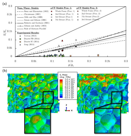
Figure 17.
(a) Relative Young’s modulus for the closed-cell foam specimen and some of its octants prepared with Procedure 1 (defects) and Procedure 2 (no defects), numerical and theoretical models and experimental results. (b) Stress distribution (Equivalent von Mises) for the same specimen during a compression analysis. Procedure 1 (plain simplification) on the left and Procedure 2 (no defects) on the right.
The foam versions with no defects had few or no points with stress concentrations while their defected counterparts presented some kinks in those regions. Figure 17b shows the stress distribution in the whole foam (equivalent von Mises stress). The yield stress is again passed because of the round imposed displacement (1 mm). The load appears to be mainly transmitted by the face walls and somewhat also by the struts. As mentioned before, the areas with small structural imperfections show a higher concentration of stresses. Moreover, the same foam simplified with the two procedures presents a distinct stress distribution, which provides some insight on the effect of the structural imperfections. The distribution appears to change significantly, demonstrating their great impact.
In Figure 17a, the models of the whole foams obtained with the procedures based on CT scans are also shown in comparison to the experimental results obtained by Duarte et al. [43] (one large foam block, FB, and four integral-skin cubes, IC), Jang et al. [67] (ALPORAS) and Triawan et al. [68] (ALPORAS). Among each other, the ALPORAS show a stiffer behaviour when compared to the foams analysed by Duarte et al., which highlights the impact of the different processes on the final results [43]. In general, both the analytical models as well as the approach described here appear to overestimate the Young’s modulus, which can derive from the lack of defects. Nevertheless, Procedure 1 comes close to what was demonstrated by the real foams emphasizing the importance of considering the small defects in the cell’s walls. Procedure 2, despite being more stable, overshoots the expected values provided by the experimental results and the models.
4.4.2. Influence of the Closing Morphological Operation
Now, the impact of the closing operation applied to the 2D slices on the Young’s modulus is studied (Figure 18). It can be observed that, for smaller radii, the impact on the Young’s modulus is small and can, therefore, be beneficial. On the contrary, for higher radii the modulus is seriously altered. This is possibly caused by some defects in the cell walls being fixed, reinforcing the structure. It is difficult to judge whether this might be a good application for this operation as it increases the values which are being examined, but, at the same time, facilitates the process and makes it more stable during simulation, i.e., less kinks and small features. It should be noted that the values discussed here are purely used as an example and for this specific foam specimen. Due to the principles of morphological operations, foams with different pore sizes and porosities will certainly require different radii in order to observe the same results.
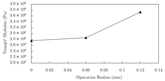
Figure 18.
Analysis of the Young’s Modulus with respect to the radius of the closing operation for the closed-cell foam specimen.
4.5. Representative Volume Element Models
An alternative to the proposed procedures based on CT scans is using Representative Volume Element (RVE) models which try to recreate the different foams with a simplified structure which can be periodically repeated to construct foams of different sizes [53,61,69]. For this reason, they are far less detailed, but simpler and require less processing power, a feature that is highly desirable in case the results are accurate. Due to being simpler also means there are no kinks and defects which can alter the results as seen with Procedures 1 and 2.
Analysing Figure 19a, it can be observed that for closed-cell foams, the predictions of the RVEs are very similar to the predictions given by the theoretical and numerical models. Consequently, they overestimate the relative stiffness of the evaluated specimen processed with Procedure 1 (with defects) and are below the results for Procedure 2 (no defects). As it can be seen in Figure 17a, the real foams present values of Young’s modulus which are lower than what is indicated by the several models and, for this reason, also lower than the ones provided by the RVEs. Then, it is possible to conclude that the first procedure elaborated and described here shows better results. Yet, the processing power required is much greater and the difficulty is higher, which can make the Representative Volume Element models one of the preferred options when it comes to mimicking and simulating closed-cell foams. Nevertheless, using CT imaging can most likely yield more accurate results for individual foams if the user is very attentive to the changes caused by the process of obtaining the 3D models from the 2D slices in the cell structure.
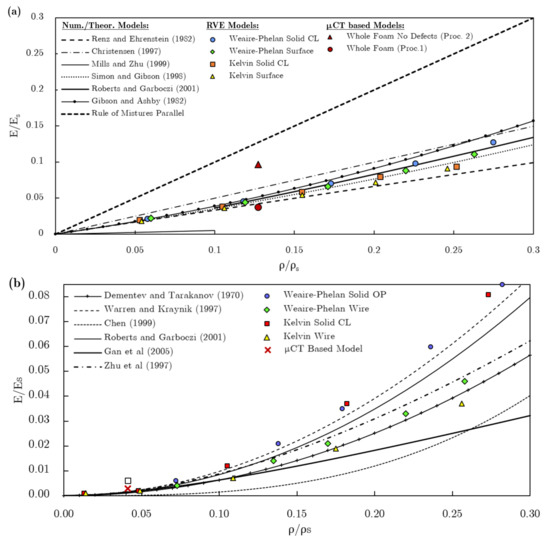
Figure 19.
Relative Young’s modulus of CT based models and RVE models for the (a) closed-cell foam specimen and (b) the cubic open-cell foam specimen.
The same tendency is observed for the open-cell foams (Figure 19b), but with greater accuracy. The Representative Volume Element models perform very well when compared to the theoretical and numerical models as well as the experimental results discussed in Figure 15a [53,69]. Again, the CT model created here shows a value of relative Young’s modulus just slightly above the predicted ones, consequently, demonstrating that it might be unnecessary to use such complex techniques. Even though this type of foam is simpler when compared to the closed-cell foam CT based model, it still is more complex and time consuming than simply using the RVEs. For this reason, the best solution might be using a RVE based model when such applications are necessary. In the end, it seems that using the CT for such purposes isn’t useful unless a more in-depth analysis is required.
4.6. Anisotropy Analysis
The two types of cells were also studied in the other two main directions allowing for an anisotropy analysis. The results are presented in Table 4 as
Table 4.
Values of Young’s modulus (Pa) and Poisson’s ratio in all three directions for the closed-cell foam specimen with both procedures and for the cubic open-cell foam specimen.
Results show that there is a high orientation dependence for all specimens. The closed-cell foam specimen simplified with Procedure 1 demonstrates a stiffer behaviour in the y direction and a high variability in Poisson’s ratios, which range from 0.25 to 0.29. Interestingly, the elimination of the small structural imperfections with Procedure 2 significantly increases the Young’s modulus in all directions and makes the specimen stiffer in the x direction, displaying, again, the strong influence of the small defects. There is also a noticeable change in the Poisson’s ratios, which range from 0.20 to 0.25. The cubic open-cell foam exhibits the largest difference, in proportion, between its Young’s moduli. In the case of the Poisson’s ratios, and are 0.56 and 0.58, which are unexpected values for open-cell foams, given a perfect open-cell foam has approximately a value of 0.33. The high values can be attributed to two factors: (1) the foam specimen is indeed highly anisotropic; (2) or/and there is the induction of local deformations by deformation mechanisms. The strain (deformation) was calculated with the average displacement of the nodes on the free sides of the specimens, which could have had their values emphasised by a rotation of the struts.
Both specimens can be approximated as orthotropic materials, there is a high orientation dependence and the material can be defined by nine different parameters instead of twenty one. The open-cell specimen could even be approximated as transversely isotropic material. The condition of anisotropy is confirmed, because of the symmetry of the stiffness matrix, by the relation [70]
where .
Figure 20 represents the 3D anisotropy maps for the closed-cell foam specimen with Procedure 1, the closed-cell foam specimen with Procedure 2 and the cubic open-cell foam specimen. The oblong shapes of the maps demonstrate the orientation dependence of the materials, therefore, the anisotropy.
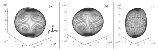
Figure 20.
3D anisotropy maps for (a) the closed-cell foam specimen with Procedure 1, (b) the closed-cell foam specimen with Procedure 2 and (c) the cubic open-cell foam specimen.
5. Conclusions
This work demonstrates that CT is an effective technique to obtain the complex geometrical and topological features of open-cell and closed-cell foams, which are otherwise difficult to capture, and use them, successfully, in simulation software. The obtained models allow for the observation of the local structure, behaviour and anisotropy, requiring high computational power when compared to other models. Therefore, high detail corresponds to slower analyses, making other simpler types of models better for other applications, for example, Representative Volume Elements (RVE).
Here, it was shown that the process from the 2D slices to the FEM model has a great impact on the results, which should be taken into consideration when developing models based on CT scans. Different types of thresholding techniques yielded different results, in terms of total mass and microstructure, therefore, the threshold was selected manually using the mass/volume as a quality indicator to guarantee the preservation of the amount of matter for finite element analyses. Results demonstrated that this process achieved very good separation between the foreground and the background and the masses/volumes of the foams were matched with differences of 0.141%, 0.138% and 0.108% of the original values for the cubic open-cell, cylindrical open-cell and closed-cell foam specimens, respectively. In contrast, the Otsu thresholding technique yielded a threshold of 70 for the closed-cell specimen (comparing to 47 for manual selection), which results in a volume/mass error of 15.408%, and the Mean-C technique a variation of 32.877% (with a radius of 2 and a constant of 5, for example). Therefore, the manual selection was preferred. In addition, the threshold was demonstrated to depend on the scan parameters and the application of the closing morphological operation shows good smoothing of the cell walls and closure of small pores, but it requires a compensation of the threshold to minimize the error in mass.
The application of reconstruction algorithms also induces some error. The two different tested reconstruction algorithms yielded very different results. The Double-Time Cubes (DTC) algorithm showed better smoothing than the Marching Cubes 33 (MC33), however, only the MC33 maintained the mass of the specimen unchanged (variations lower than 0.168%). Moreover, the smoothing caused by DTC was automatic, not allowing any control over the final result.
The two developed simplification procedures were shown to be able to obtain an STL model ready for FEM analyses. Procedure 1 maintained all small defects and cracks in the cell walls and Procedure 2 eliminated them using the discrete curvature of those features. In the end, the procedures managed to maintain the mass with small variations of a maximum of 2% of the initial volumes/masses for both types of foams (open-/closed-cell), showing also a very small difference of 0.1% between the two procedures applied to the closed-cell foam. In addition, the variation in the shape was tested with the Hausdorff algorithm and difference between meshes. Results show that the shape of the foam specimens suffered small changes even for reductions of 99% of the number of faces, i.e., values inferior to 0.04%. The quality of the mesh, described by the closeness of the triangular faces to an equilateral triangle, was improved by the Taubin smooth algorithm, while preserving the shape and mass.
The FEM meshing of the STL models was shown to be limited in most common software. For that reason, Gmsh was used, which managed to create a 3D meshes based on the surface/boundary meshes in STL. The creation of the volumetric meshes was shown to limited by the initial boundary meshes, making the development of high quality STLs very important.
In the case of the open-cell specimen, the developed model based on CT showed results very close to not only the different analytical and numerical modes but also the experimental results and the results based on RVE models. Additionally, it showed anisotropic behaviour. The closed-cell foam was tested for the two procedures (defects and no defects). The results were very positive for Procedure 1 (with defects), showing a relative Young’s modulus very close to the prediction of the analytical, numerical and RVE models and experimental results, but with some kinks and concentration of stresses in smaller features. Procedure 2 (no defects) exhibited less kinks, however, the value of relative Young’s modulus was almost double the one obtained with Procedure 1, deviating more from the several models, despite the small difference in mass between the two procedures (0.1%). This is an important finding, since it provides insight about the presence of small cracks and defects on the cell walls. They appear to substantially weaken the foam and the effect of the process of obtaining the foam models on the models themselves comes into questioning. Therefore, higher standardization might be required in order to compare this sort of numerical results with results by other authors. Moreover, the obtained results might bring awareness to cellular metal producers regarding the detrimental impact of small imperfections in the overall mechanical performance of their products. Lastly, the closing operation was verified to impact the Young’s modulus severely for larger radii. However, for smaller radii it provides smoother models with less kinks and lower increases to the Young’s modulus.
Author Contributions
Conceptualization, I.D. and J.D.-d.-O.; methodology, D.H., I.D. and J.D.-d.-O.; software, D.H.; validation, D.H., I.D. and J.D.-d.-O.; formal analysis, D.H., I.D. and J.D.-d.-O.; investigation, D.H., I.D. and J.D.-d.-O.; data curation, D.H., I.D. and J.D.-d.-O.; writing—original draft preparation, D.H.; writing—review and editing, I.D. and J.D.-d.-O.; supervision, I.D. and J.D.-d.-O. All authors have read and agreed to the published version of the manuscript.
Funding
This research was funded by Portuguese Science Foundation (FCT): UIDP/00481/2020-FCT and SFRH/BD/111515/2015, and Centro Portugal Regional Operational Program (Centro2020), under the PORTUGAL 2020 Partnership Agreement, through the European Regional Development Fund: CENTRO-01-0145-FEDER-022083.
Institutional Review Board Statement
Not applicable.
Informed Consent Statement
Not applicable.
Data Availability Statement
The raw/processed data required to reproduce these findings cannot be shared at this time as the data also forms part of an ongoing study.
Acknowledgments
This work was supported by the projects UIDB/00481/2020 and UIDP/00481/ 2020—FCT—Fundação para a Ciência e a Tecnologia; and CENTRO-01-0145-FEDER-022083—Centro Portugal Regional Operational Programme (Centro2020), under the PORTUGAL 2020 Partnership Agreement, through the European Regional Development Fund.
Conflicts of Interest
The authors declare no conflict of interest.
Abbreviations
The following abbreviations are used in this manuscript:
| CT | X-ray microcomputed tomography |
| OC | Open-Cell |
| CC | Closed-Cell |
| ROI | Region of Interest |
| VOI | Volume of Interest |
| AT | Adaptive/local Thresholding |
| MC33 | Marching Cubes 33 |
| DTC | Double-Time Cubes |
| FEM | Finite Element Method |
| FEA | Finite Element Analysis |
| NURBS | Non-uniform rational basis spline |
| STL | Standard Triangle Language file format |
| SID | Symmetry boundary conditions with an Imposed Displacement |
| SPF | Symmetry boundary conditions with a Prescribed Force |
| IC | Integral-skin Cube |
| FB | Foam Block |
| RVE | Representative Volume Element |
References
- Banhart, J.; Seeliger, H.W. Aluminium foam sandwich panels: Manufacture, metallurgy and applications. Adv. Eng. Mater. 2008, 10, 793–802. [Google Scholar] [CrossRef]
- Vesenjak, M.; Duarte, I.; Baumeister, J.; Göhler, H.; Krstulović-Opara, L.; Ren, Z. Bending performance evaluation of aluminium alloy tubes filled with different cellular metal cores. Compos. Struct. 2020, 234, 111748. [Google Scholar] [CrossRef]
- Duarte, I.; Krstulović-Opara, L.; Vesenjak, M. Axial crush behaviour of the aluminium alloy in-situ foam filled tubes with very low wall thickness. Compos. Struct. 2018, 192, 184–192. [Google Scholar] [CrossRef]
- García-Moreno, F. Commercial applications of metal foams: Their properties and production. Materials 2016, 9, 85. [Google Scholar] [CrossRef]
- Nakajima, H. Fabrication, properties and application of porous metals with directional pores. Prog. Mater. Sci. 2007, 52, 1091–1173. [Google Scholar] [CrossRef]
- Banhart, J.; Baumeister, J.; Weber, M. Powder Metallurgical Technology for the Production of Metallic Foams. In Proceedings of the European Conference on Advanced PM Materials (PM’95), Birmingham, UK, 23–25 October 1995; European Powder Metallurgy Association: Shrewsbury, UK, 1995; pp. 201–208. [Google Scholar]
- Lehmhus, D.; Vesenjak, M.; de Schampheleire, S.; Fiedler, T. From stochastic foam to designed structure: Balancing cost and performance of cellular metals. Materials 2017, 10, 922. [Google Scholar] [CrossRef]
- Gibson, L.J.; Ashby, M.F. Cellular Solids: Structure and Properties, 2nd ed.; Cambridge University Press: Cambridge, UK, 1997; pp. 1–510. [Google Scholar] [CrossRef]
- Heitor, D. Mechanical Behaviour of Aluminium Alloy Foams Modelled with X-ray Microcomputed Tomography. Master’s Thesis, University of Aveiro, Aveiro, Portugal, 2021. [Google Scholar]
- Kak, A.C.; Slaney, M.; Wang, G. Principles of Computerized Tomographic Imaging. Med. Phys. 2002, 29, 107. [Google Scholar] [CrossRef]
- Sharma, V.; Zivic, F.; Grujovic, N.; Babcsan, N.; Babcsan, J. Numerical modeling and experimental behavior of closed-cell aluminum foam fabricated by the gas blowing method under compressive loading. Materials 2019, 12, 1582. [Google Scholar] [CrossRef]
- Chaturvedi, A.; Bhatkar, S.; Sarkar, P.S.; Chaturvedi, S.; Gupta, M.K. 3D geometric modeling of aluminum based foam using micro computed tomography technique. Mater. Today Proc. 2019, 18, 4151–4156. [Google Scholar] [CrossRef]
- Kozma, I.; Zsoldos, I. CT-based tests and finite element simulation for failure analysis of syntactic foams. Eng. Fail. Anal. 2019, 104, 371–378. [Google Scholar] [CrossRef]
- Ghazi, A.; Berke, P.; Tiago, C.; Massart, T.J. Computed tomography based modelling of the behaviour of closed cell metallic foams using a shell approximation. Mater. Des. 2020, 194, 108866. [Google Scholar] [CrossRef]
- Hangai, Y.; Yamaguchi, R.; Takahashi, S.; Utsunomiya, T.; Kuwazuru, O.; Yoshikawa, N. Deformation behavior estimation of aluminum foam by X-ray CT image-based finite element analysis. Metall. Mater. Trans. A Phys. Metall. Mater. Sci. 2013, 44, 1880–1886. [Google Scholar] [CrossRef]
- Miedzińska, D.; Niezgoda, T.; Gieleta, R. Numerical and experimental aluminum foam microstructure testing with the use of computed tomography. Comput. Mater. Sci. 2012, 64, 90–95. [Google Scholar] [CrossRef]
- Veyhl, C.; Belova, I.V.; Murch, G.E.; Fiedler, T. Finite element analysis of the mechanical properties of cellular aluminium based on micro-computed tomography. Mater. Sci. Eng. A 2011, 528, 4550–4555. [Google Scholar] [CrossRef]
- Chen, Y.; Das, R.; Battley, M. Finite element analysis of the compressive and shear responses of structural foams using computed tomography. Compos. Struct. 2017, 159, 784–799. [Google Scholar] [CrossRef]
- Landis, E.N.; Keane, D.T. X-ray microtomography. Mater. Charact. 2010, 61, 1305–1316. [Google Scholar] [CrossRef]
- Viot, P.; Plougonven, E.; Bernard, D. Microtomography on polypropylene foam under dynamic loading: 3D analysis of bead morphology evolution. Compos. Part A Appl. Sci. Manuf. 2008, 39, 1266–1281. [Google Scholar] [CrossRef]
- Appoloni, C.; Fernandes, C.; Innocentini, M.; Macedo, Á. Ceramic foams porous microstructure characterization by X-ray microtomography. Mater. Res. 2004, 7, 557–564. [Google Scholar] [CrossRef]
- Burger, W.; Burge, M.J. Digital Image Processing An Algorithmic Introduction Using Java, 2nd ed.; Texts in Computer Science; Springer: London, UK, 2016. [Google Scholar] [CrossRef]
- Zhang, J.; Yan, C.H.; Chui, C.K.; Ong, S.H. Fast segmentation of bone in CT images using 3D adaptive thresholding. Comput. Biol. Med. 2010, 40, 231–236. [Google Scholar] [CrossRef]
- Otsu, N. A Threshold Selection Method from Gray-Level Histograms. IEEE Trans. Syst. Man Cybern. 1979, 9, 62–66. [Google Scholar] [CrossRef]
- Leszczyński, B.; Gancarczyk, A.; Wróbel, A.; Pia̧tek, M.; Łojewska, J.; Kołodziej, A.; Pȩdrys, R. Global and Local Thresholding Methods Applied to X-ray Microtomographic Analysis of Metallic Foams. J. Nondestruct. Eval. 2016, 35, 1–9. [Google Scholar] [CrossRef]
- Huang, D.Y.; Wang, C.H. Optimal multi-level thresholding using a two-stage Otsu optimization approach. Pattern Recognit. Lett. 2009, 30, 275–284. [Google Scholar] [CrossRef]
- Lorensen, W.E.; Cline, H.E. Marching cubes: A high resolution 3D surface construction algorithm. In Proceedings of the 14th Annual Conference on Computer Graphics and Interactive Techniques, SIGGRAPH 1987, Anaheim, CA, USA, 27–31 July 1987; pp. 163–169. [Google Scholar] [CrossRef]
- Chernyaev, E. Marching Cubes 33: Construction of Topologically Correct Isosurfaces; Technical Report; CERN CN 95-17; CERN: Saint-Petersburg, Russia, 1995. [Google Scholar]
- Bruker. Manual for Bruker-microCT CT-Analyser v.1.13; Bruker microCT: Kontich, Belgium, 2013. [Google Scholar]
- Cignoni, P.; Callieri, M.; Corsini, M.; Dellepiane, M.; Ganovelli, F.; Ranzuglia, G. MeshLab: An open-source mesh processing tool. In Proceedings of the 6th Eurographics Italian Chapter Conference, Salerno, Italy, 2–4 July 2008; pp. 129–136. [Google Scholar]
- Hoppe, H. New quadric metric for simplifying meshes with appearance attributes. In Proceedings of the IEEE Visualization Conference, San Francisco, CA, USA, 24–29 October 1999; pp. 59–66. [Google Scholar] [CrossRef]
- Garland, M.; Heckbert, P.S. Surface simplification using quadric error metrics. In Proceedings of the 24th Annual Conference on Computer Graphics and Interactive Techniques, SIGGRAPH ’97, Los Angeles, CA, USA, 3–8 August 1997; pp. 209–216. [Google Scholar] [CrossRef]
- Rossignac, J.; Borrel, P. Multi-resolution 3D approximations for rendering complex scenes. In Modeling in Computer Graphics; Springer: Berlin/Heidelberg, Germany, 1993; pp. 455–465. [Google Scholar] [CrossRef]
- Schroeder, W.J.; Zarge, J.A.; Lorensen, W.E. Decimation of triangle meshes. In Proceedings of the 19th Annual Conference on Computer graphics and Interactive Techniques—SIGGRAPH ’92, Chicago, IL, USA, 26–31 July 1992; Association for Computing Machinery (ACM): New York, NY, USA, 1992; pp. 65–70. [Google Scholar] [CrossRef]
- Taubin, G. Signal processing approach to fair surface design. In Proceedings of the ACM SIGGRAPH Conference on Computer Graphics, Los Angeles, CA, USA, 6–11 August 1995; pp. 351–358. [Google Scholar] [CrossRef]
- Taubin, G. Curve and surface smoothing without shrinkage. In Proceedings of the IEEE International Conference on Computer Vision, Cambridge, MA, USA, 20–23 June 1995; pp. 852–857. [Google Scholar] [CrossRef]
- Remacle, J.F.; Geuzaine, C.; Compère, G.; Marchandise, E. High-quality surface remeshing using harmonic maps. Int. J. Numer. Methods Eng. 2010, 83, 403–425. [Google Scholar] [CrossRef]
- Leong, K.F.; Chua, C.K.; Ng, Y.M. A study of stereolithography file errors and repair. Part 1. Generic solution. Int. J. Adv. Manuf. Technol. 1996, 12, 407–414. [Google Scholar] [CrossRef]
- Leong, K.F.; Chua, C.K.; Ng, Y.M. A study of stereolithography file errors and repair. Part 2. Special cases. Int. J. Adv. Manuf. Technol. 1996, 12, 415–422. [Google Scholar] [CrossRef]
- Meyer, M.; Desbrun, M.; Schröder, P.; Barr, A.H. Discrete Differential-Geometry Operators for Triangulated 2-Manifolds. In Visualization and Mathematics III; Springer: Berlin/Heidelberg, Germany, 2003; pp. 35–37. [Google Scholar] [CrossRef]
- Borouchaki, H.; Frey, P.J. Simplification of surface mesh using Hausdorff envelope. Comput. Methods Appl. Mech. Eng. 2005, 194, 4864–4884. [Google Scholar] [CrossRef]
- Saadatfar, M.; Garcia-Moreno, F.; Hutzler, S.; Sheppard, A.P.; Knackstedt, M.A.; Banhart, J.; Weaire, D. Imaging of metallic foams using X-ray micro-CT. Colloids Surf. A Physicochem. Eng. Asp. 2009, 344, 107–112. [Google Scholar] [CrossRef]
- Duarte, I.; Vesenjak, M.; Krstulović-Opara, L. Variation of Quasi-static and Dynamic Compressive Properties in Single Aluminium-alloy Foam Block. Procedia Mater. Sci. 2014, 4, 157–162. [Google Scholar] [CrossRef]
- Cignoni, P.; Rocchini, C.; Scopigno, R. Metro: Measuring Error on Simplified Surfaces. Comput. Graph. Forum 1998, 17, 167–174. [Google Scholar] [CrossRef]
- Dement’ev, A.G.; Tarakanov, O.G. Effect of cellular structure on the mechanical properties of plastic foams. Polym. Mech. 1970, 6, 519–525. [Google Scholar] [CrossRef]
- Warren, W.E.; Kraynik, A.M. Linear elastic behavior of a low-density kelvin foam with open cells. J. Appl. Mech. Trans. ASME 1997, 64, 787–794. [Google Scholar] [CrossRef]
- Zhu, H.X.; Knott, J.F.; Mills, N.J. Analysis of the elastic properties of open-cell foams with tetrakaidecahedral cells. J. Mech. Phys. Solids 1997, 45, 319–325. [Google Scholar] [CrossRef]
- Chen, C.; Lu, T.J.; Fleck, N.A. Effect of imperfections on the yielding of two-dimensional foams. J. Mech. Phys. Solids 1999, 47, 2235–2272. [Google Scholar] [CrossRef]
- Roberts, A.P.; Garboczi, E.J. Elastic moduli of model random three-dimensional closed-cell cellular solids. Acta Mater. 2001, 49, 189–197. [Google Scholar] [CrossRef]
- Gan, Y.X.; Chen, C.; Shen, Y.P. Three-dimensional modeling of the mechanical property of linearly elastic open cell foams. Int. J. Solids Struct. 2005, 42, 6628–6642. [Google Scholar] [CrossRef]
- Voigt, W. Ueber die Beziehung zwischen den beiden Elasticitätsconstanten isotroper Körper. Ann. Der Phys. 1889, 274, 573–587. [Google Scholar] [CrossRef]
- Reuss, A. Berechnung der Fließgrenze von Mischkristallen auf Grund der Plastizitätsbedingung für Einkristalle. ZAMM Z. Angew. Math. Mech. 1929, 9, 49–58. [Google Scholar] [CrossRef]
- Aquino, J.; Duarte, I.; Dias de Oliveira, J. Modelling and effective properties prediction of metal foams. Sci. Technol. Mater. 2018, 30, 43–49. [Google Scholar] [CrossRef]
- Renz, R.; Ehrenstein, G.W. Calculation of deformation of cellular plastics by applying the finite element method. Cell. Polym. 1982, 1, 5–13. [Google Scholar]
- Christensen, R.M. Mechanics of low density materials. J. Mech. Phys. Solids 1986, 34, 563–578. [Google Scholar] [CrossRef]
- Christensen, R.M. Mechanics of cellular and other low-density materials. Int. J. Solids Struct. 2000, 37, 93–104. [Google Scholar] [CrossRef]
- Mills, N.J.; Zhu, H.X. The high strain compression of closed-cell polymer foams. J. Mech. Phys. Solids 1999, 47, 669–695. [Google Scholar] [CrossRef]
- Piegl, L. On NURBS: A Survey. IEEE Comput. Graph. Appl. 1991, 11, 55–71. [Google Scholar] [CrossRef]
- Geuzaine, C.; Remacle, J.F. Gmsh: A 3-D finite element mesh generator with built-in pre- and post-processing facilities. Int. J. Numer. Methods Eng. 2009, 79, 1309–1331. [Google Scholar] [CrossRef]
- Marchandise, E.; Compère, G.; Willemet, M.; Bricteux, G.; Geuzaine, C.; Remacle, J.F. Quality meshing based on STL triangulations for biomedical simulations. Int. J. Numer. Methods Biomed. Eng. 2010, 26, 876–889. [Google Scholar] [CrossRef]
- Aquino, J. Methods for the Prediction of Effective Properties of Metal Foams. Master’s Thesis, University of Aveiro, Aveiro, Portugal, 2016. [Google Scholar]
- Bohm, H.J. A Short Introduction to Basic Aspects of Continuum Micromechanics; ILSB Report/ILSB-Arbeitsbericht 206 (supersedes CDL–FMD Report 3–1998); ILSB Vienna University of Technology: Vienna, Austria, 2008. [Google Scholar]
- Kirca, M.; Gül, A.; Ekinci, E.; Yardim, F.; Mugan, A. Computational modeling of micro-cellular carbon foams. Finite Elem. Anal. Des. 2007, 44, 45–52. [Google Scholar] [CrossRef]
- Rizzo, A.R. Estimating Errors in FE Analyses. Mech. Eng. CIME 1991, 113, 61–63. [Google Scholar]
- Ashby, M.; Evans, A.; Fleck, N.; Gibson, L.; Hutchinson, J.; Wadley, H.; Delale, F. Metal Foams: A Design Guide. Appl. Mech. Rev. 2001, 54, B105–B106. [Google Scholar] [CrossRef]
- Stena Aluminium. Alloy Specification. Available online: https://www.stenaaluminium.com/aluminium-alloys-and-services/alloy-specifications/ (accessed on 12 May 2021).
- Jang, W.Y.; Hsieh, W.Y.; Miao, C.C.; Yen, Y.C. Microstructure and mechanical properties of ALPORAS closed-cell aluminium foam. Mater. Charact. 2015, 107, 228–238. [Google Scholar] [CrossRef]
- Triawan, F.; Kishimoto, K.; Adachi, T.; Inaba, K.; Nakamura, T.; Hashimura, T. The elastic behavior of aluminum alloy foam under uniaxial loading and bending conditions. Acta Mater. 2012, 60, 3084–3093. [Google Scholar] [CrossRef]
- Daxner, T.; Bitsche, R.; Böhm, H.J. Space-Filling Polyhedra as Mechanical Models for Solidified Dry Foams. Mater. Trans. 2006, 47, 2213–2218. [Google Scholar] [CrossRef]
- Dowling, N. Mechanical Behavior of Materials—Engineering Methods for Deformation, Fracture and Fatigue, 4th ed.; Pearson Education: Boston, MA, USA, 2012. [Google Scholar]


Publisher’s Note: MDPI stays neutral with regard to jurisdictional claims in published maps and institutional affiliations. |
© 2021 by the authors. Licensee MDPI, Basel, Switzerland. This article is an open access article distributed under the terms and conditions of the Creative Commons Attribution (CC BY) license (https://creativecommons.org/licenses/by/4.0/).