Research on Automated Defect Classification Based on Visual Sensing and Convolutional Neural Network-Support Vector Machine for GTA-Assisted Droplet Deposition Manufacturing Process

Abstract

This paper proposes a novel metal additive manufacturing process, which is a composition of gas tungsten arc (GTA) and droplet deposition manufacturing (DDM). Due to complex physical metallurgical processes involved, such as droplet impact, spreading, surface pre-melting, etc., defects, including lack of fusion, overflow and discontinuity of deposited layers always occur. To assure the quality of GTA-assisted DDM-ed parts, online monitoring based on visual sensing has been implemented. The current study also focuses on automated defect classification to avoid low efficiency and bias of manual recognition by the way of convolutional neural network-support vector machine (CNN-SVM). The best accuracy of 98.9%, with an execution time of about 12 milliseconds to handle an image, proved our model can be enough to use in real-time feedback control of the process.

1. Introduction

Additive manufacturing (AM) is revolutionary compared to traditional processing methods in creating complex 3D-shaped components. Among the different additive manufacturing techniques, wire and arc additive manufacturing (WAAM), which combines an electric arc as heat source and wire as the feedstock material, is suitable to produce large metallic parts owing to the high deposition rates being significantly larger than powder as the feedstock [1]. Gas metal arc (GMA), gas tungsten arc (GTA) and plasma arc (PA) are the most used processes in WAAM. They all need external filler materials and a high energy-density arc heat source under an inert shielding gas [2]. Comparing with wires as feedstock, we developed a new metal additive manufacturing process in this paper, which uses fused droplets as feedstock combined with variable-polarity GTA to form aluminum alloy. The solid cylindrical aluminum alloy is inductively heated in a graphite crucible to a molten state. At the same time, a certain argon pressure is applied to make the fused aluminum alloy droplets flow out of the nozzle and fall into the molten pool by GTA. The deposited layer is formed after the liquid metal solidification. Figure 1 shows the schematic diagrams of the two different processes, where Figure 1a is the schematic diagram of WAAM, and Figure 1b is the schematic diagram of the process we presented.

The GTA process is accompanied by a highly non-linear heat source, and there are several input parameters to consider, such as the welding voltage and current, the process speed, the shielding gas flow and the type of materials [3,4]. To make the process relatively stable and restrain defects to form a good shape, non-destructive testing (NDT) plays a vital role in implementing online monitoring without changing or damaging the nature and structure of the parts. Therefore, it is economical in different levels of development and maintenance [5].

In the past few years, several typical NDT techniques such as computerized tomography (CT), radiographic testing (RT), ultrasonic testing (UT), magnetic particle inspection (MPI) and eddy current testing (ET) have been applied to the field of metal AM [6]. Chabot et al. [7] applied a phased array ultrasonic testing (PAUT) to WAAM components. With the help of X-ray radiography, the PAUT method finished defect size detection from 0.6 to 1 mm for aluminum alloy parts. Bento et al. [8] developed an eddy current testing (ECT) system where the customized ECT probes were able to locate artificial defects: at depths up to 5 mm; with a thickness as small as 350 μm; with the probe up to 5 mm away from the inspected sample surface. Wu et al. [9] used an infrared monochrome pyrometer (IMP) for accurately identifying simulated cracks on the surface of a laser metal deposition (LMD) sample. To detect lack-of-fusion defects, Montazeri et al. [10] captured the dynamic phenomena around the melt pool region by a spectrometer and an optical camera during directed energy deposition (DED). Chang et al. [11] proposed a method based on the position information of electron beam speckle to realize the three-dimensional reconstruction of the surface of the deposited parts in the process of electron beam freeform fabrication (EBF3).

As a very important method of NDT, a visual sensing system is widely used in online monitoring of metal AM. In addition, a lot of image processing algorithms suitable for different processes have been designed in order to improve the detection stability of systems. Zhuang et al. [12] proposed k-nearest neighbor (KNN) classification algorithms based on contour curve-KNN (CC-KNN) and locality preserving projection-KNN (LPP-KNN) effectively performed in vision and spectral analysis. Yu et al. [13] established the visual sensing system to capture every frame of the molten pool images matched for the actual weld location in the GMA AM process. A back propagation (BP) neural network was used to extract the shape and location features of the molten pool. Xia et al. [14] developed a visual sensing system working with a robot and a cold metal transfer (CMT) welder. The adaptive Wiener filter and the Canny algorithm were utilized to obtain information in welding pool images. Aminzadeh et al. [15] developed and trained a statistical Bayesian classifier to classify the quality of the build that signifies the defective or unacceptable build layers during laser powder bed fusion (LPBF).

Deep learning (DL) algorithms have recently grabbed the attention of scientists due to their strong ability to learn high-level features from raw data, and in most cases, they are much better than traditional algorithms in terms of accuracy and robustness. Convolutional neural networks (CNN) are particularly more used in computer vision tasks which include image classification, object detection, segmentation and so on [16,17,18,19]. However, restricted by the computation performance and datasets, CNN fell out of use for several years until AlexNet was proposed by Krizhevsky for the ImageNet competition in 2012 [20,21]. Subsequently, VGGNet [22] and GoogleNet [23] were proposed considering the width and depth of the network respectively. ResNet [24] proved that the depth of the network can be increased very deeply. With the rise of state-of-the-art CNN architectures, researchers have introduced them to the field of metal AM. Cui et al. [25] used the Missouri S&T dataset (optical microscope images of LMD parts) to train and investigate Hyper-parameters including kernel size and the number of layers of their CNN model. Kwon et al. [26] applied CNN to melt-pool images with respect to six laser power labels in selective laser melting (SLM). The classification failure rate was under 0.01. Yin et al. [27] adopted CNN to analyze the welding process parameters and the weld dimensions from twin-wire CMT welding of 5083 aluminum alloy. Zhang et al. [28] presented the application of deep learning framework for automated surface quality inspection in recognition of under-melt, beautiful-weld and over-melt categories in LPBF. The classification accuracy of the finally developed model on the UB-Moog dataset is 0.82 by optimizing hyper parameters. Wang et al. [29], based on previous work [13], developed a prediction network (PredNet) to predict the change of molten pool shape 140ms in advance. Through regression network (SERes), the predicted results were regressed to the accurate weld reinforcement information of the deposited layer in advance. Tomaz et al. [30] realized multi-objective optimization during the GTAW process with the help of an artificial neural network (ANN) and a genetic algorithm (GA). The optimal welding parameters, including welding current = 222 A, welding speed = 25 cm/min, nozzle deflection distance = 8 mm, travel angle = 25°, were determined, and the determination coefficient (R2) and RMSE value of all response parameters were satisfactory, and the R2 of all the data remained higher than 0.65.

The theorem called “No Free Lunch” states that no algorithm can perform well on all problems, so the objective of this work is to explore a good CNN-SVM-based model with the best possible optimizer function, good learning rate and a varied number of epochs to identify the common defects with best accuracy in GTA-assisted DDM. The results can be used for quasi-real-time (layer-wise) process control, further process decisions or corrective actions.

The remainder of this paper is organized as follows. In Section 2, we introduce the GTA-assisted DDM experiment platform and the CNN-SVM architecture in detail. In Section 3, the hyperparameters optimization is introduced in detail, including performance evaluation and the visualization of CNN features. The conclusion is summarized in Section 4.

2. Experiment Platform and Methods

2.1. Experiment Platform

GTA-assisted DDM experiment platform combined the GTAW platform (Fronius, Pettenbach, Austria), melting type high frequency induction heating equipment (SPG50K-15AB, ShuangPing Power Technology Co., Ltd., ShenZhen, China) and a visual sensing system (Mikrotron GmbH, Unterschleissheim, Germany ), which are shown in Figure 2. The GTA welding platform included a welding power supply (Fronius Magicwave 3000 Job G/F, Fronius, Pettenbach, Austria) and a TIG robot welding torch (TBi RT20, TBi Industries GmbH, Fernwald-Steinbach, Germany). The melted aluminum 2024 was processed into a cylinder with a diameter of 60 mm, height of 80 mm and put in the graphite crucible. Aluminum 2024 grade was selected as work material because it is high-strength duralumin and extensively used in high-load parts such as skeletons and skins on aircraft. The chemical composition of that is shown in

Table 1. The chemical composition of melted material (wt.%).

Elements	Cu	Mn	Mg	Zn	Al
Composition	4.75	0.5	1.56	0.25	Others

. The size of the substrate was 220 mm × 220 mm × 10 mm and a 65° inclination angle formed between the welding torch and the substrate. The visual sensing system consisted of a CMOS camera (EoSens CL: CAMMC1362, Mikrotron GmbH, Unterschleissheim, Germany) with an optical lens (AT-X 100 mm F2.8, Kenko Tokina Co., Ltd., Tokyo, Japan), an image acquisition card (Xtium-CL MX4, Teledyne DALSA, Waterloo, ON, Canada) and other data storage devices. The high-speed camera was fixed on a tripod (Benro IF28+) and focused on the back edge of the deposition layer through the glass panel on the front of the glovebox. Once focused by adjusting the aperture to the maximum position, the aperture and the camera exposure time were adjusted at the same time to darken the field of view on the monitor. During the experiment, the droplets falling into the molten pool accurately matched each frame of image to a specific welding position.

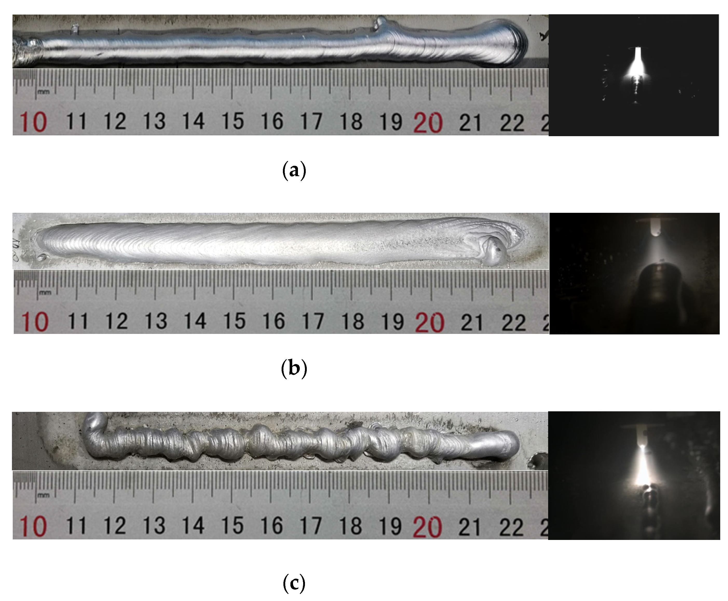
2.2. Experiment Methods

GTA-assisted DDM was mainly affected by parameters such as forming speed (Ts), forming current (Ip), forming flux (Qv), substrate temperature (Tb), etc. The overall dimensions of a good Al-2024 single-pass deposited layer were generally stable, and the surface of the deposited layer had fish-scale patterns, as shown in Figure 3c. It can be seen that the deposited layer spreads continuously and is metallurgically bonded well to the substrate. Figure 3a shows the cross section of the deposited layer.

Table 2. Standard baseline process parameters.

Current	Forming Flux	Substrate Temp	Travel Speed	Shield Gas Flux
260 A	140 mm3/s	280 °C	8 mm/s	15 L/min

lists the welding parameters as a standard baseline to achieve good processing conditions. Images of good Al-2024 single-pass deposited layers were captured and recorded, then several defects were introduced by altering process parameters one at a time. Finally, morphology images of defective deposited layers were also recorded.

Defects like lack of fusion between the deposited layer and the substrate mean that overflow and discontinuity of the deposited layer are prone to appear when process parameters change. Lack of fusion is mainly caused by insufficient heat input. When Ip ≤ 200 A or Tb ≤ 220 °C, it is difficult to spread the deposited layer and bond with the substrate poorly. Overflow is mainly due to excessive heat input and forming flux, when Ip ≥ 280 A or Qv ≥ 200 mm³/s, the heat accumulation is serious and the molten droplets cannot be completely absorbed by the molten pool. Discontinuity is mainly caused by the excessive forming speed, when Ts ≥ 30 mm/s, the droplets will not fall into the molten pool continuously, causing fluctuations in the outer dimensions of the deposited layer. Figure 4. shows the macroscopic morphology and raw captured images with a size of 1280 × 1024 pixels for the above three common defects at different process parameters, which provided enough information about the defects.

2.3. Preprocessing

The size of raw captured images (1280 × 1024 pixels) had an approximate size of 1.2 MB for each one, which contained a substantial number of black pixels surrounding the deposited layer and the welding arc as seen in Figure 4. As a result of the hardware constraints, during the training stage of the algorithms, where the model receiving a higher resolution requires significantly more GPU memory. The subsampling operation is necessary before creating the deep learning dataset [31]. The reliability and speed of the algorithms are improved by region of interest (ROI) segmentation, histogram equalization and image filtering [32]. Figure 5 shows four types of data after ROI segmentation. The segmented images with 326 × 495 pixels were compressed to 155 kB to 160 kB. There were “good” (582), “lack of fusion” (641), “overflow” (589) and “discontinuity” (588). Among them, data at the beginning or end of the process that seriously affected the sample were given up to minimize the impact of sample imbalance on performance of algorithms.

2.4. Data Augmentation

Generally speaking, parameters of many deep CNN architectures are in the millions; a lot of data was required to make these parameters work correctly for training. It does not work to rely on new data completely in AM because of time and economic costs [33]. Data augmentation needs to be used to improve the model generalization ability due to the high diversity of welding conditions [34]. In this paper, scaling as well as translation, rotation, flipping, adding “Salt and Pepper” noise and changing the lighting condition was applied to create more data to make the algorithms have a better generalization effect. The result of the original image “good” processed by the above data augmentation methods was shown in Figure 6. Where scaling was achieved by three scale factors of 0.9, 0.75, 0.6, translation was done by moving 20% left, right, up and down respectively and rotation was finished by sequentially rotating 6° once a time from −30° to 30°. The number of each class after data augmentation was given in

Table 3. The number of images in each category.

	Good	Lack of Fusion	Overflow	Discontinuity	Total
Train	6984	8136	7212	7056	29,388
Test	2328	2712	2404	2352	9796

and they were split into two main subsets: training and testing, with approximatively 75% and 25%, respectively.

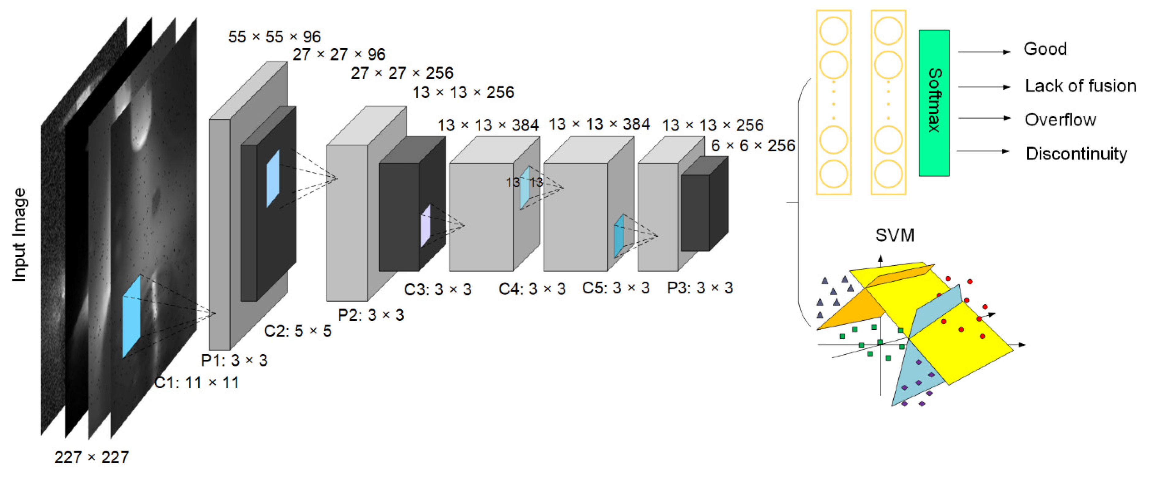
2.5. CNN+SVM Architecture

CNN consists of multiple, repeating components which are stacked in layers: convolution, pooling, fully connected and classifier layers. Among them, local receptive field, shared weights and pooling are the three most important concepts [19,20]. The model in this paper draws on the ideas of the classic AlexNet model and linear SVM. The overall structure is composed of two parts: feature extraction and classification, which is shown in Figure 7.

The feature extraction consists of five convolutional layers named C1–C5 with a size of corresponding filters: 11 × 11, 5 × 5, 3 × 3 respectively and three maximum pooling layers named P1–P3. It can be described as follows:

$$x^l=f(b^l+{\displaystyle \sum _j^J{\displaystyle \sum _i^I{w}_{i.j}^l{x}_{i,j}^{l-1}}})$$

(1)

$$f(x)=\mathrm{Re}\mathrm{LU}(x)=\{\begin{array}{c}x\\ 0.01x\end{array}\begin{array}{c}x>0\\ x\le 0\end{array}$$

(2)

$$a_j=\underset{N\times N}{\max }(a_i^{N\times N}u(n,n))$$

(3)

where (J, I) denotes the size of the filters, J is the height of the filters, and I is the width of the filters. b^l denotes the bias of the convolutional layer. x^l−1 denotes the output of the previous layer. w^l denotes the weight of the convolutional layer. f(x) is the nonlinear activation function rectified linear units (ReLU) shown as Equation (2). Pooling operations are shown as Equation (3), which is a form of non-linear down-sampling and used to replace the output of a certain location with a summary statistic of nearby [34,35]. Finally, batch normalization was used for centering and normalization of the images and applied before the fully connected layers instead of local response normalization (LRN) for its unobvious regularization effects.

It comes to the classification stage. On the one hand, output of P3 was flattened to transfer to the fully connected layers with a 0.4 dropout to prevent overfitting of the data. The was model constructed here with the better choice of optimizer function between stochastic gradient descent (SGD) and adaptive moment estimation (Adam). Varied learning rates ranging from 1 × 10⁻³ to 1 × 10⁻⁵ were selected and optimized by minimizing cross-entropy loss function. That can be described as:

$$H(p,q)=-{\displaystyle \sum _{x}p(x)\log q(x)}$$

(4)

where H is the cross entropy, which can determine how close the actual output is to the expected output, p is the expected output of sample x and logq(x) is the logarithm of the actual output of sample x.

On the other hand, the top layer is replaced by a linear SVM (L2-SVM), which minimizes the squared hinge loss, shown as Equation (5). Output of the pooling layer, M3, is given to the SVM algorithm and the classification performs.

$$\underset{w}{\min }\frac{1}{2}{w}^{T}w+C{\displaystyle \sum _{n=1}^{N}Max{(1-w^T{x}_n{t}_n,0)}^2}$$

(5)

where w is the normal vector of classification hyperplane, C is a regularization parameter, x_n is the feature vector, t_n is the label it belongs to.

The overall training procedure was performed on a PC with an Intel Core i5-4570 CPU, RAM of 12 GB, a NVIDIA RTX 2080 Ti GPU, running Windows 10 professional with CUDA 9.0 libraries. The software environment was Python 3.6 using TensorFlow 1.13.1.

2.6. Evaluation Metrics

The commonly used evaluation metrics were described as Equations (6)–(9):

$$Accuracy=(TP+TN)/(TP+TN+FP+FN)$$

(6)

$$Precision=TP/(TP+FP)$$

(7)

$$Recall=TP/(FN+TP)$$

(8)

$$Fscore=(2\times Precision\times Recall)/(Precision+Recall)$$

(9)

Among them, accuracy is defined as the number of correct predictions, precision refers to how many of all positive samples are correctly identified, also called positive predictive value (PPV), recall is a measure of the degree of discrimination of all positive samples, which tells how many samples judged as positive are true. F score indicates the overall performance of the precision and recall, which is the harmonic mean of precision and recall. True Positive (TP) describes the number when the true value is positive and the model is considered to be positive; True Negative (TN) counts the number when the true value is negative and the model is considered to be negative; False Positive (FP) illustrates the number when the true value is negative but the model is considered to be positive; False Negative (FN) represents the number when the true value is positive but the model is considered to be negative.

3. Results and Discussion

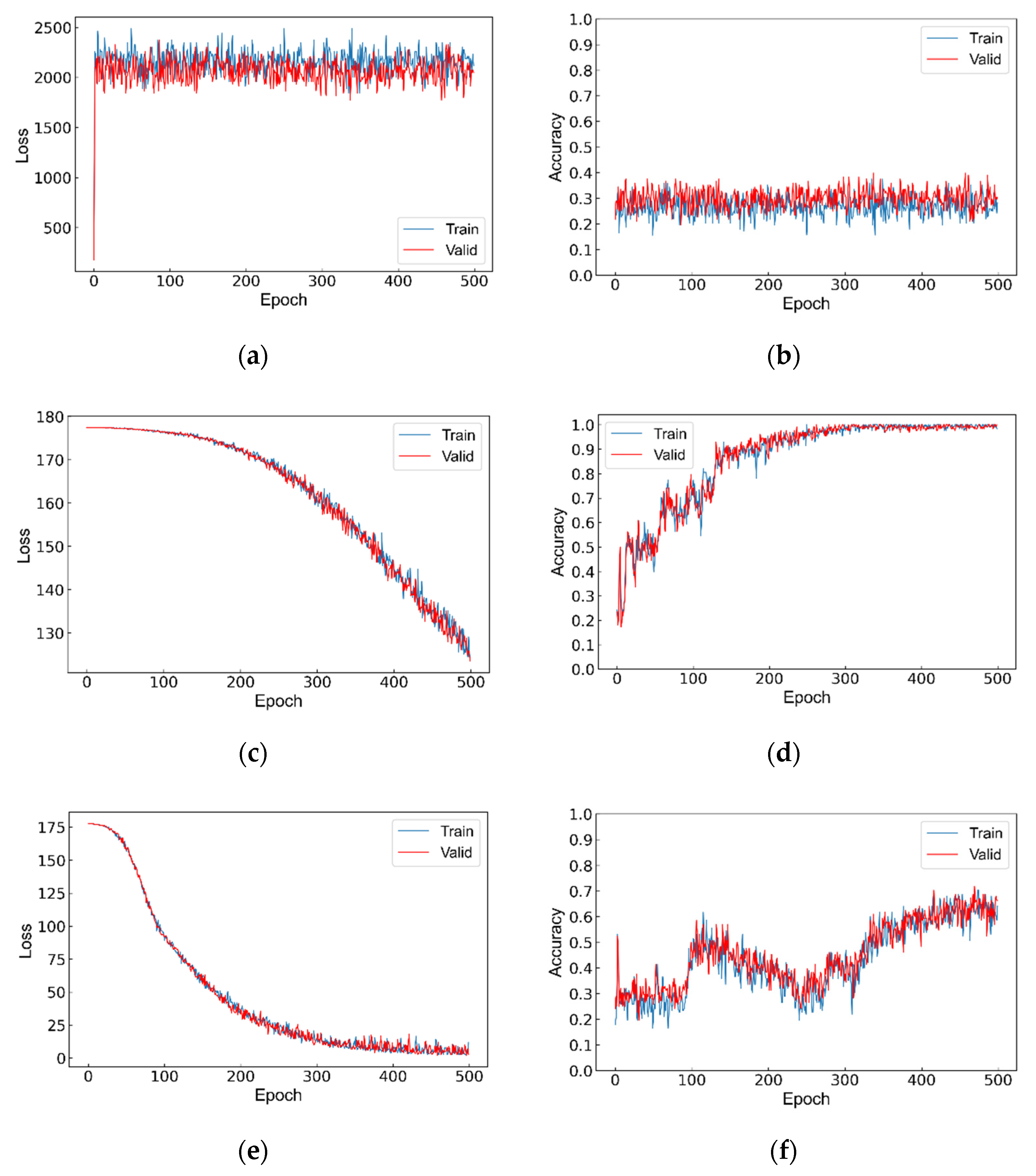
3.1. Tuning of CNN Architecture

The classic AlexNet model has more than 60 million parameters and more than 650,000 neurons. If the parameter adjustment is not ideal, the performance will not be represented well. Batch size, learning rate, epochs, weight initialization, dropout, the choice of optimizer and data normalization are several indicators we are mainly concerned about. Figure 8 shows the effect of a varied batch size on the stability of model convergence, which presents loss and accuracy after training 500 epochs. A larger batch size is conducive to more stable model convergence but constrained by hardware. Hence, the maximum batch size used in our model is 128. It is particularly emphasized that networks can converge unless the weight initialization of the fully connected is 1 × 10⁻⁴. The weights of other layers can be initialized using a Gaussian distribution with a mean value of 0 and a standard deviation of 0.01 or 0.1. The neuron bias of all layers is initialized to a constant 0.1.

The change-of-learning rate is often combined with the optimization function used in model training. This study compared two different optimization functions of SGD and Adam [36,37], and then analyzes the impact of learning rate on model convergence. SGD randomly selects a point for calculating the fastest descent direction instead of traversing the entire training data set. This can greatly speed up the iteration speed while taking the local optimal solution into account. It can be described as:

$$J(\theta )=\frac{1}{2}{\displaystyle \sum _{i=1}^m{(y^i-h_{\theta }(x^i))}^2}$$

(10)

$${\theta }_j^{\text{'}}={\theta }_j+\alpha (y^i-h_{\theta }(x^i))x_j^i$$

(11)

where, J(θ) is the loss function that needs to be minimized, m is the sample batches, h_θ(x^j) is the function of parameter θ fitting to the sample, α is called learning rate.

The Adam algorithm calculates step size to be updated by calculating the first moment estimation and second moment estimation of the gradient, which are the mean of the gradient and the decentralized variance of the gradient, to design independent adaptive learning rates for different parameters. Figure 9 and Figure 10 show the process of training models with different learning rates and optimization functions. It can be seen that the selection of the learning rate has a great influence on whether the model converges. When the learning rate is 1 × 10⁻⁴ and Adam is used, the model converges with the highest accuracy of convergence. If the learning rate is set too large, the larger training step makes the parameters oscillate back and forth on both sides of the optimal solution. If the learning rate is too small, the convergence speed will be greatly reduced and the final model will not reach the best accuracy.

3.2. Performance Evaluation

The precision and recall of our model were evaluated on the test dataset according to evaluation metrics in Section 2.4 and the results were reported in

Table 4. Precision, recall, and F score of our model on the test dataset.

Class	Precision	Recall	F Score
Good	0.93	0.96	0.945
Lack of fusion	0.92	0.89	0.905
Overflow	0.95	0.94	0.945
Discontinuity	0.91	0.88	0.895

. Overall, F score can basically reach 0.9, indicating good classification performance. At the same time, a comparative experiment of KNN, single use of SVM or CNN and our model was carried out in order to highlight our model in terms of recognition accuracy and efficiency. The results are listed in

Table 5. Results of accuracy and time for different classification methods.

Method	Accuracy	Time (s)
KNN	0.926	0.61
SVM	0.864	0.13
CNN	0.96	0.008
Our model	0.989	0.012

. It can be seen that our model has an accuracy of 98.9% with a time of about 12 milliseconds to recognize an image, which would be enough to use in a real-time feedback control of our process.

3.3. The Visualization of CNN Features

The visualization of the feature map after convolution can help us understand what each layer of convolution has learned and show the process of abstracting features layer by layer. Figure 11 shows the feature maps of four samples representing “overflow”, “good”, “discontinuity” and “lack of fusion” after having been learned by different layers. Some feature maps focus on the background of images, others are more inclined to the outline of images. The 96 and 256 feature maps from the first two convolutional layers C1, C2 are basically about information of edges, stripes and grayscale where the shape of different classes can be seen clearly. Starting from C3, a larger number of 3 × 3 convolution kernels are used. Compared with the previous convolution layer, the 3 × 3 convolution kernel has a larger receptive field on the convolution output of this step. This expansion of the receptive field allows the convolutional layer to combine low-level features (lines, edges) into higher-level features (curves, textures) and this more abstract expression makes it less visually interpretable or difficult to differentiate.

4. Conclusions

Quality monitoring based on visual sensing was applied to a novel metal additive manufacturing process, GTA-assisted DDM, in this paper.

(1) A large number of process experiments were implemented with parameters including forming speed (Ts), forming current (Ip), forming flux (Qv) and substrate temperature (Tb) deviating from a standard baseline. Different kinds of morphology images of deposited layers were obtained: “good”, “lack of fusion”, “overflow” and “discontinuity”.

(2) Translation, rotation, flipping, adding “Salt and Pepper” noise and other data augmentation methods were used to expand the original image dataset and reduce the cost of the process experiments.

(3) Training of a CNN-SVM model based on AlexNet and linear support vector machine was completed, where a batch size of 128 and learning rate of 1e-4 on Adam function were determined as the optimal value, and the output of trained P3 as a feature was transferred to the SVM for classification. The results showed that F scores of our model could reach 0.9 mostly, and compared to KNN, or single use of SVM or CNN, it had a best test set accuracy of 98.9% as well as an execution time of about 12 milliseconds to handle an image, which provided a more sufficient control time in the GTA-assisted DDM.

References

1. Williams, S.W.; Martina, F.; Addison, A.C.; Ding, J.; Pardal, G.; Colegrove, P. Wire plus Arc Additive Manufacturing. Mater. Sci. Technol. 2016, 32, 641–647. [Google Scholar] [CrossRef] [Green Version]
2. Rodrigues, T.A.; Duarte, V.; Miranda, R.M.; Santos, T.G.; Oliveira, J.P. Current Status and Perspectives on Wire and Arc Additive Manufacturing (WAAM). Materials 2019, 12, 1121. [Google Scholar] [CrossRef] [Green Version]
3. Rodriguez-Cobo, L.; Ruiz-Lombera, R.; Conde, O.M.; Lopez-Higuera, J.M.; Cobo, A.; Mirapeix, J. Feasibility study of Hierarchical Temporal Memories applied to welding diagnostics. Sens. Actuator A Phys. 2013, 204, 58–66. [Google Scholar] [CrossRef]
4. Arora, H.; Kumar, V.; Prakash, C.; Pimenov, D.; Singh, M.; Vasudev, H.; Singh, V. Analysis of Sensitization in Austenitic Stainless Steel-Welded Joint. In Advances in Mechanical Engineering; J.B. Metzler: Jalandhar, India, 2021; pp. 13–23. [Google Scholar]
5. Gao, X.D.; Li, G.H.; Chen, Z.Q.; Lan, C.Z.; Li, Y.F.; Gao, P.P. Modeling for detecting weld defects based on magneto-optical imaging. Appl. Optics. 2018, 57, 6110–6119. [Google Scholar] [CrossRef]
6. Florence, S.E.; Samsingh, R.V.; Babureddy, V. Artificial intelligence based defect classification for weld joints. In Proceedings of the IOP Conference Series: Materials Science and Engineering, Bandung, Indonesia, 9–13 July 2018; IOP Publishing: Kattankulathur, India, 2018; Volume 402, p. 012159. [Google Scholar]
7. Chabot, A.; Laroche, N.; Carcreff, E.; Rauch, M.; Hascoet, J.Y. Towards defect monitoring for metallic additive manufacturing components using phased array ultrasonic testing. J. Intell. Manuf. 2020, 31, 1191–1201. [Google Scholar] [CrossRef]
8. Bento, J.B.; Lopez, A.; Pires, I.; Quintino, L.; Santos, T.G. Non-destructive testing for wire plus arc additive manufacturing of aluminium parts. Addit. Manuf. 2019, 29, 100782. [Google Scholar]
9. Wu, Y.; Cui, B.; Xiao, Y. Crack Detection during Laser Metal Deposition by Infrared Monochrome Pyrometer. Materials 2020, 13, 5643. [Google Scholar] [CrossRef]
10. Montazeri, M.; Nassar, A.R.; Stutzman, C.B.; Rao, P. Heterogeneous sensor-based condition monitoring in directed energy deposition. Addit. Manuf. 2019, 30, 100916. [Google Scholar] [CrossRef]
11. Chang, S.H.; Zhang, H.Y.; Xu, H.Y.; Sang, X.H.; Wang, L.; Du, D.; Chang, B.H. Online Measurement of Deposit Surface in Electron Beam Freeform Fabrication. Sensors 2019, 19, 4001. [Google Scholar] [CrossRef] [Green Version]
12. Zhao, Z.; Guo, Y.T.; Bai, L.F.; Wang, K.H.; Han, J. Quality monitoring in wire-arc additive manufacturing based on cooperative awareness of spectrum and vision. Optik 2019, 181, 351–360. [Google Scholar] [CrossRef]
13. Yu, R.W.; Zhao, Z.; Bai, L.F.; Han, J. Prediction of Weld Reinforcement Based on Vision Sensing in GMA Additive Manufacturing Process. Metals 2020, 10, 1041. [Google Scholar] [CrossRef]
14. Xia, C.Y.; Pan, Z.X.; Zhang, S.Y.; Polden, J.; Wang, L.; Li, H.J.; Xu, Y.L.; Chen, S.B. Model predictive control of layer width in wire arc additive manufacturing. J. Manuf. Process 2020, 58, 179–186. [Google Scholar] [CrossRef]
15. Aminzadeh, M.; Kurfess, T.R. Online quality inspection using Bayesian classification in powder-bed additive manufacturing from high-resolution visual camera images. J. Intell. Manuf. 2019, 30, 2505–2523. [Google Scholar] [CrossRef]
16. Tao, W.; Leu, M.C.; Yin, Z. American Sign Language alphabet recognition using Convolutional Neural Networks with multiview augmentation and inference fusion. Eng. Appl. Artif. Intell. 2018, 76, 202–213. [Google Scholar] [CrossRef]
17. Li, K.; Wu, Z.; Peng, K.-C.; Ernst, J.; Fu, Y. Tell Me Where to Look: Guided Attention Inference Network. In Proceedings of the 2018 IEEE/CVF Conference on Computer Vision and Pattern Recognition, Salt Lake City, UT, USA, 27 February 2018; pp. 9215–9223. [Google Scholar]
18. Wang, T.; Chen, Y.; Qiao, M.; Snoussi, H. A fast and robust convolutional neural network-based defect detection model in product quality control. Int. J. Adv. Manuf. Technol. 2018, 94, 3465–3471. [Google Scholar] [CrossRef]
19. Azimi, S.M.; Britz, D.; Engstler, M.; Fritz, M.; Mücklich, F. Advanced steel microstructural classification by deep learning methods. Sci. Rep. 2018, 8, 2128. [Google Scholar] [CrossRef]
20. Lecun, Y.; Bengio, Y.; Hinton, G. Deep learning. Nature 2015, 521, 436–444. [Google Scholar] [CrossRef]
21. Krizhevsky, A.; Sutskever, I.; Hinton, G.E. ImageNet classification with deep convolutional neural networks. Adv. Neural Inf. Process. Syst. 2012, 1097–1105. [Google Scholar] [CrossRef]
22. Simonyan, K.; Zisserman, A. Very deep convolutional networks for large-scale image recognition. arXiv 2014, arXiv:1409.1556. [Google Scholar]
23. Szegedy, C.; Liu, W.; Jia, Y.Q.; Sermanet, P.; Reed, S.; Anguelov, D.; Erhan, D.; Vanhoucke, V.; Rabinovich, A. Going deeper with convolutions. In Proceedings of the IEEE Conference on Computer Vision and Pattern Recognition (CVPR), Boston, MA, USA, 23–28 June 2015; pp. 1–9. [Google Scholar]
24. He, K.; Zhang, X.; Ren, S.; Sun, J. Deep Residual Learning for Image Recognition. In Proceedings of the IEEE Conference on Computer Vision and Pattern Recognition (CVPR), Las Vegas, NV, USA, 27–30 June 2016; pp. 770–778. [Google Scholar]
25. Cui, W.Y.; Zhang, Y.L.; Zhang, X.C.; Li, L.; Liou, F. Metal Additive Manufacturing Parts Inspection Using Convolutional Neural Network. Appl. Sci. 2020, 10, 545. [Google Scholar] [CrossRef] [Green Version]
26. Kwon, O.; Kim, H.G.; Ham, M.J.; Kim, W.; Kim, G.H.; Cho, J.H.; Kim, N.I.; Kim, K. A deep neural network for classification of melt-pool images in metal additive manufacturing. J. Intell. Manuf. 2020, 31, 375–386. [Google Scholar] [CrossRef]
27. Yin, L.M.; Wang, J.Z.; Hu, H.Q.; Han, S.G.; Zhang, Y.P. Prediction of weld formation in 5083 aluminum alloy by twin-wire CMT welding based on deep learning. Weld. World. 2019, 63, 947–955. [Google Scholar] [CrossRef]
28. Zhang, B.B.; Jaiswal, P.; Rai, R.; Guerrier, P.; Baggs, G. Convolutional neural network-based inspection of metal additive manufacturing parts. Rapid Prototyp. J. 2019, 25, 530–540. [Google Scholar] [CrossRef]
29. Wang, Y.M.; Zhang, C.R.; Lu, J.; Bai, L.F.; Zhao, Z.; Han, J. Weld Reinforcement Analysis Based on Long-Term Prediction of Molten Pool Image in Additive Manufacturing. IEEE Access 2020, 8, 69908–69918. [Google Scholar] [CrossRef]
30. Tomaz, I.d.V.; Colaço, F.H.G.; Sarfraz, S.; Pimenov, D.Y.; Gupta, M.K.; Pintaude, G. Investigations on quality characteristics in gas tungsten arc welding process using artificial neural network integrated with genetic algorithm. Int. J. Adv. Manuf. Technol. 2021, 1–15. [Google Scholar] [CrossRef]
31. Bacioiv, D.; Melton, G.; Papaelias, M.; Shaw, R. Automated defect classification of Aluminium 5083 TIG welding using HDR camera and neural networks. J. Manuf. Process 2019, 45, 603–613. [Google Scholar] [CrossRef]
32. Yahia, N.B.; Belhadj, T.; Brag, S.; Zghal, A. Automatic detection of welding defects using radiography with a neural approach. In Proceedings of the 11th International Conference on the Mechanical Behavior of Materials (ICM), Como, Italy, 5–9 June 2011; p. 10. [Google Scholar]
33. Gaikwad, A.; Imani, F.; Yang, H.; Reutzel, E.; Rao, P. In Situ Monitoring of Thin-Wall Build Quality in Laser Powder Bed Fusion Using Deep Learning. Smart Sustain. Manuf. Syst. 2019, 3, 98–121. [Google Scholar] [CrossRef]
34. Zhang, Z.F.; Wen, G.R.; Chen, S.B. Weld image deep learning-based on-line defects detection using convolutional neural networks for Al alloy in robotic arc welding. J. Manuf. Process. 2019, 45, 208–216. [Google Scholar] [CrossRef]
35. Zhu, H.X.; Ge, W.M.; Liu, Z.Z. Deep Learning-Based Classification of Weld Surface Defects. Appl. Sci. 2019, 9, 3312. [Google Scholar] [CrossRef] [Green Version]
36. Kingma, D.; Ba, J. Adam: A Method for Stochastic Optimization. arXiv 2014, arXiv:1412.6980. [Google Scholar]
37. Duchi, J.; Hazan, E.; Singer, Y. Adaptive Subgradient Methods for Online Learning and Stochastic Optimization. J. Mach. Learn. Res. 2011, 12, 2121–2159. [Google Scholar]
Figure 1. The schematic diagrams of wire and arc additive manufacturing (WAAM) and gas tungsten arc (GTA)-assisted droplet deposition manufacturing (DDM). (a) WAAM; (b) GTA-assisted DDM.
Metals 11 00639 g001
Figure 2. GTA-assisted DDM experiment platform. (a) Schematic diagram; (b) physical diagram.
Metals 11 00639 g002
Figure 3. Good Al-2024 single-pass deposited layer. (a) Cross-section of deposited layer; (b) Partial enlargement of deposited layer; (c) Deposited layer with good morphology.
Metals 11 00639 g003
Figure 4. The macroscopic morphology of common defects. (a) Lack of fusion (Ip ≤ 200 A or Tb ≤ 220 °C); (b) overflow (Ip ≥ 280 A or Qv ≥ 200 mm3/s); (c) discontinuity (Ts ≥ 30 mm/s).
Metals 11 00639 g004
Figure 5. Four types of data after region of interest (ROI) segmentation. “good” (582) vs. “lack of fusion” (641) vs. “overflow” (589) vs. “discontinuity” (588).
Metals 11 00639 g005
Figure 6. The result of the original image “good” processed by data augmentation. (a) the resized image of the original image “good” with a size of 224 × 224 pixels; (b) the result in the order of flipping, changing the lighting condition, adding “Salt and Pepper” noise, scaling, translation and rotation.
Metals 11 00639 g006
Figure 7. The schematic of convolutional neural network-support vector machine (CNN-SVM) model.
Metals 11 00639 g007
Figure 8. The effect of varied batch size on the stability of model convergence. (a,b) batch size = 16; (c,d) batch size = 32; (e,f) batch size = 64; (g,h) batch size = 128.
Metals 11 00639 g008
Figure 9. Using SGD to train the model with different learning rates. (a,b) learning rate = 1 × 10⁻³; (c,d) learning rate = 1 × 10⁻⁴; (e,f) learning rate = 1 × 10⁻⁵.
Metals 11 00639 g009
Figure 10. Using Adam to train the model with different learning rates. (a,b) learning rate = 1 × 10⁻³; (c,d) learning rate = 1 × 10⁻⁴; (e,f) learning rate = 1 × 10⁻⁵.
Metals 11 00639 g010
Figure 11. The feature maps of four samples representing “overflow”, “good”, “discontinuity” and “lack of fusion” after having been learned by different layers.
Metals 11 00639 g011