Article

The Concept of a Novel Path Planning Strategy for Wire + Arc Additive Manufacturing of Bulky Parts: Pixel

1
Department of Mechanic and Materials, Federal Institute of Maranhão (IFMA), Barra do Corda 65950-000, Brazil
2
Center for Research and Development of Welding Processes (Laprosolda), Federal University of Uberlandia (UFU), Uberlândia 38408-100, Brazil
3
Graduate Program in Materials Science and Engineering, Federal University of Parana (UFPR), Curitiba 80060-000, Brazil
4
Division of Welding Technology, Department of Engineering Science, Production Technology West, University West, 461 32 Trollhättan, Sweden
*
Author to whom correspondence should be addressed.
Metals 2021, 11(3), 498; https://doi.org/10.3390/met11030498
Submission received: 7 February 2021 / Revised: 15 March 2021 / Accepted: 15 March 2021 / Published: 17 March 2021
(This article belongs to the Special Issue Directed Energy Deposition of Metal Alloys)

Abstract

:
An innovative trajectory strategy was proposed and accessed for wire arc additive manufacturing (WAAM), applicable to different and more complex geometries, rather than being a single solution. This strategy, named Pixel, can be defined as a complex multitask procedure to carry out optimized path planning, whose operation is made through computational algorithms (heuristics), with accessible computational resources and tolerable computational time. The model layers are fractioned in squared grids, and a set of dots is systematically generated and distributed inside the sliced outlines, resembling pixels on a screen, over which the trajectory is planned. The Pixel strategy was based on creating trajectories from the technique travelling salesman problem (TSP). Unlike existing algorithms, the Pixel strategy uses an adapted greedy randomized adaptive search procedure (GRASP) metaheuristic, aided by four concurrent trajectory planning heuristics, developed by the authors. Interactions provide successive trajectories from randomized initial solutions (global search) and subsequent iterative improvements (local search). After all recurrent loops, a trajectory is defined and written in machine code. Computational evaluation was implemented to demonstrate the effect of each of the heuristics on the final trajectory. An experimental evaluation was eventually carried out using two different not easily printable shapes to demonstrate the practical feasibility of the proposed strategy.

1. Introduction

Wire + arc additive manufacturing (WAAM) has been drawing attention from industries and researchers around the world. High deposition rate, geometry flexibility, energy efficiency and the low initial cost of equipment and consumables are some of the attractive characteristics of this process. Based on arc welding processes, for which the technology is reasonably established, and, consequently, more acceptable by end-users, WAAM uses readily available consumables, which have been standardized and tested in the field. Notwithstanding, the trajectory planning (also known as path planning) for the deposition torch is one of the key factors for the success of this technology, although not always commented on, and sometimes even neglected. Trajectory planning, being a key factor, in turn, encompasses some complexity. The operational optimization of torch movements (in terms of building time, number of stops and restarts and overcoming of geometric obstacles) is the first function of trajectory planning. However, other roles are expected from efficient trajectory planning. According to Rodrigues et al. [1], mediocre planning may result in porosity, internal defects, lack of fusion between adjacent beads and high residual stresses. Debroy et al. [2] cited that printed piece anisotropy can be avoided and/or eliminated with good strategies for torch path.
Nonetheless, additive manufacturing trajectory is basically planned as a stack of flat slices that configure the geometry to be printed. Additive manufacturing slices can be defined as thin thickness, flat layers that are geometrically described by the top view cross-section. The layers are usually generated using slicing softwares, which basically is responsible for the conversion of a 3D object model to specific instructions for the printer. The top view cross-section of the layers delineates geometric shapes with different sizes and outline complexities. In relation to bulky parts, geometric complexity is an obstacle to be overcome. An example of printing difficulties is found in slices composed by nonconvex cross-sectional polygons, with or without obstacles (such through- or blind-holes of different shapes).
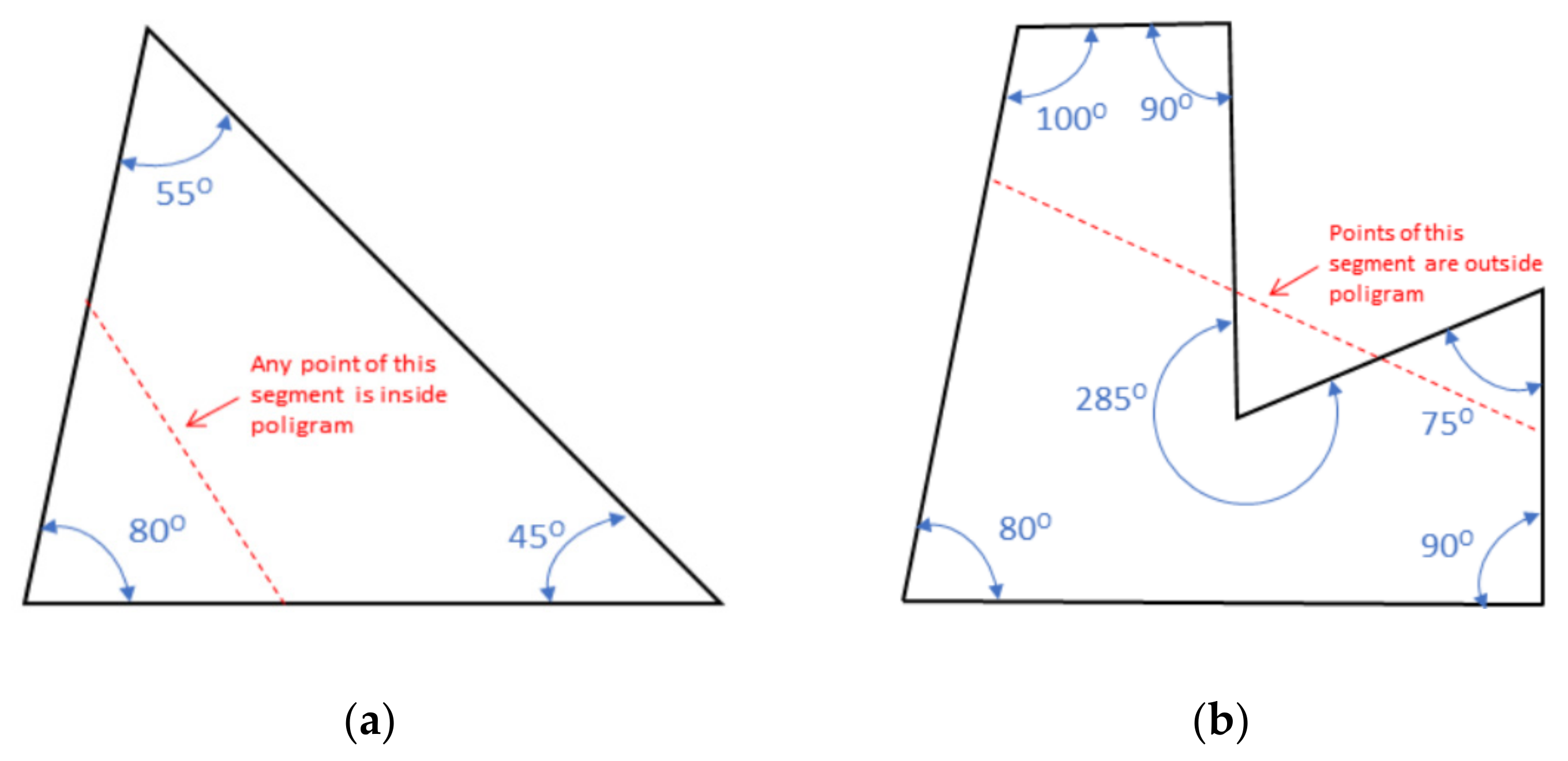
According to Gerdjikov and Wolff [3], convex polygons are those in which every internal angle is less than 180°, as illustrated in Figure 1a. Note that in the nonconvex configuration, Figure 1b, at least one internal angle is between 180° and 360°, so that points of a line segment between two points on the polygon boundary of the polygon can be located outside the polygon. In the case of nonconvex geometries, inefficient trajectories can lead to voids inside the printed part [4]. When holes are presented, “empty” trajectories (paths with no deposition) are used to avoid this obstacle; low surface quality due to geometric irregularities caused by frequent arc extinction and reignition are the consequences [5].
From current literature, there are at least three classical pattern strategies for trajectory planning applicable to WAAM, namely, raster, zigzag and contour [6,7,8]. However, due to the geometric complexities, some of these strategies have been adapted towards layer geometry simplification (polygonal division) or merged with others (hybrid trajectory planning strategies), sharing the merits of various approaches. Figure 2 illustrates examples of classical and hybrid strategies adopted by different researchers. The raster strategy is likely the most basic one (Figure 2a) and can be uni- or bi-directional. If proper parametrization is applied to the several starts and stops when raster strategy is employed, this becomes a flexible strategy. Material and heat accumulation can be eliminated by setting idle times between stops and starts. To obtain a continuous deposition per layer, an old concept used in WAAM to fill a polygon is based on a zigzagging pattern. As illustrated in Figure 2b, with a one-way movement in a given direction up to reach a polygon border, the torch, then, faces the edge of this border for a given spacing value, before inverting the trajectory direction (in cycled pattern). Wang et al. [6] claim process efficiency decay off this approach, due to arc extinctions that forcedly occur in parts with more complex geometries (such as internal holes). The likely first adaptation of the zigzag strategy carried out in WAAM was proposed several years before by Dwivedi and Kovacevic [7]. This strategy was called continuous (Figure 2c), consisting of zigzag trajectories planned to leave staggered gaps between the paths, in such a way that the gaps were sequentially closed by another zigzag trajectory in the inversed direction. It is noteworthy that the continuous strategy can be hybridlike adapted to other strategies, for example, spiral, as illustrated in Figure 2d.
Another adaptation to the zigzag strategy was proposed in Wang et al. [6] and illustrated in Figure 2e. The authors proposed a deposition trajectory strategy based on the water-pouring rule. In summary, the algorithm for deposition strategy is based on the identification of inflection points (such as nonconvex angles) in the geometry of the polygon that represents layer area (see this approach description in Figure 2e). Initially, the torch follows a zigzag pattern until an inflection point is met. Then, torch movement direction is reversed, so that the new shape (a partition of the polygon) after the inflection point is filled using the same pattern. However, a return line is planned so that the torch can escape from the bottom of the polygonal partition. The same procedure is maintained until all polygon partitions are filled.
In the contour strategy, Figure 2f,g, the arc torch follows the subsequent inscribed edges of an external polygon, through parallel displacements (pre-established offsets) relative to the polygon edges. The torch sweep can follow either parallel (2f) or spiral (2g) patterns, in either in-outward or out-inward orientation. However, in the case of parallel scanning, the transition between two edges is made by connecting its starting points, as indicated by red arrows in Figure 2f. These contour strategies are easily applied to convex polygons, but may not perform satisfactorily when it comes to nonconvex polygons. According to Ding et al. [8] and Xiong et al. [11], problems such as voids inside the parts or at very acute angled corners, and heat accumulation in the center of the workpiece (which cause residual stress and/or deformation) are recurrent in these strategies. The out-inward scanning direction is prone to generate material accumulation at the center, unless a programmed progressive adjustment of the parameters is made.
Skeletal structures (Figure 2h,i) are contour adaptation approaches to solve the limitations of nonconvex shapes. Ding et al. [8] proposed the medium axis transformation (MAT) method for solid parts (Figure 2h), with and without holes, and for thin-walled parts. Applying MAT, they skeletonized two-dimensional geometry and performed contour-like in-outward oriented sweeps. However, this method presented noncontinuous trajectories for bulky parts, with several arc stops and restarts to avoid the torch depositing beyond the polygon edges (these interruptions are emphasized by green/red circles in Figure 2h). Ding et al. [9] improved his approach and presented an adaptive medial axis transformation (A-MAT), by adapting the spacing between contours around the polygon skeleton and through re-parametrization (noticeable by gap variations between lines), resulting in continuous paths (Figure 2i).
Unlike the classical strategies presented so far, the polygon division strategy (Figure 2j) aims to reduce the complexity of nonconvex geometries by partitioning them into simpler polygons, for subsequent deposition planning, as also proposed by Dwivedi and Kovacevic [7]. According to the authors, each simple polygon is filled with one of the continuous strategies, yet in such a way that the trajectories are interconnected as a single path. However, with an increasing complexity of the initial polygon, its decomposition can result in simple but not necessarily convex polygons (see partition 2 in Figure 2j, as an example). To work around this problem, Ding et al. [10] performed a similar approach, but dividing the nonconvex polygon into only convex polygons (Figure 2k). Each sub-polygon was filled with a continuous strategy (in this case, a hybrid contour and zigzag), interconnected as a single path. Still using the same strategy, Liu et al. [4] segmented a nonconvex polygon into convex polygons to apply the contour and zigzag deposition strategy, but focusing on surfaces with corners of sharp angles, as illustrated in Figure 2l. In this strategy, a calculated displacement of the vertex of acute angles was applied to correct voids left during trajectory planning by contour strategy. However, this strategy of dividing polygons also presents difficulties when manufacturing parts with circular holes [6].
With a similar view of that described above, Wang et al. [6] cite that, although there are many strategy planning strategies, these strategies can be classified into three categories, according to their origin and evolution. The first class originated in the raster method and subsequently developed into the zigzag, continuous line and convex polygon methods. The second category originated from the contour method, which in turn developed into the medial axis transformation and adaptive medial axis transformation methods. The third category is the hybrid method that combines the advantages of these previous two categories by applying them in different regions.
In general, the strategies above mentioned (among others that can be also applied and not openly reported) were developed as solutions to solve deposition flaws in layer building for specific cases. New setbacks always appear when trying to replicate them in other geometries. In addition, there is no concern in trying an optimization of the trajectory planning (in terms of time or number of stops and restarts, for instance). In most cases they are based on a one only solution, with low path flexibilities (the flexibility is more trial and error related, mostly based on swapping from in-outward to out-inward direction in the contour strategy, or the change of the angle in the zigzag strategy, or even intercalating/bidirecting raster strategy). These remarks indicate that there is room for creating more strategies for generating trajectories for WAAM. Therefore, the objective of this work was to propose an alternative deposition strategy for WAAM, for which innovation would be its applicability in different and more complex geometries (higher flexibility), rather than being a solution for only one case. The objective extends to the use of the proposed strategy for trajectory optimization.

2. The Proposal of a Novel Strategy for WAAM Deposition: Pixel

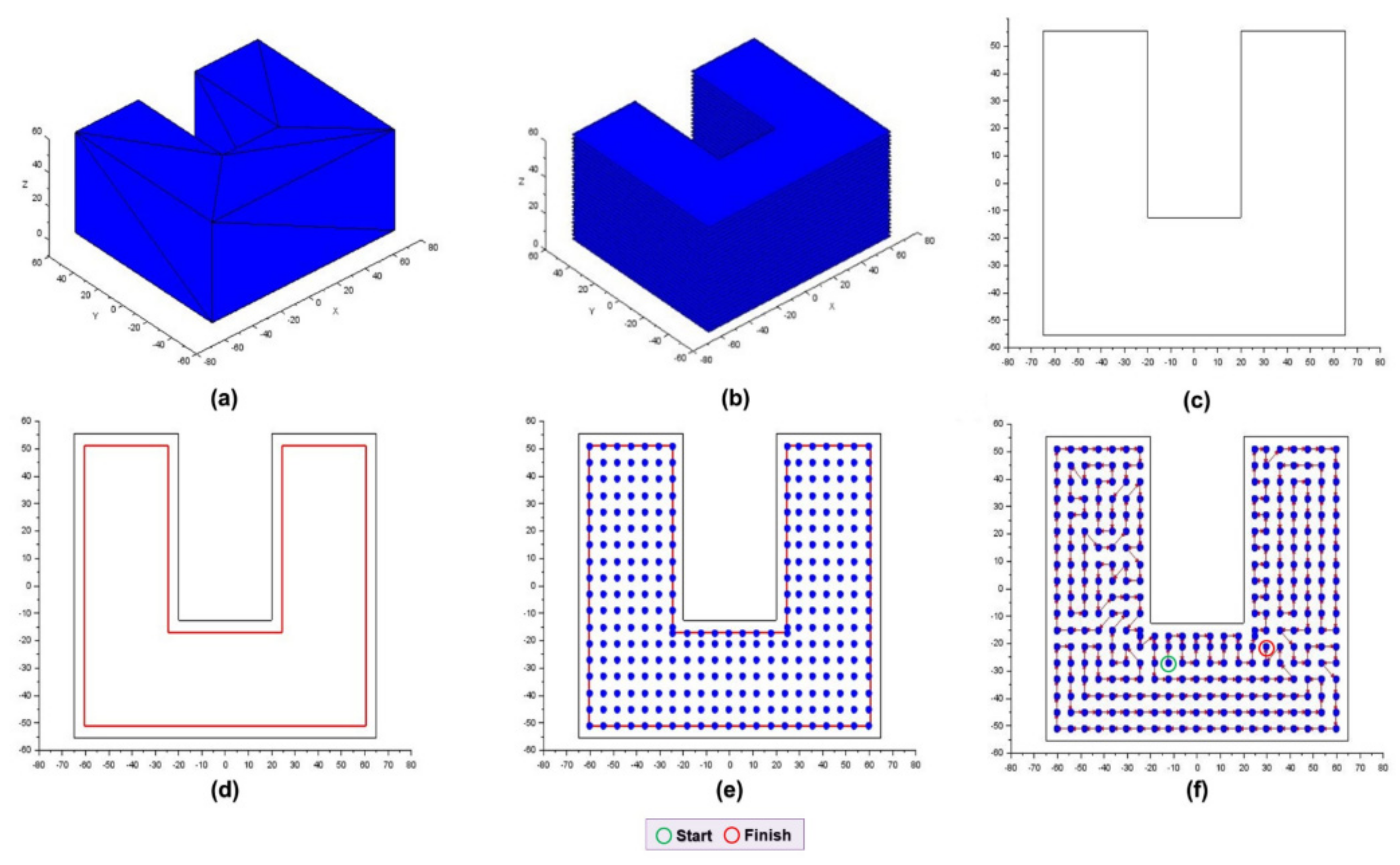
The Pixel deposition trajectory strategy to be introduced in this work can be defined as a complex multitask procedure to carry out the trajectory planning of WAAM parts. The end-user, as a nonpassive agent, is required to input the height between layers, path widths, path overlapping and number of interactions and to take the final decision on the trajectory to adopt. The operation of the procedure is made through computational algorithms (heuristics), with accessible computational resources and tolerable computational time. A heuristic, or a heuristic technique, is defined in current literature as to optimization (for instance, according to Yang [12]), as any approach aiming to find a trial and error solution that may not be optimal but is sufficient (acceptable), considering a reasonably practical timeframe. In a few words, the model layers in Pixel are fractioned in squared grids, over which the trajectory is planned. To model the problem, a set of dots is generated and distributed within the top-view cross-section outline of the slice, resembling pixels on a screen (a dot matrix to form a raster graphic, in other words, a grid composed of a collection of small squares). The useful intersections between the grid lines and the edges of the slice are hereafter referred to as nodes. The technique used in this Pixel strategy for optimization was based on creating a trajectory from a well-known route optimization named travelling salesman problem (TSP), whose challenge is to find the shortest yet most efficient route for the torch to take, given a list of specific positions. There might be other approaches for solving this problem, not yet explored in current literature on additive manufacturing. Unlike existing algorithms, the Pixel strategy uses an adapted greedy randomized adaptive search procedure (GRASP) metaheuristic to additive manufacturing. GRASP is aided by four distinct concurrent heuristics of trajectory planning, namely nearest neighbor, biased, alternate and random contour, and the 2-opt algorithm. This approach consists of iterations made up from successive constructions of randomized initial solutions (global search) and subsequent iterative improvements (local search). After all the recurrent loops, a trajectory is defined and written in machine code.
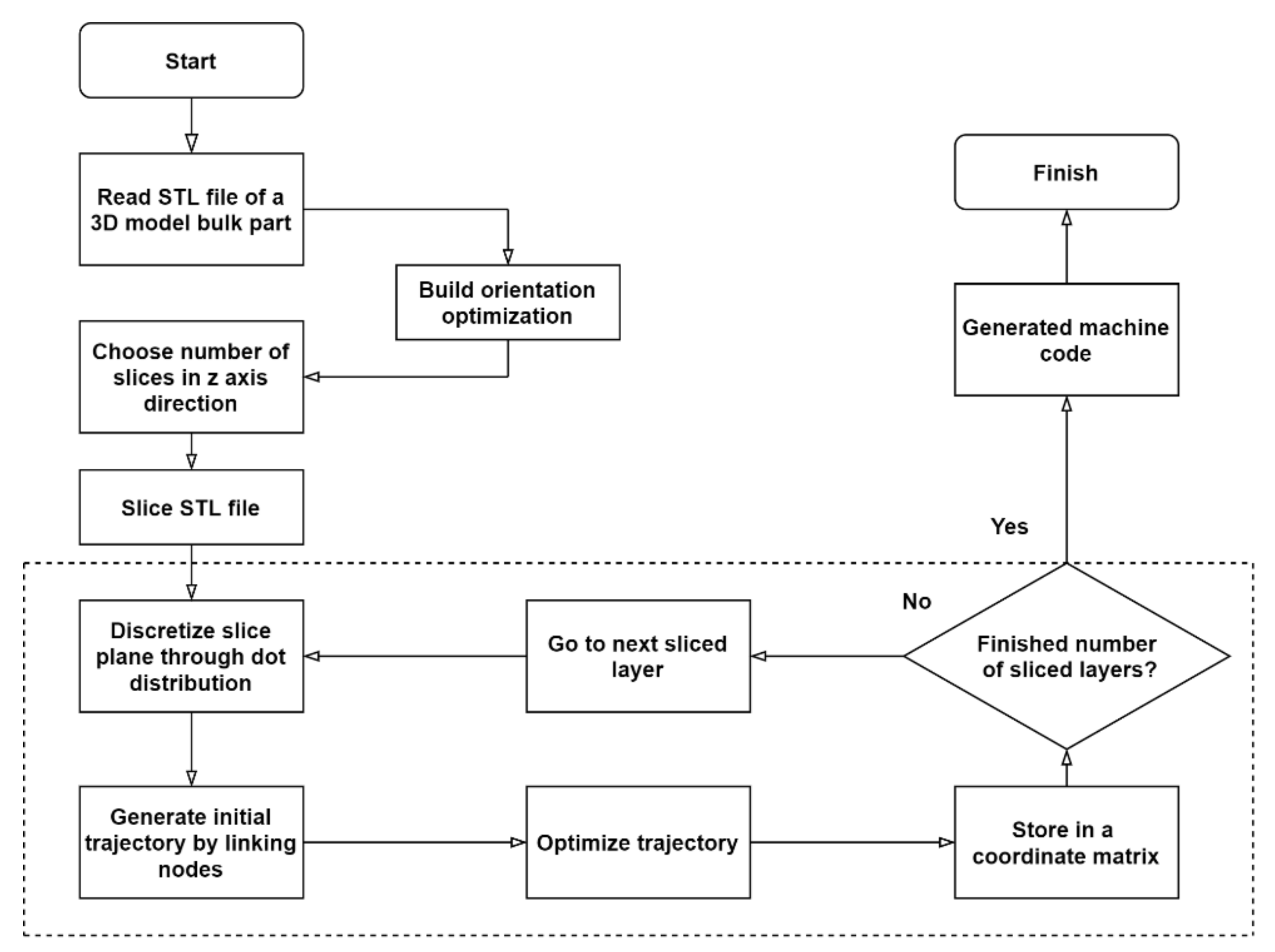
To detail the proposal, the Pixel strategy itself is flowcharted as in Figure 3. A basic process chain for WAAM begins with a 3D CAD model that is converted into an AMF or STL format file, which is accordingly sliced by dedicated software, hereafter alluded to as the “printing process planning software” (PPPS). From a PPPS is expected more than the basic functions of slicing the model and generating a machine code for the WAAM printer. In general, before machine code generation, a proper PPPS should also define the tool path (trajectory) planning. The first steps of the process, i.e., reading the STL file from the 3D model, orientation optimization and introduction of the layer heights and digital slicing of the model, are usually common to traditional, yet comprehensive, printing process planning. They will not be discussed further here, keeping the arguments concentrated on the following four steps of the proposed Pixel torch trajectory planning:
1 Discretization of the layers (through distribution of dots all over the layer surfaces, i.e., modelling the environment as a grid);
2 Starting position definition and node connections (generating an initial trajectory);
3 Trajectory Optimization (recurrent start position choices and reconnections of the nodes from the trajectory generated in the previous step, in order to obtain the shortest path to be travelled by the torch);
4 Storage of the generated optimized trajectories (to compose a set of batches of trajectories to be selected and, accordingly, supply instructions to the printing machine, in the form of coordinates in an array).
These four steps are repeated over all layers generated by the slicing process (in the case of layers with the same cross section, a trajectory generated in the initial layer can be replicated to the others). After concluding the loop, the best (according to the criterion) stored array of coordinates is converted into G code (machine code), which is sent to the WAAM printer. The entire algorithm described here has been implemented in the open-source software Scilab.

2.1. Discretization of Layers and Node Indexing

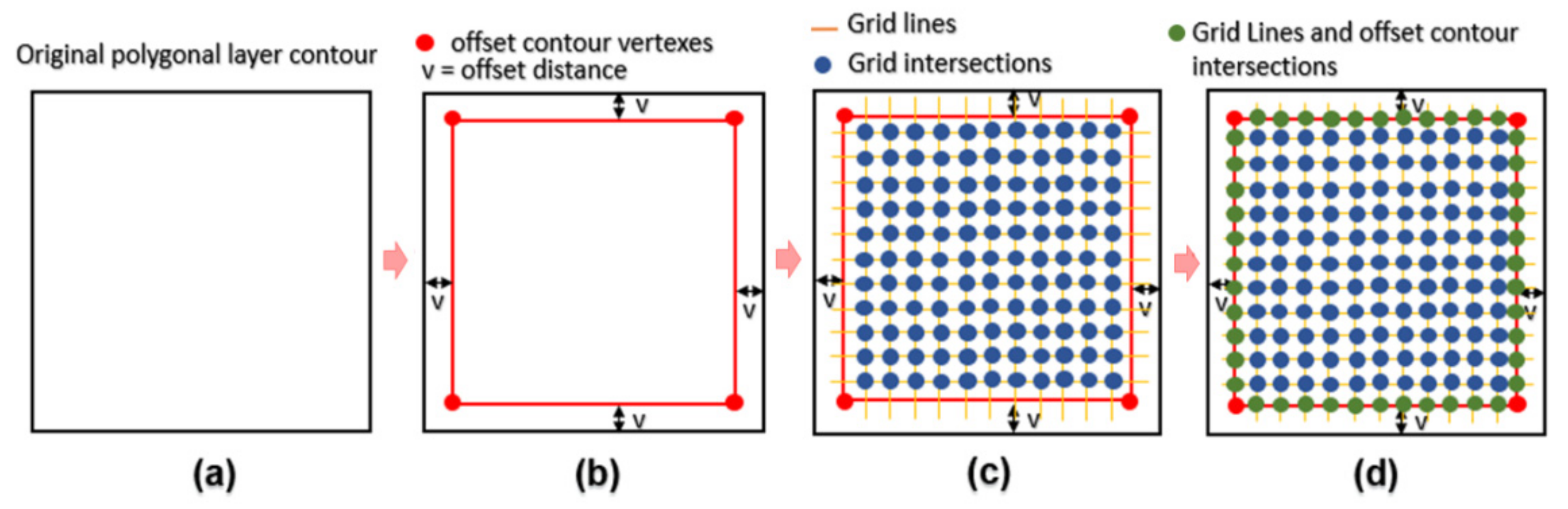
The discretization process, as proposed here, consists of four phases, that is, insertion of offset contours in the sliced layers, generation of a grid to generate dots (these two first stages are demonstrated in Figure 4), simplification of dots (as illustrated in Figure 5) and indexing of nodes (as established in Figure 6). In the first phase, the process provides a new contour to the original polygon (Figure 4a) at an offset distance from the slice edges, represented by the letter “v” in Figure 4b, composed of a simplified shape (for example purposes). From this equidistance, an internal (inscribed) surface contour is created to reduce excess or avoid material shortages at the edges of the original layer shape (for other geometries rather than that in Figure 4a, the offset would take another profile, yet keeping the same role). Then, in a second phase, equally spaced horizontal and vertical line segments (from the lower and most left positioned vertex of the offset contour) are virtually plotted over the plane, performing a grid. The intersections of these lines (blue dots in Figure 4c) and between these lines and the edges of the offset (green dots in Figure 4d) and the offset contour vertices (red dots in Figure 4b), all together form the pixel dots. It is emphasized that the spacing value is an input to the algorithm in question, to be defined by the process analyst, and should be considered as the distance between two weld beads arranged side by side (considering potential overlapping). It is therefore justified that equidistance may not be obtained at the top and right edges of the offset contour.
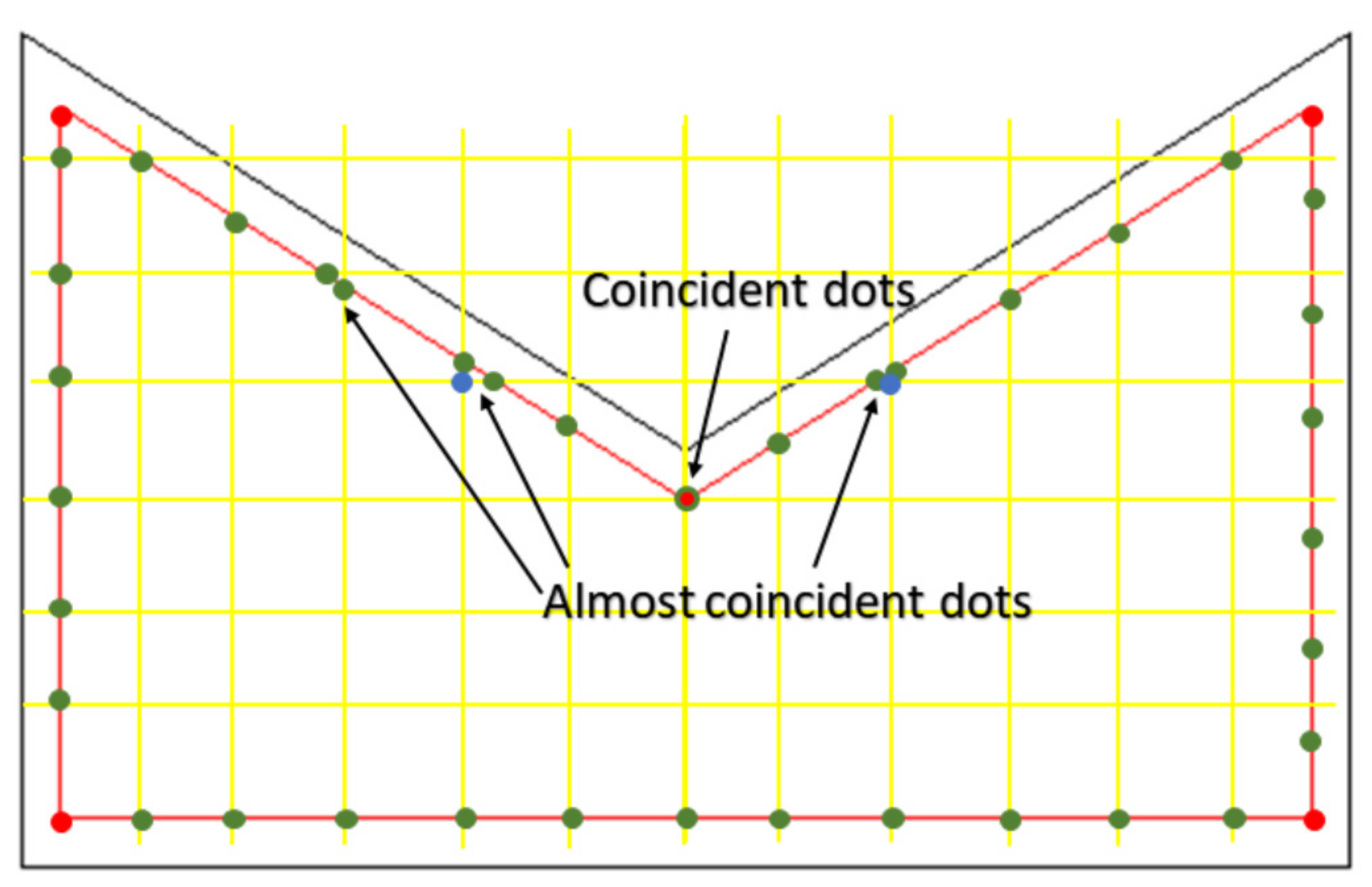
It is important to emphasize that coincident dots may arise, due to layer topology and the spacing values of the segments, as illustrated in Figure 5. In this example, the coincident dot arose because a straight segment (in yellow) of the grid crosses the offset contour (in red) at one of the vertices, which is also taken as an intersection of the discretization. There are cases where dots are coincident, or almost coincident, also highlighted in Figure 5. Therefore, a simplification of the model should be applied. Only one of these overlapping dots is considered and the others are eliminated from the discretization, which reduces the processing time to generate the trajectory. In addition, nearby dots with Euclidean distance of up to 1.0 mm are likewise removed from the model, as they will not generate significant differences during deposition. Considering the elimination of dots created during the initial discretization, the remaining dots (useful dots) are going to be referred hereafter as nodes.
Given continuity to the discretization protocol, the assigned nodes are ordered from left to right and bottom to top and, following, indexed (coded) numerically in ascending order. This indexing of each node is already illustrated in Figure 6, where i1 represents the first node of the layer (with a respective coordinate). Accordingly, the following nodes in the same horizontal row are indexed in ascending order, arranged to the right, i.e., dot in represents the last node of the first horizontal layer row and dot in+1 represents the first node of the second horizontal layer row. Hence, the indexing resumes at the second row from the first column, following the same pattern until the last dot (imax) is reached at the rightmost point of the utmost row.

2.2. Starting Position Definition and Node Connections to Define a Trajectory

The sets of nodes and their connections were modelled according to the travelling salesman problem (TSP). This approach is based on the problem of a traveling salesman who leaves an initial city and must visit all the cities programmed in a row and return to the city of departure. As a goal, he/she should plan the shortest route, however not going to a city already visited. In general, two solutions for the TSP are known. In the first, a start node is defined at random by a computer routine and a first route is generated, applying the rule of no-duplicated visits, followed by other routes improved by local search heuristics. The second solution would be to create alternative routes from different start nodes. By one means or the other (or even together), the best route is eventually provided. Aziz Ouaarab [13] and Zia et al. [14] showed the different approaches to solve the TSP in specific cases, such as railway track optimization, robot movement, vehicle routing, among others. Wasser et al. [15], in turn, successfully applied heuristic of trajectory planning in additive manufacturing of polymers.
To simulate this problem as a base for the Pixel strategy, each node (the remaining dots) created on the surface (Section 2.1) corresponds to a city of the TSP and the node connections resemble the path travelled by the salesmen, i.e., the deposition trajectory. Figure 7 is a diagrammatic representation of this problem, in which the set of interconnected nodes is represented by i1, i2, i3, …, i16, where i1i2i3 ≠… ≠ i16 for the case in which 16 is the total number of nodes of this example. Trajectory (T) is represented by a set of connections between nodes, without repetitions, where i 1 i 5 , for instance, represents an effective link between node i1 and node i5. Note that in this representation the last visited “city” (i7) and the initial visited “city” (i1) are not connected (even the first node is not visited again).
The distance between two nodes ip and iq is calculated by the vector distance between the two coordinates (ipx,ipy) and (iqx,,iqy),, as expressed in Equation (1), which represents the Euclidean distance (d).
d ( i p i q ) = i p x i q x 2 +   i p y i q y 2
The total trajectory distance (DT), the objective function, is calculated according to the summation of all connections between two nodes in T, as described in Equation (2):
D T = f = 1 n d f ( i p i q )
where n represents the total number of connections between nodes in T and f represents the indexes of each connection.
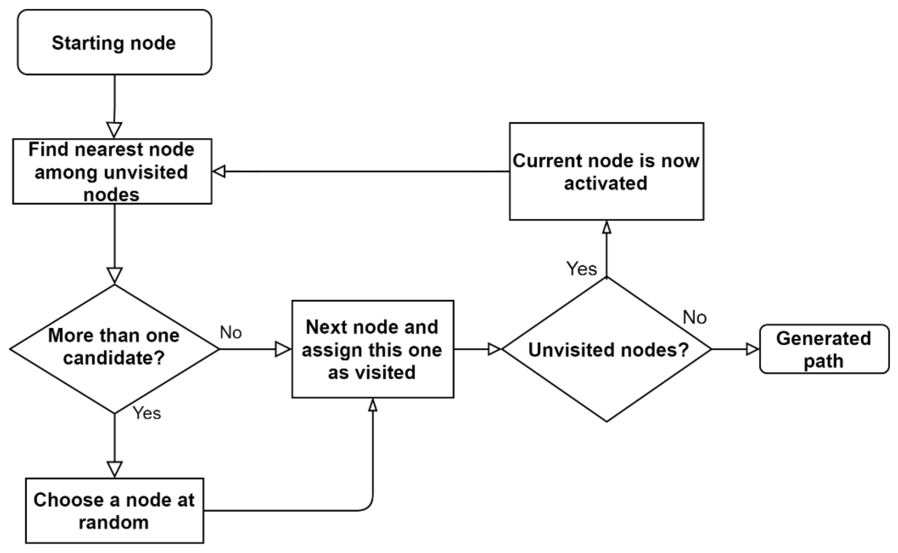
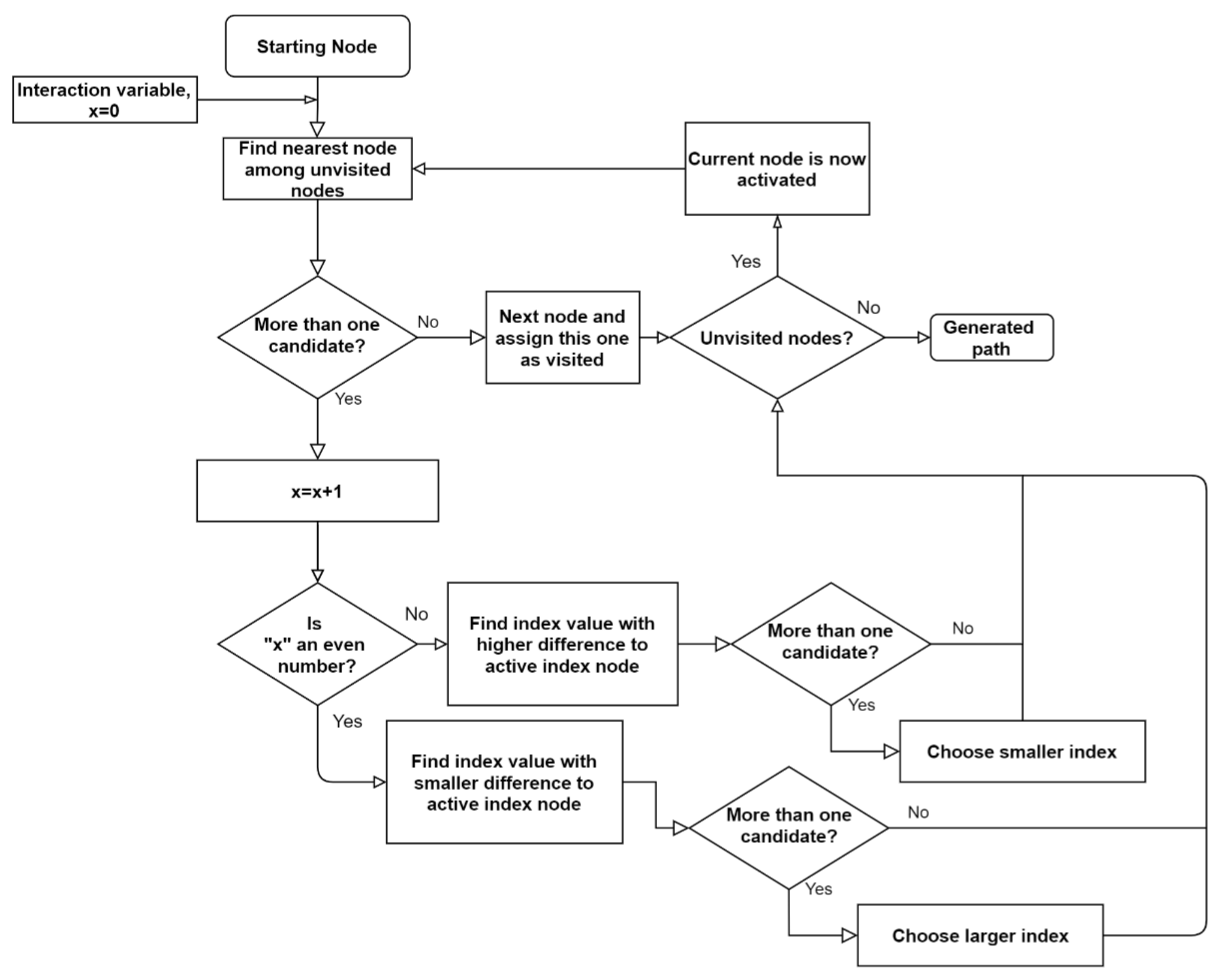
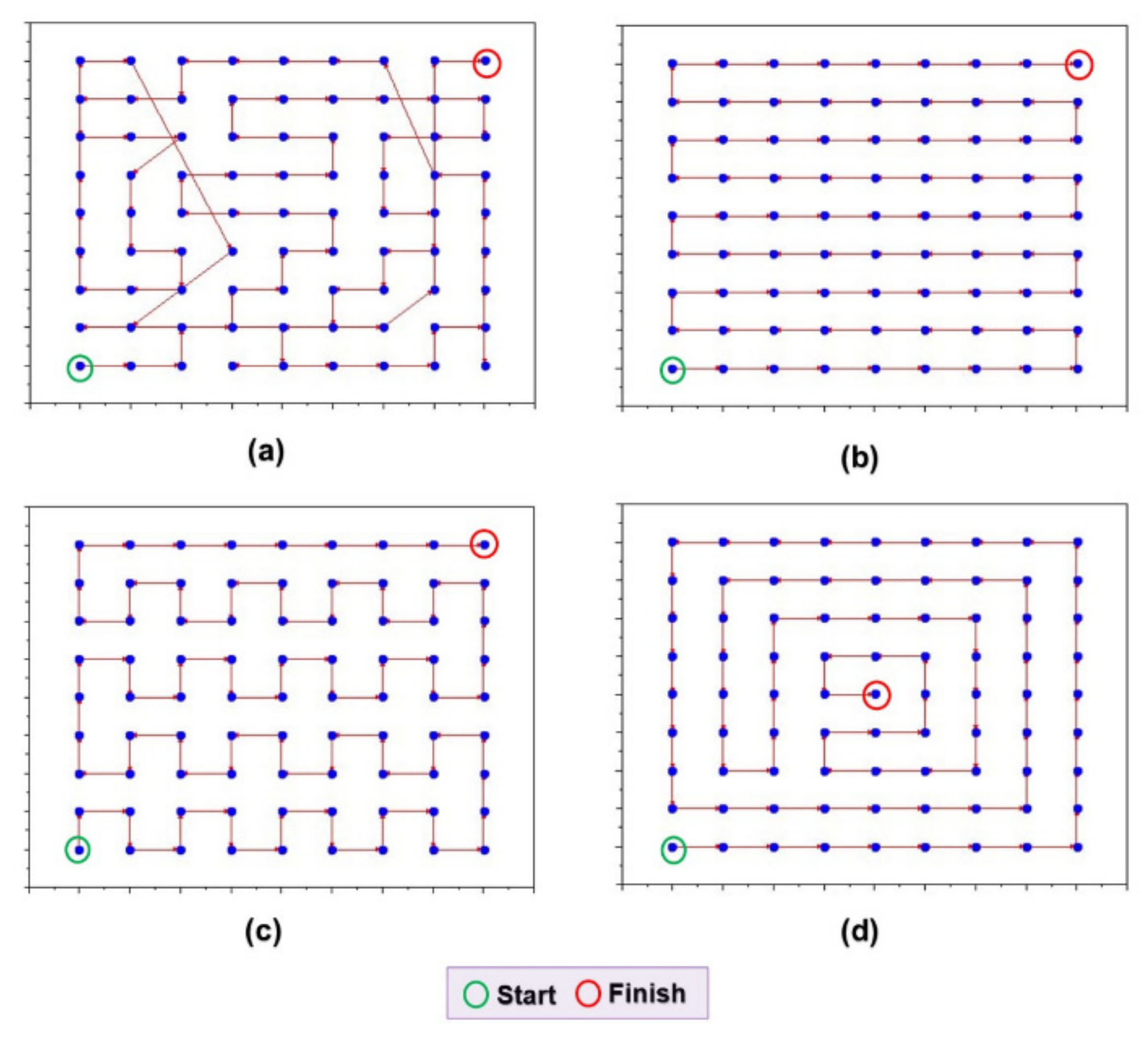
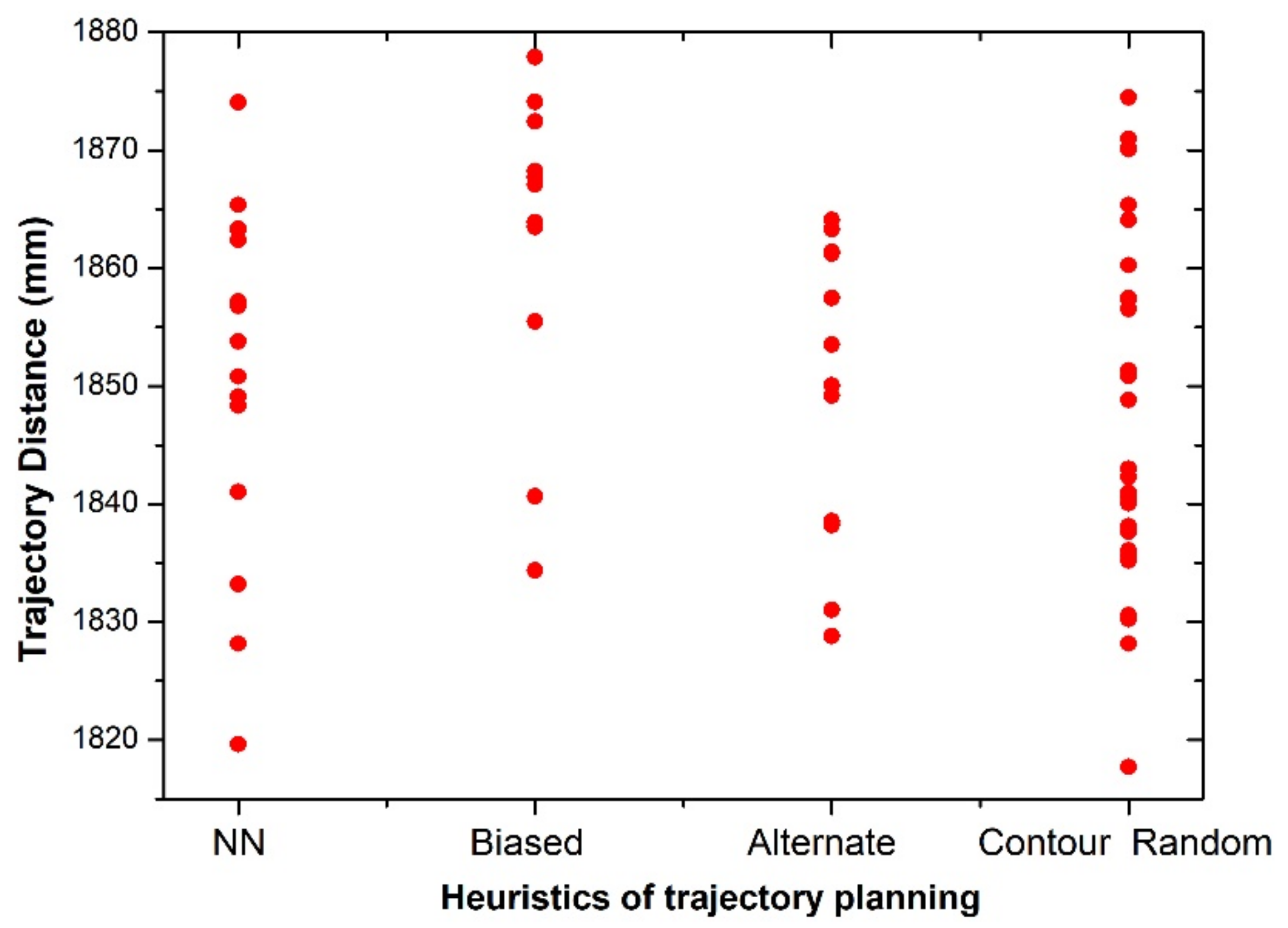
In Pixel trajectory deposition strategy, different heuristics of trajectory planning were used for sequential node connections (sometimes referred to as heuristics for simplification) following the TSP principle. The four heuristics employed in the current work are denominated nearest neighbor, biased, alternate and random contour, and they are described in the next subsections. Their goal was to force, with each of the heuristics, so as to have access by the algorithms to some of the strategies shown in Figure 2, yet under the concept of the Pixel strategy. For implementation of the heuristics in the Pixel strategy, a computer program was developed.

2.2.1. Nearest Neighbor Heuristic for Trajectory Planning

According to Aziz Ouaarab [13], the nearest neighbor heuristic is widely used for TSP solutions, and for this reason this heuristic was also applied in the Pixel strategy. Figure 8 shows a flowchart to schematize this heuristic for trajectory planning. The central idea is to select (as mentioned before, by raffling) an initial node to be visited (starting node) in any region of the discretized layer and from that to proceed to the shortest distance node (next node to be activated). The proximity criterion is based on the Euclidean distance, already presented in Equation (1). However, as the nodes generated on the surface of the layer are usually equidistant during the selection of the nearest node (Figure 9), more than one candidate with the same Euclidean distance is prone to appear. Among the candidate nodes, the algorithm will choose one at random and take it as the next activated node. The, till then, active node is reassigned as a visited node. In sequence, according to the proximity criterion, the cycle is repeated until there are no more unvisited nodes and a trajectory is generated by connecting one by one all discretized nodes in the layer.

2.2.2. Biased Heuristic for Trajectory Planning

Differently from the Nearest Neighbor heuristic, which was already known from literature, the biased heuristic was created for this work to force a zigzag deposition trajectory strategy. Figure 10 shows the flowchart of the biased heuristic, which is similar to the previous one, although presenting a difference in the decision-making when there is more than one equidistant candidate closer to active node, i.e., instead of random choice, there is a second scrutiny, which is based on the index value instead of the Euclidian distance. In this case, the node with the nearest index value is flagged and, if there is more than one unvisited candidate, the heuristic will pick up the one with succeeding index value. For example, in Figure 9 the next node to be activated after in would be in+1, despite the fact that there would be four equidistant nodes (in−1; in−m; in+1; in+m) and two preceding and succeeding index value nodes (in−1; in+1).

2.2.3. Alternate Heuristic for Trajectory Planning

The alternate heuristic flowchart is presented in Figure 11. Similar to the biased heuristic, the alternate heuristic was specifically created for the Pixel strategy, aiming at imposing torch oscillation during deposition, a technique commonly used in welding. This heuristic name comes from the decision is do welding alternately when there is more than one equidistant candidate to the next node. In this case, if the routine interaction takes an odd value, the node to be activated will be the node with the index value that presents a higher difference to the active index node. In the case of more than one candidate, the candidate with the smaller index value will be activated. Alternatively, in the case of even interactions, the node to be activated will be the node with the index value that presents the shortest difference to the active index node. In the case of more than one candidate, the one with the longest index value will be activated. Using Figure 9 again as an example, at first interaction, for which x = 0 (odd), the next node to be activated would be in−m, because it has greater index value difference from in and it is the one with the smaller index value between in−m and in+m. The subsequent node after in−m would be in−m+1.

2.2.4. Random Contour Heuristic for Trajectory Planning

The random contour heuristic is another heuristic created for the Pixel trajectory planning to pursue contour deposition trajectory strategy. According to its flowchart presented in Figure 12, when a draw happens between the closest candidates (equidistance criterion), decision-making is made in favor of the node that is closest to the polygon edges (internal and external). In the case that there is still a draw, the decision is made at random between the drawn nodes. To exemplify this latter case using Figure 9 again, the nodes in−m (vertically) and in−1 (horizontally) would be equidistant to in, but equivalent as nodes closest to the polygon edges, taking into account all directions. In this case, a choice at random would be made to define one of the two alternatives.

2.2.5. Examples of Trajectories Generated by the Four Heuristics

For a better visualization of the different heuristics of trajectory planning applied by the Pixel strategy, Figure 13 illustrates their application on a polygonal square-shaped surface. By way of example, all heuristics have taken node 1 as a starting node. Figure 13a illustrates the trajectory generated by nearest neighbor heuristic. The trajectory generated by the biased heuristic (Figure 13b), in turn, is very similar to the zigzag strategy, but modelled by dots rather than segments. In Figure 13c, where the alternate heuristic was tested by the algorithm, the trajectory is typically a square wave-shaped oscillation. Finally, in Figure 13d is shown how the random contour heuristic would present the trajectory, similar to the spiral contour strategy.
As seen, the objectives of each the heuristics were reached. Naturally, with a random choice of the starting node and recursively running the heuristic algorithms, different trajectory patterns could result. The total trajectory distances (DT), used for decision-making among the delivered options, are, and would be, certainly different. However, this issue is out of scope of the current work.

2.3. Trajectory Optimization

Trajectories in WAAM should preferably be continuous, or with minimal interruptions, to reduce manufacturing time and improve the surface homogeneity of the printed parts (the shorter the route, the better the objective function of the optimization). For this, the paths generated (node connections to define a trajectory) in the previous subsections must always connect neighboring nodes, yet never pass through nodes already “visited” or present path crossing (which will result in accumulation of material in these regions). In Figure 13a, for example, the nearest neighbor heuristic presented path crossings, which showed the need for improvement. In the other heuristics, although they did not present path crossings, the algorithms could deliver trajectories with path crossings as a function of other starting nodes and/or higher geometry complexity. Paths with no deposition (“empty” trajectories) to avoid path crossing, in turn, can be adopted, however, at the expense of arc stops and starts (regions predisposed to imperfections) and potentially increased manufacturing time. Therefore, penalties are inserted in the algorithm when path crossings (and other constraints) are identified (first optimization constraint factor).
To perform optimization for the objective function, Equation (2), and constraints in the Pixel strategy, a local search through the 2-opt algorithm, commonly used as heuristics of improvements for TSP [16], was initially applied. This improvement consisted of initially choosing two paths between the nodes of the generated trajectory and reversing their connections to verify if a reduction in path distance would occur. Figure 14a presents an example where path 1 initially chosen by one sequential node connection heuristic was represented by node A interconnected to node B and path 2 represented by node C interconnected to node D. When applying the 2-opt algorithm, the chosen paths were undone and uncrossed, that is, node A now generated a path connecting to node C, and node B generated a path interconnected to node D, as illustrated in Figure 14b. If there is a reduction in the Euclidean distance, the new solution is adopted, otherwise the swap is undone and another pair of neighboring nodes is chosen and the process is repeated over and over again. This operation is repeated until no further improvements occur with path crossings. With this, a great local solution is obtained.
Despite the good results obtained by the 2-opt heuristic, this technique is restricted to a maximum or minimum local only (such as entering a valley or climbing a peak of the search space). In order to allow exploration of other valleys/peaks in the space, the local search is boosted by previously using the metaheuristic greedy randomized adaptive search procedure (GRASP), which consists of a higher-level heuristic procedure designed to find a better solution to an optimization problem. GRASP basically consists of a multiboot iterative technique of global search from successively constructed randomized solutions and subsequent iterative improvements of the same. According to Sohrabi et al. [17], each iteration performs two perfectly defined phases. According to these authors, the first phase creates viable solutions to the problem, which promotes diversity, and the second phase consists of the optimization from the created solutions.
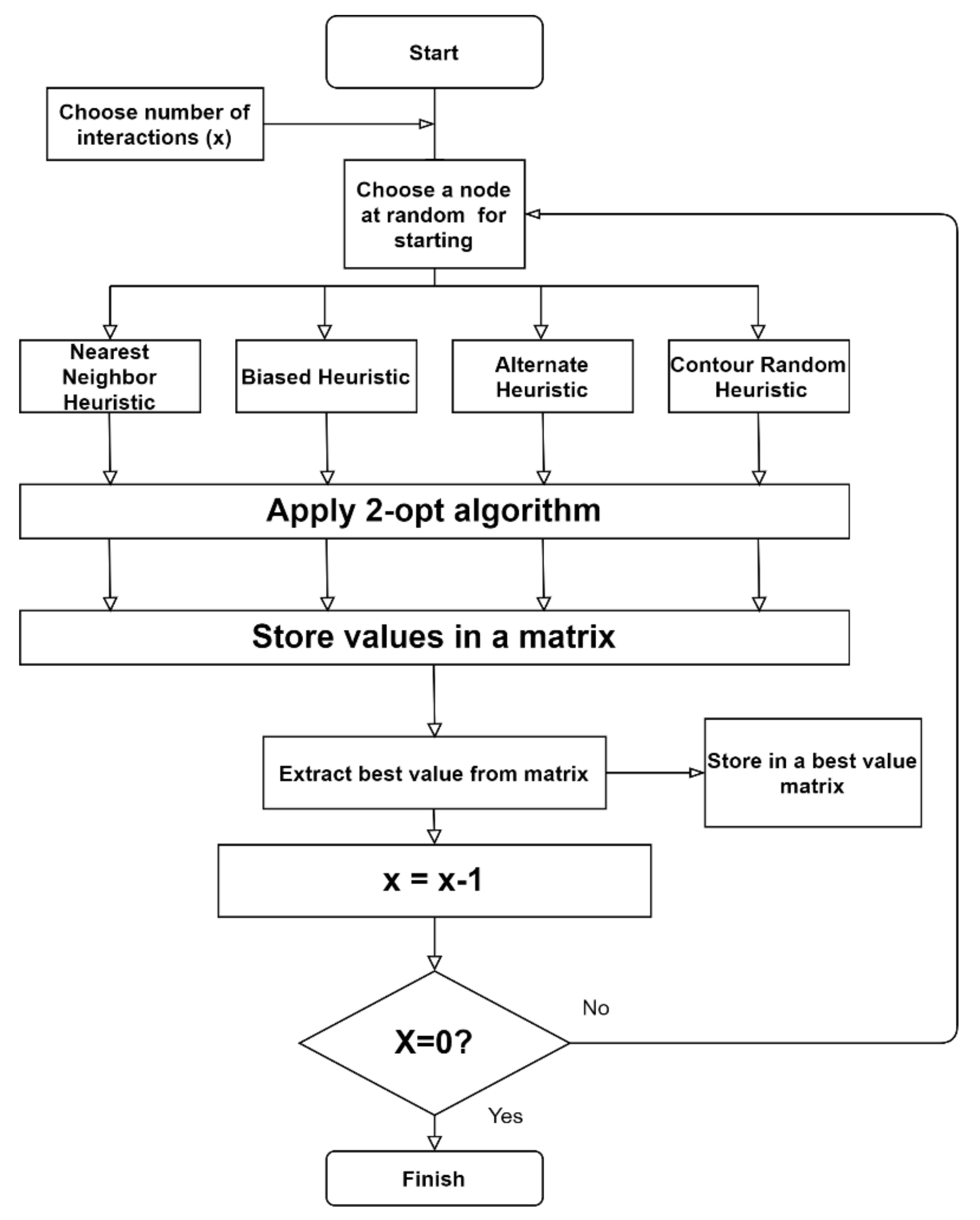
Figure 15 shows the GRASP flowchart adapted to the Pixel strategy for WAAM, which starts with the input of the number of interactions from the process analyst. After a random selection for picking up the starting node, the algorithm performs the trajectory planning using the four heuristics presented in the previous section, that is, the nearest neighbor heuristic, the biased heuristic, the alternate heuristic and the random contour heuristic. After that, each of them is optimized with the 2-opt algorithm, which will result in four values of local minima. The lowest value obtained (shortest route, unless defined other objective function) is stored in an array of best values. Then, a subsequent interaction is performed until the number of interactions is zeroed out. In this application of GRASP, the loop resumes from the random selection of a new starting node, which allows diversity in the initialization phase and a global exploration of the search space.
One outstanding point of this adaptation is that GRASP has an array of better values and related metrics as outputs. At first, the process analyst chooses the trajectory that will print the part, usually based on the shortest distance, already avoiding the path crossings and node visit duplication. To monitor the functionality of the Pixel strategy, the algorithm delivers a report that relates the trajectories of the best value matrix to its heuristics of trajectory planning. With this, it is possible to check if there is tendency of one or more heuristics of trajectory planning to always generate the shortest routes (a self-learning evaluation for the process analyst).
This strategy is useful for the process analyst to make decisions systematically, considering that the algorithm can be executed with all four heuristic of trajectory planning, or only with the selected ones. The latter option reduces the computational time to generate the trajectories. As another alternative to reduce computational time, the algorithm’s stop criterion is optionally added for when the first trajectory without path crossings is found, as it would already be a viable trajectory for WAAM.

3. Evaluation of the Pixel Path Planning Strategy

3.1. Computational Evaluation

A slice in the shape of a nonconvex polygon (Figure 16a) was chosen as the case study for the computational evaluation of the Pixel trajectory strategy approach. This geometry symbolized a more difficult condition for WAAM, yet not too complex to be analyzed and explained here. First, the piece was sliced (Figure 16b) with a given increment (in this case, 2.2 mm). Figure 16c displays the top view of one of the layers to be treated by the Pixel strategy. Starting with the discretization of the layer, an initial internal offset of a given distance (in this case, 4.5 mm) from the polygon edges was implemented (Figure 16d). The spacing between the dots was set (in this case, 6 mm), with the grid starting from the left-most and lower sides of the offset (Figure 16e), totaling 303 nodes generated on the surface. Finally, the adapted GRASP metaheuristic procedure (which encompasses the 2-opt local search algorithm) was used to generate optimized trajectories. Seventy-six interactions were used, equivalent to 25% of the total number of nodes (this percentage was arbitrarily chosen). As a result, a matrix of best values was fed with the 76 optimized trajectories. Figure 16f illustrates the obtained shortest trajectory, which was reached by the random contour heuristic.
Figure 17 presents the matrix of the best values in graphical form. Each point represented the best trajectory of an interaction. In the abscissa, the 4 heuristics of trajectory planning were indicated, so that one could see the number of shortest distances per interaction resultant from each heuristic, as well as the longest and shortest distances after all interactions. It can be seen that the random contour heuristic was the most efficient, with the highest number (28) of shortest distances after 76 interactions, against 24 of the nearest neighbor, 13 of alternate and 11 of biased. In the study case, the random contour heuristic was that which also produced the shortest trajectory among the whole array, with 1817.72 mm, followed closely by the nearest neighbor heuristic, with 1819.61 mm. On the other hand, the same random contour also produced the second longest trajectory among the shortest trajectory per interaction. This reinforces the casual character of the process. Therefore, it is important to understand that both other geometry and a different number of interactions (or even a new run of the GRASP algorithm), could deliver other results concerning the most efficient heuristic of trajectory planning.
However, although the random contour heuristic has the lowest trajectory value, the other heuristics also generated continuous trajectories that may be feasible for WAAM of this prismatic shape. Given the above, the matrix of better values provides other continuous trajectories, but it is up to the process analyst to choose the trajectory that will print the part. This human control of the results allows the specialist to opt for another trajectory, privileging other important requirements for the printed part (such as better mechanical strength, less distortion or better surface quality). Therefore, the experience of the process analyst is important for the success of the process. Notwithstanding, studies will be carried out in a near future to automate this decision-making through smart algorithms (multiobjective optimization and/or machine learning).

3.2. Experimental Evaluation

Two geometries (to be detailed later) were WAA Manufactured using the trajectory planning developed with the Pixel strategy. A CNC gantry dedicated to WAAM was used for the torch X-Y-Z movements. The deposition was carried out using Fronius CMT equipment (Fronius International GMBH, Wels, Austria) over a substrate made of a SAE 1020 steel plate, with dimensions of 300 × 180 × 12 mm3. The substrate was cooled with water (immersed), characterizing a passive thermal management. Further details of the experimental rig can be found in Silva et al. [18]. A 1.2-mm-diameter AWS ER70S-6 class wire was employed, with the arc shielded by a blend of Ar and CO2 (4%). The contact tip-to-work distance was set at 12 mm. The deposition and wire feed speeds were 32 cm/min and 4.1 m/min, respectively, leading to 2.8-mm-high and 4.1-mm-wide straight paths.
Therefore, the inputs to the program to perform the Pixel strategy were an offset distance of 2 mm (half-width of the deposited paths) and the distance between the nodes was fixed at 3.03 mm, considering the 73.8% of path overlapping of the bead width suggested by Ding et al. [19]. It is noteworthy that parameter optimization for printing was not adopted, because it would be out of the work scope, even though the authors recognize that proper parameterization is crucial to reach sound trajectories. These deposition parameters and path planning were used for both geometries.
Figure 18 presents the prismatic shape of the first geometry, the trajectory planned by using the Pixel strategy (utilizing 383 nodes, after 50 interactions with the four heuristics without any algorithm stop criterion, having the biased as heuristic of trajectory planning and totaling 1253 mm of trajectory per layer) and the top surface of the part after printing. This geometry (a nonconvex polygon) mimics the one used by Ding et al. [9], which is not easily printed by the traditional contour or zigzag strategies. Six layers were printed on the top of each other with the trajectory shown in Figure 18a, with a dwell time of 120 s between layers (one start and one stop per layer). The optimized trajectory followed basically a zigzag pattern at the first half of the layer area, but with self-adjustment of the infill pattern accordingly to the distances between beads and between the end of the track and the polygon edges. The zigzag took a slightly different pattern at the second half of layer area, all decided by the algorithm after the 50 heuristic interactions. This was also noted at the last track, where the adjustment was made with an oscillation-like trajectory. This changing behavior happens because the dimensions of the layers will not be always an integer multiple of the distance between beads.
Figure 19, in turn, presents the second geometry, based on a similar shape presented in Wang et al. [6]. This geometry is also a nonconvex polygon, yet even more complex than geometry 1, due to two inner holes. Most of the strategies presented in the introduction suggested that this geometry could not be performed by continuous printing. However, the continuous trajectory planned by using the Pixel strategy for geometry 2 was reached by utilizing 1072 nodes after 50 interactions with the four heuristics without algorithm stop criterion, having the random contour as heuristic of trajectory planning and totaling 3038.70 mm of travel per layer. Six layers were printed on top of each other with the trajectory shown in Figure 19a, with a dwell time of 120 s between layers (also just one start and stop per layer). The trajectory assumed a maze-like behavior, in which an infill pattern made the deposition to contour the circumference of the holes. It is noted that the trajectory first skirted the edges of the layer and then filled in the part, due to the fact that its origin was the random contour heuristic.
For both geometries, the Pixel strategy showed itself to be efficacious. It is noteworthy that the trajectory chosen within the matrix of best values was that with the shortest path. However, better results could have been obtained from other runs of the algorithm. This explains that the algorithm generates more than one viable trajectory for printing, in the same execution (within the array of best values) or in different executions. However, small geometric irregularities can be seen mainly at the edges and vertices of the geometries. These nonconformities, due to the molten pool format, can be removed by machining, which will leave the near net shape part with the designed nominal dimensions. It is important to mention that the quality of the parts printed by this strategy can be further improved. Analyses will be performed to verify the surface quality, porosity and potential mechanical strength improvement. In the case of nonconformity verification, restrictions in the optimization process and/or use of machine learning algorithms will be used to obtain a path that does not generate defects.
The parts shown in these case studies are relatively small (but complex and bulky). In this study, the maximum number of nodes was 1072, therefore it is also important to state that a hybrid approach between Pixel and polygonal division strategy can increase the trajectory efficiency in the case of larger parts. With this hybrid approach, computational time can be reduced because the layer to be printed would be divided into smaller polygons that would have reduced numbers of nodes, which make it easier to find an optimized trajectory. In layers with symmetrical geometries, the trajectory can be planned only in one part of the geometry and mirrored to the following part(s), with minor changes to the algorithm. In this case, the number of nodes used to generate the trajectory will be less than if it were generated for the entire part. As future work, this innovative strategy opens up a range of alternatives. Regarding the heuristic of trajectory planning, new approaches can be thought to ensure better results after the optimization phase. In relation to optimization (without changing the Pixel concept for layer discretization and the heuristics for trajectory planning), other methods can be used, such as genetic algorithm, particle swarm algorithm, simulated annealing algorithm and LinKernighan algorithm within heuristics and metaheuristics. In addition, multi-objective optimization can be applied to satisfy other goals beyond the shortest route. With this window of possibilities, the Pixel strategy can be extended to other AM techniques.

4. Conclusions

An innovative deposition trajectory strategy for WAAM applicable in bulky components with complex geometries, such as nonconvex polygonal layers, with or without obstacles, was proposed and evaluated. It was concluded that:
  • The discretization of the layers, through distribution of dots all over the layer surfaces, is a computationally feasible method to cover the whole layer outline. The approach of coincident dot elimination prevented material accumulation. Continuous trajectories are reachable by using the travelling salesman problem (TSP) approach, since an intrinsic restriction of the approach is the reduction of arc extinction and restrikes and the impossibility of replicated node positions. The reach of TSP was enlarged by the Pixel strategy by obliging the algorithm to apply penalties to avoid other restraints, such as crossing paths. The created heuristic forced node connections to mimic the classical and successful strategies for trajectory planning. The trajectory optimization carried out by 2-Opt (local search) reduced the trajectory distances and the greedy randomized adaptive search (GRASP) metaheuristic allowed the global search for the optimized trajectory in acceptable computer time and resources;
  • The computational evaluation demonstrated that the option of having the four heuristics for node connections was the right decision, because the best heuristic was dependent on the geometry of the parts and all of them could be tested in the optimized outcome. Therefore, Pixel strategy is more flexible than classical approaches in this concern;
  • The experimental build WAA manufactured with GMAW and plain carbon steel showed that the Pixel strategy allowed continuous deposition and construction of difficult shapes, as in the case of polygonal nonconvex geometry with holes, with surfaces compatible to those typical for WAAM.

Author Contributions

R.P.F.: conceptualization, development, computational and experimental implementation, original draft preparation and editing; A.S.: supervision, contextualization, writing revision. All authors have read and agreed to the published version of the manuscript.

Funding

This work was partially funded by the National Council for Scientific and Technological Development—CNPq (grant number 302863/2016-8).

Institutional Review Board Statement

Not applicable.

Informed Consent Statement

Not applicable.

Data Availability Statement

This study did not report any data.

Acknowledgments

The authors would like to thank the Center for Research and Development of Welding Processes of the Federal University of Uberlândia (Laprosolda-UFU), Brazil, for the laboratory infrastructure and technical support. Special thanks to José Francisco de Castro Júnior and Henrique Nardon Ferraresi for technical support in the experiments.

Conflicts of Interest

The authors declare no conflict of interest.

References

  1. Rodrigues, T.A.; Duarte, V.; Miranda, R.M.; Santos, T.G.; Oliveira, J.P. Current status and perspectives on wire and arc additive manufacturing (WAAM). Materials 2019, 12, 1121. [Google Scholar] [CrossRef] [PubMed] [Green Version]
  2. DebRoy, T.; Wei, H.L.; Zuback, J.S.; Mukherjee, T.; Elmer, J.W.; Milewski, J.O.; Beese, A.M.; Wilson-Heid, A.; De, A.; Zhang, W. Additive manufacturing of metallic components -Process, structure and properties. Prog. Mater. Sci. 2018, 92, 112–224. [Google Scholar] [CrossRef]
  3. Gerdjikov, S.; Wolff, A. Decomposing a simple polygon into pseudo-triangles and convex polygons. Comput. Geom. 2008, 41, 21–30. [Google Scholar] [CrossRef] [Green Version]
  4. Liu, H.H.; Zhao, T.; Li, L.Y.; Liu, W.J.; Wang, T.Q.; Yue, J.F. A path planning and sharp corner correction strategy for wire and arc additive manufacturing of solid components with polygonal cross-sections. Int. J. Adv. Manuf. Technol. 2020, 106, 4879–4889. [Google Scholar] [CrossRef]
  5. Hu, Z.; Qin, X.; Shao, T.; Liu, H. Understanding and overcoming of abnormity at start and end of the weld bead in additive manufacturing with GMAW. Int. J. Adv. Manuf. Technol. 2018, 95, 2357–2368. [Google Scholar] [CrossRef]
  6. Wang, X.; Wang, A.; Li, Y. A sequential path-planning methodology for wire and arc additive manufacturing based on a water-pouring rule. Int. J. Adv. Manuf. Technol. 2019, 103, 3813–3830. [Google Scholar] [CrossRef]
  7. Dwivedi, R.; Kovacevic, R. Automated torch path planning using polygon subdivision for solid freeform fabrication based on welding. J. Manuf. Syst. 2004, 23, 278–291. [Google Scholar] [CrossRef]
  8. Ding, D.; Pan, Z.; Cuiuri, D.; Li, H. A practical path planning methodology for wire and arc additive manufacturing of thin-walled structures. Robot. Comput. Integr. Manuf. 2015, 34, 8–19. [Google Scholar] [CrossRef] [Green Version]
  9. Ding, D.; Pan, Z.; Cuiuri, D.; Li, H.; Larkin, N. Adaptive path planning for wire-feed additive manufacturing using medial axis transformation. J. Clean. Prod. 2016, 133, 942–952. [Google Scholar] [CrossRef]
  10. Ding, D.; Pan, Z.; Cuiuri, D.; Li, H. A tool-path generation strategy for wire and arc additive manufacturing. Int. J. Adv. Manuf. Technol. 2014, 73, 173–183. [Google Scholar] [CrossRef] [Green Version]
  11. Xiong, Y.; Park, S.; Padmanathan, S.; Dharmawan, A.G.; Foong, S.; Rosen, D.W.; Soh, G.S. Process planning for adaptive contour parallel toolpath in additive manufacturing with variable bead width. Int. J. Adv. Manuf. Technol. 2019, 105, 4159–4170. [Google Scholar] [CrossRef]
  12. Yang, X.S. Nature-Inspired Metaheuristic Algorithms, 2nd ed.; Luniver Press: Cambridge, UK, 2008. [Google Scholar]
  13. Ouaarab, A. Review of tour generation for solving traveling salesman problems. In Nature-Inspired Computation in Navigation and Routing Problems; Yang, X.-S., Zhao, Y.-X., Eds.; Springer Tracts in Nature-Inspired Computing; Springer: Singapore, 2020; pp. 85–102. [Google Scholar] [CrossRef]
  14. Zia, M.; Cakir, Z.; Seker, D.Z. Spatial transformation of equality-generalized travelling salesman problem to travelling salesman problem. ISPRS Int. J. Geo Inf. 2018, 7, 115. [Google Scholar] [CrossRef] [Green Version]
  15. Wasser, T.; Jayal, A.D.; Pistor, C. Implementation and evaluation of novel build styles in fused deposition modeling (FDM). Strain 1999, 5, 95–102. [Google Scholar]
  16. Lee, M.-T.; Chen, B.-Y.; Lai, Y.-C. A Hybrid Tabu Search and 2-opt path programming for mission route planning of multiple robots under range limitations. Electronics 2020, 9, 534. [Google Scholar] [CrossRef] [Green Version]
  17. Sohrabi, S.; Ziarati, K.; Keshtkaran, M.A. Greedy randomized adaptive search procedure for the orienteering problem with hotel selection. Eur. J. Oper. Res. 2020, 283, 426–440. [Google Scholar] [CrossRef]
  18. Da Silva, L.J.; Souza, D.M.; de Araújo, D.B.; Reis, R.P.; Scotti, A. Concept and validation of an active cooling technique to mitigate heat accumulation in WAAM. Int. J. Adv. Manuf. Technol. 2020, 107, 2513–2523. [Google Scholar] [CrossRef]
  19. Ding, D.; Pan, Z.; Cuiuri, D.; Li, H. A multi-bead overlapping model for robotic wire and arc additive manufacturing (WAAM). Robot. Comput. Integr. Manuf. 2015, 31, 101–110. [Google Scholar] [CrossRef] [Green Version]
Figure 1. Illustrations of the concept of (a) convex and (b) nonconvex polygons.
Metals 11 00498 g001
Figure 2. Examples of strategies for trajectory planning in WAAM: (a) raster; (b) zigzag; (c) continuous (adapted from Dwivedi and Kovacevic [7]); (d) continuous with the spiral contour; (e) water-pouring rule (adapted from Wang et al. [6]); (f) parallel contour; (g) spiral contour; (h) MAT, after medial axis transformation (adapted from Ding et al. [8]); (i) adaptive MAT (adapted from Ding et al. [9]); (j) polygonal division into simpler polygons (after Dwivedi and Kovacevic [7]); (k) convex polygonal division (adapted from Ding et al. [10]) and (l) convex polygonal division with sharp corner correction (adapted from Liu et al. [4]).
Metals 11 00498 g002
Figure 3. A basic process chain for WAAM, highlighting the workflow of the Pixel strategy for trajectory planning (within the dashed lines).
Metals 11 00498 g003
Figure 4. Discretization of a layer surface according to the Pixel strategy: (a) original polygonal layer contour; (b) insert of the inscribed offset contour and respective generation of red dots; (c) generation of blue dots; and (d) generation of green dots.
Metals 11 00498 g004
Figure 5. Coincident and almost coincident dots during the discretization stage of a layer.
Metals 11 00498 g005
Figure 6. Indexing of nodes by ordering intersected dots distributed on a layer surface.
Metals 11 00498 g006
Figure 7. Diagram using the travelling salesman problem (TSP) to define a hypothetical trajectory as done in the Pixel strategy for WAAM.
Metals 11 00498 g007
Figure 8. Nearest neighbor heuristic for trajectory planning flowchart.
Metals 11 00498 g008
Figure 9. Index representation of a target node and its nearest neighbors.
Metals 11 00498 g009
Figure 10. Biased heuristic flowchart for trajectory planning.
Metals 11 00498 g010
Figure 11. Alternate heuristic flowchart for trajectory planning.
Metals 11 00498 g011
Figure 12. Random contour heuristic flowchart for trajectory planning.
Metals 11 00498 g012
Figure 13. Trajectories generated by the heuristic with a single interaction and using the same starting node: (a) nearest neighbor; (b) biased; (c) alternate; (d) random contour.
Metals 11 00498 g013
Figure 14. The 2-opt method for local search optimization in the Pixel trajectory strategy: (a) initial trajectory; and (b) trajectory optimized by uncrossing two paths.
Metals 11 00498 g014
Figure 15. GRASP metaheuristic flowchart used for the global search in the Pixel trajectory planning strategy.
Metals 11 00498 g015
Figure 16. Sequencing of the Pixel strategy used for trajectory planning of a case study (a nonconvex prismatic shape): (a) 3D CAD model (exportable as. stl format); (b) sliced model; (c) top view of polygonal layer (slice); (d) offset lines (4.5 mm edges) inscribed in polygonal layer; (e) nodes generated inside polygonal layer; and (f) shortest trajectory generated after 76 interactions.
Metals 11 00498 g016
Figure 17. Distances of result trajectories after each of the 76 GRASP interactions, as a function of the heuristics of trajectory planning.
Metals 11 00498 g017
Figure 18. Top view cross-section of a nonconvex polygon used as the first geometry printed using trajectory elaborated with Pixel strategy: (a) trajectory generated by Pixel strategy; and (b) 6-layer-high printed part.
Metals 11 00498 g018
Figure 19. Part with cross-section of nonconvex polygon and holes: (a) trajectory generated by Pixel strategy; and (b) printed part by Pixel strategy.
Metals 11 00498 g019
Publisher’s Note: MDPI stays neutral with regard to jurisdictional claims in published maps and institutional affiliations.

