Author Contributions
Conceptualization, S.K. and M.O.; methodology, S.D.V.K.; software, S.K.; validation, S.D.V.K. and S.K.; formal analysis, S.D.V.K. and S.K.; investigation, S.D.V.K.; resources, S.K.; data curation, S.D.V.K. and S.K.; writing—original draft preparation, S.D.V.K.; writing—review and editing, S.K. and M.O.; visualization, S.K. and M.O.; supervision, S.K.; project administration, S.K.; funding acquisition, S.K. All authors have read and agreed to the published version of the manuscript.
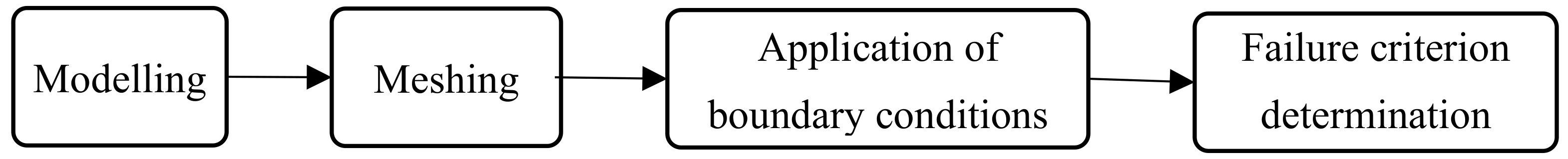
Figure 1.
Flow of the development of the FEM.
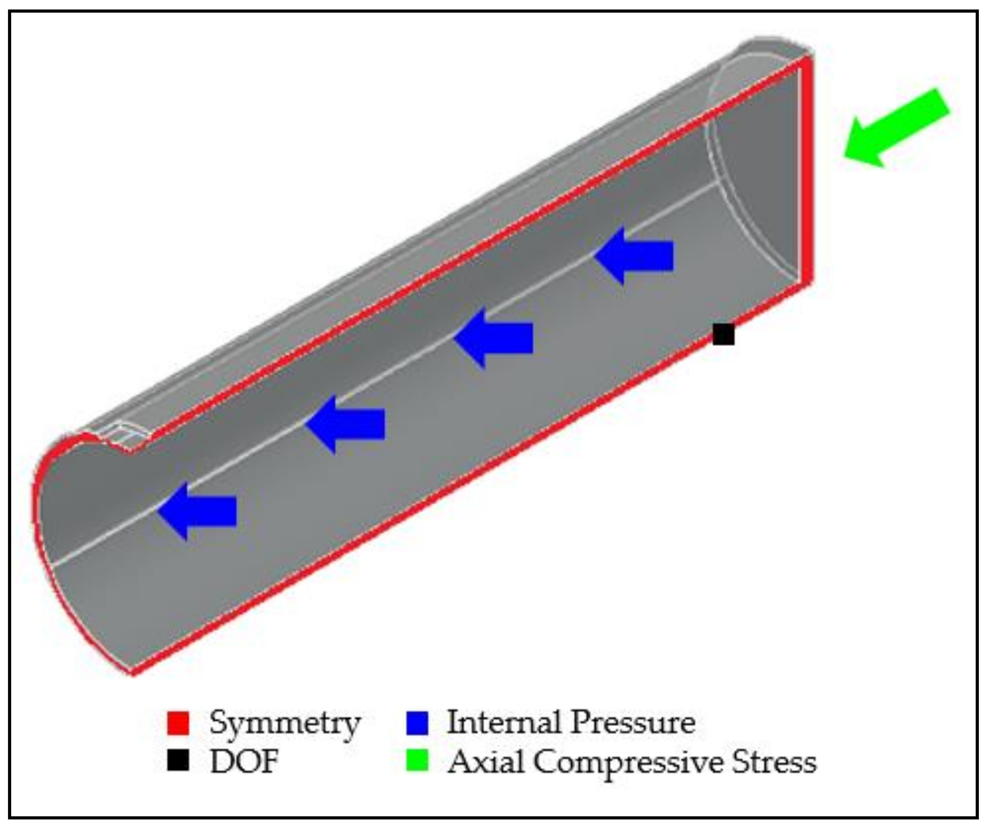
Figure 2.
An annotated quarter pipe model used for FEA.
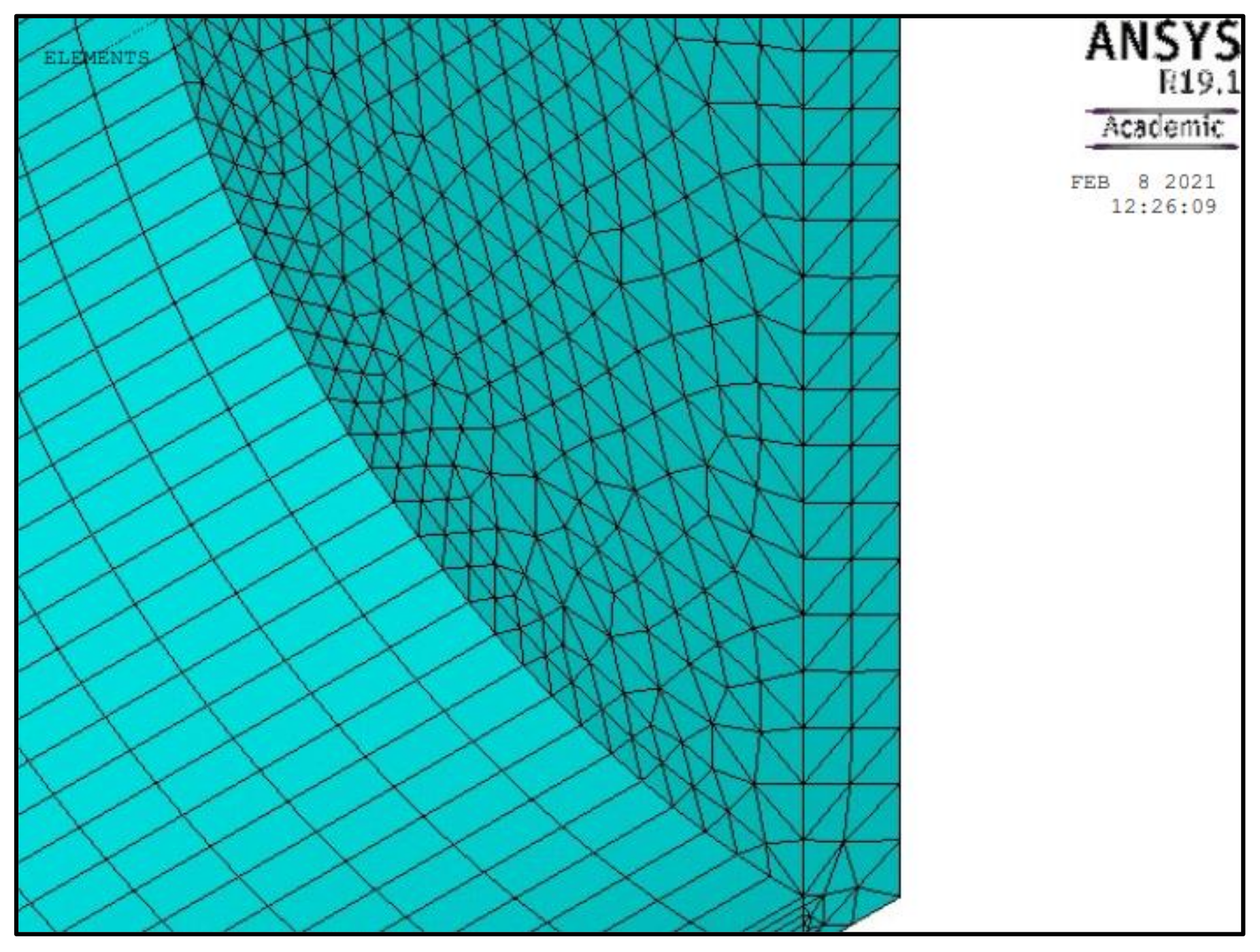
Figure 3.
Hexahedral SOLID185 elements used to mesh the pipe body and defect region.
Figure 4.
Tetrahedral SOLID186 elements used to mesh the endplate.
Figure 5.
Application of symmetrical boundary conditions, internal pressure, compressive stress, and degree of freedom (DOF) constraint for quarter pipe models.
Figure 6.
Red contour depicting the region of failure of the pipe.
Figure 7.
Flow of the development of the ANN.
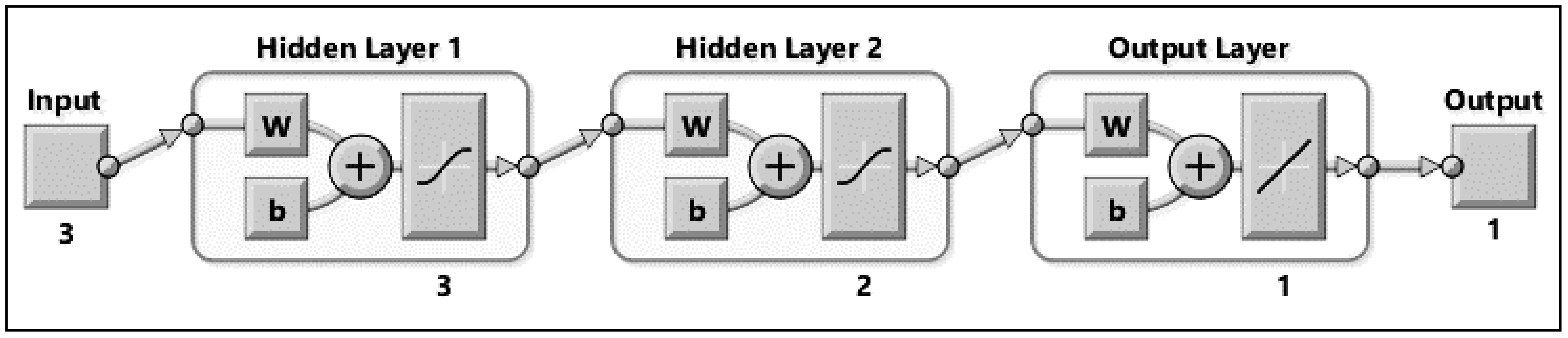
Figure 8.
Overview of the Artificial Neural Network (ANN) model.
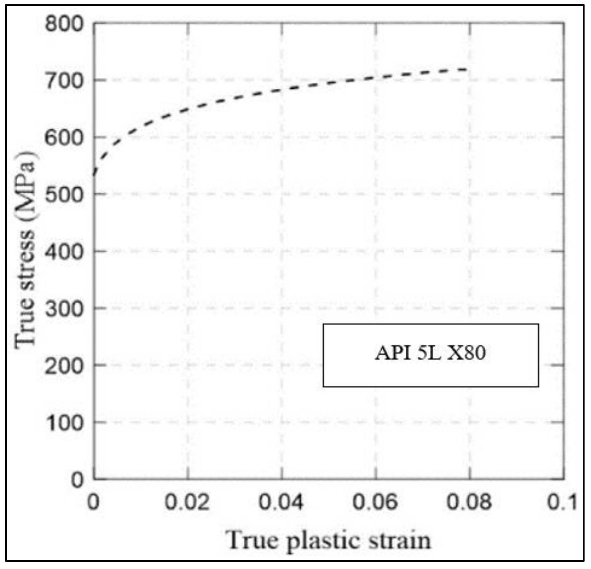
Figure 9.
True stress-strain curve for API 5L X80 steel, data from [
19].
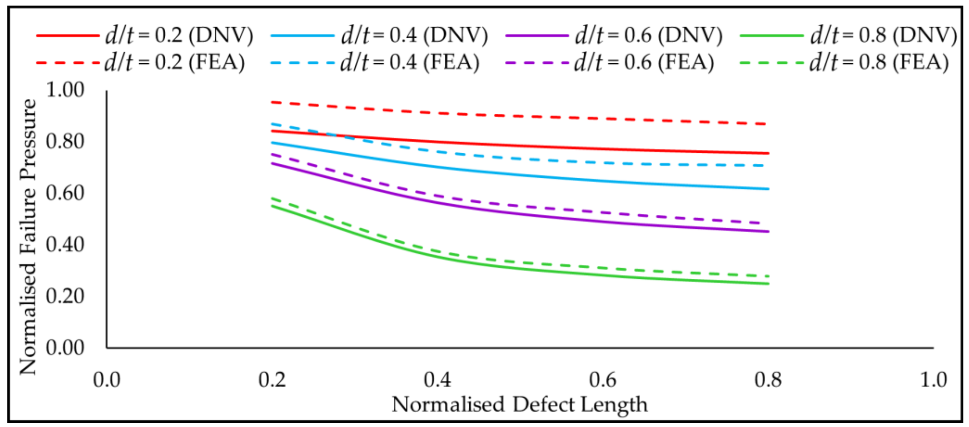
Figure 10.
Normalized failure pressure predictions of FEA and DNV for API 5L X80 pipe subjected to internal pressure only.
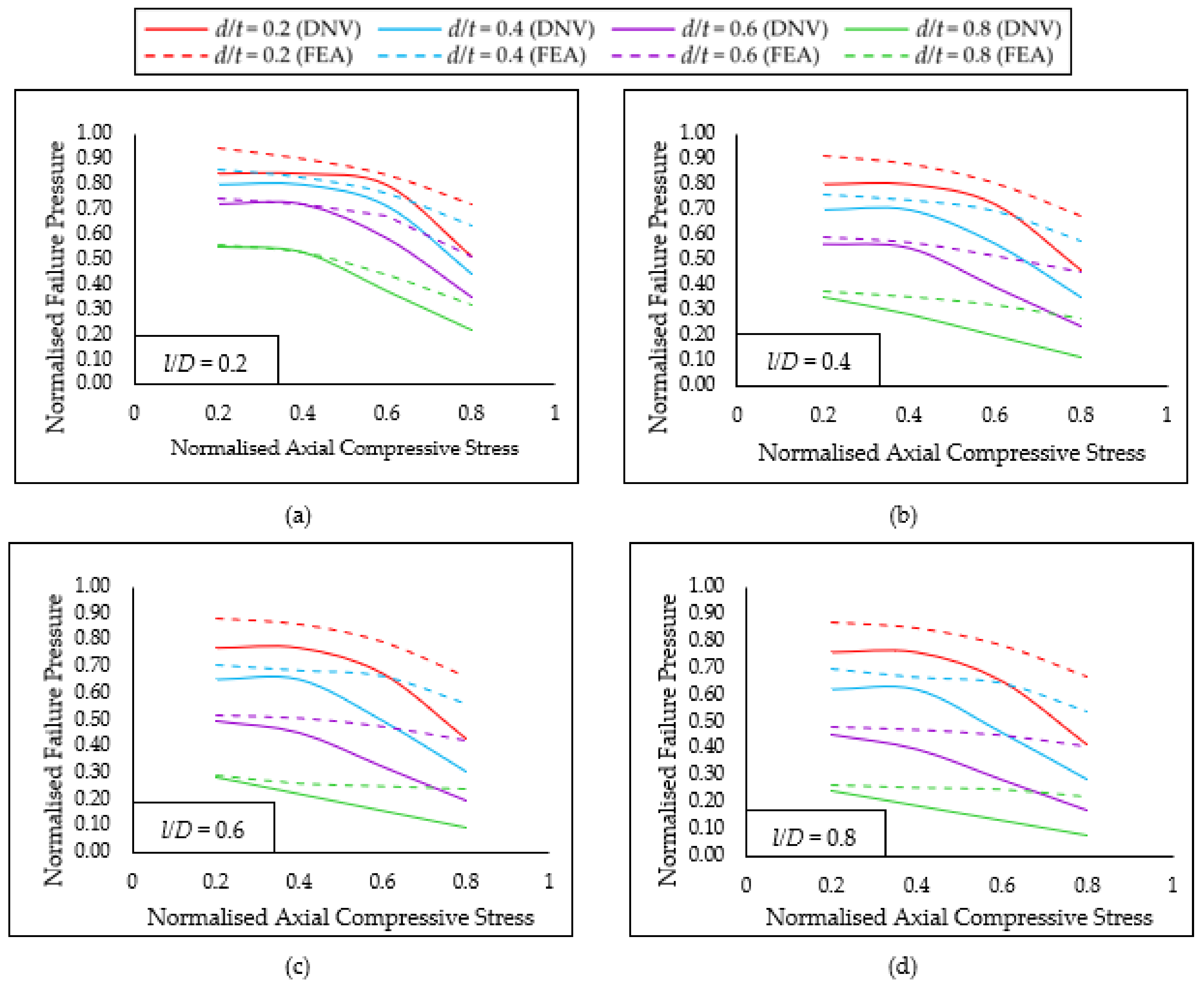
Figure 11.
(a) Normalized failure pressure predictions of API 5L X80 pipe using FEA and DNV subjected to internal pressure and axial compressive stress for a normalised defect length of (a) 0.2; (b) 0.4; (c) 0.6; and (d) 0.8.
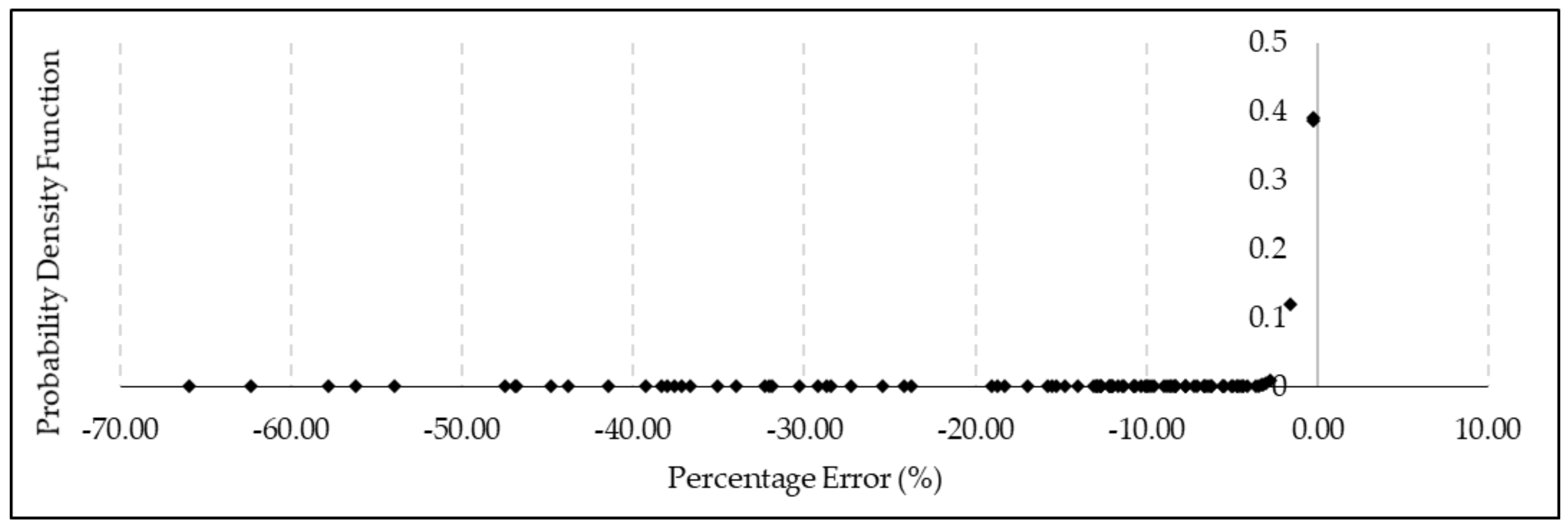
Figure 12.
Probability density function of normalized failure pressure predictions using DNV method when compared to FEM for API 5L X80 pipe subjected to internal pressure and axial compressive stress.
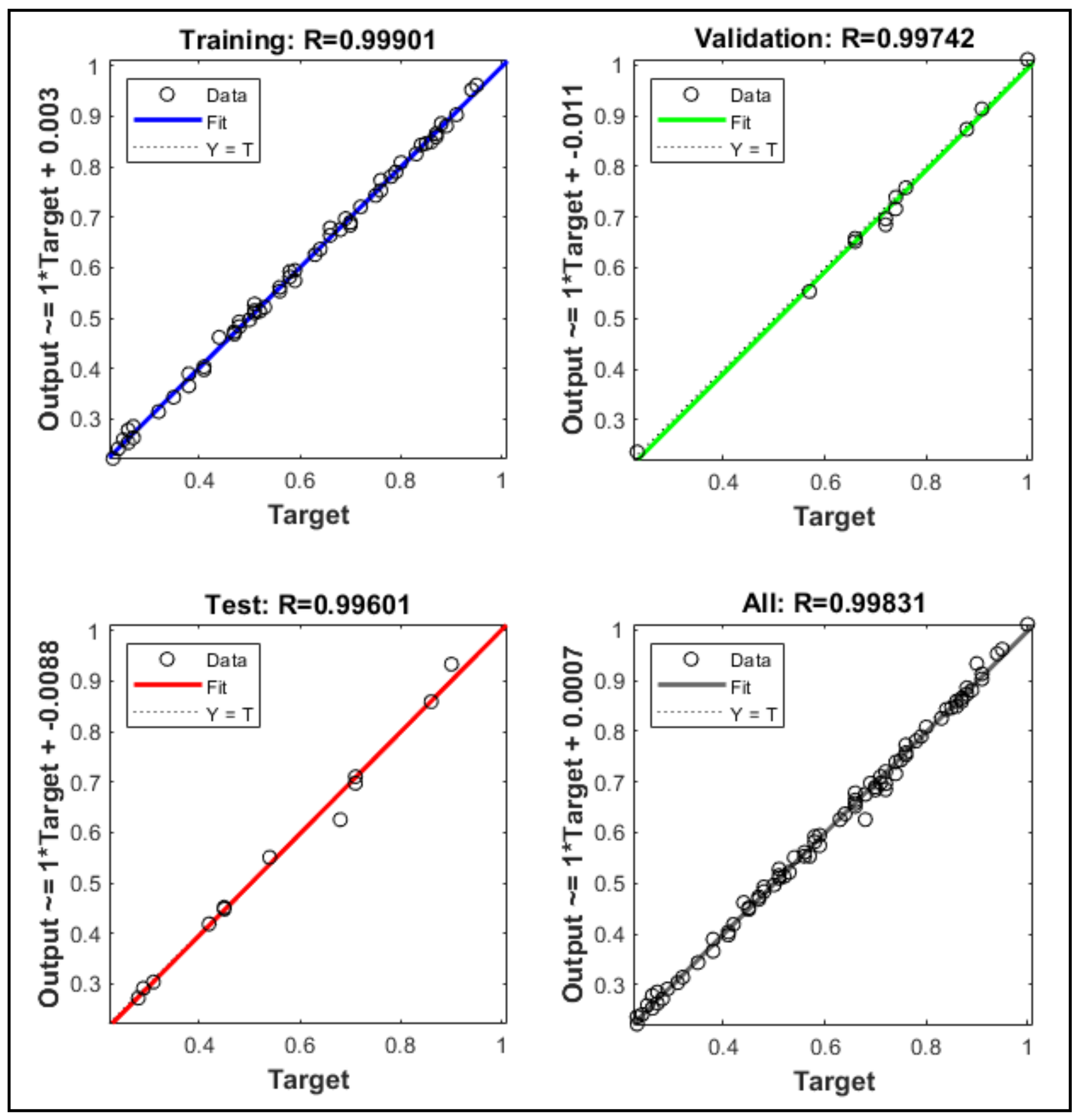
Figure 13.
Regression plots of Model 5.
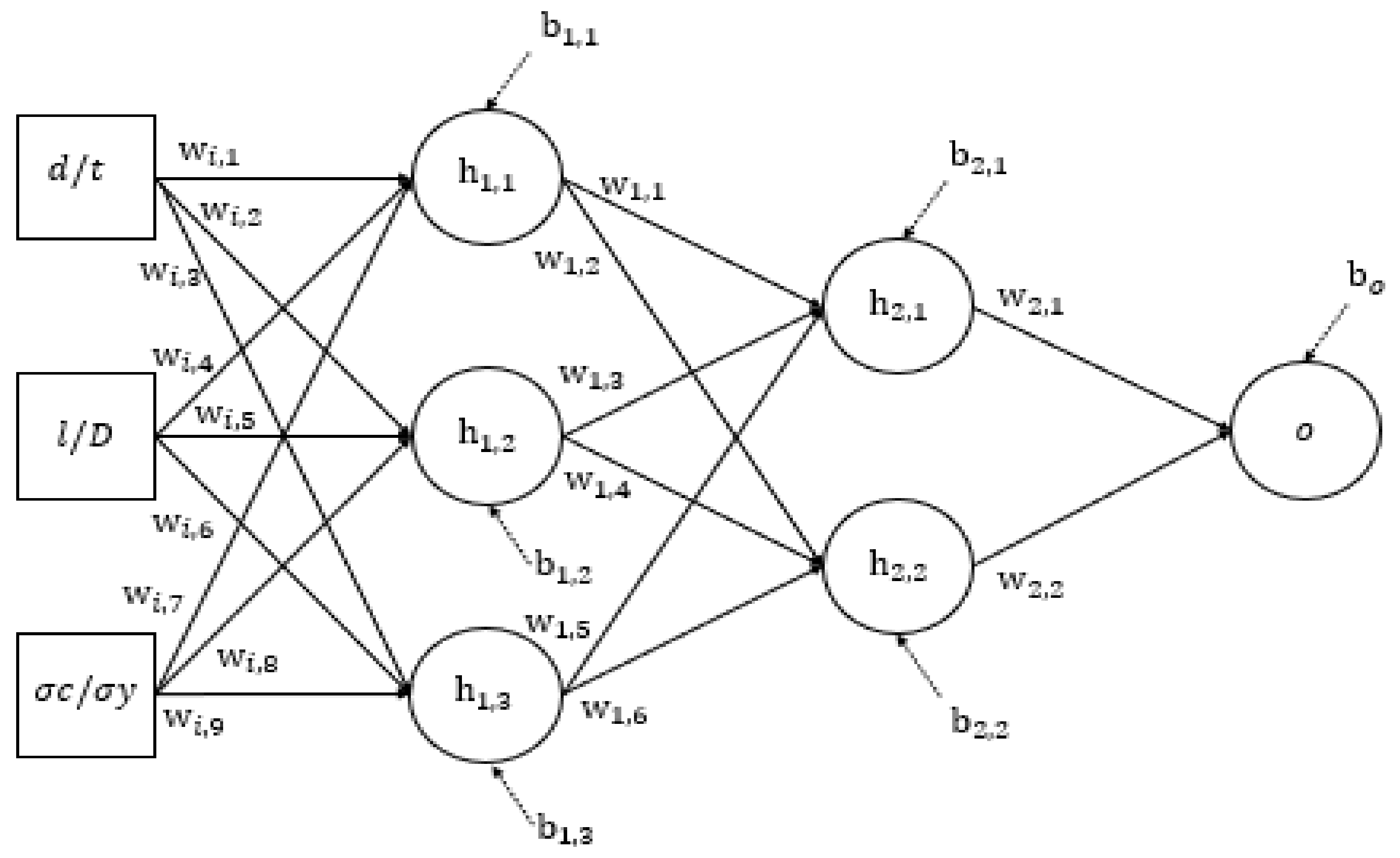
Figure 14.
Architecture of the ANN model.
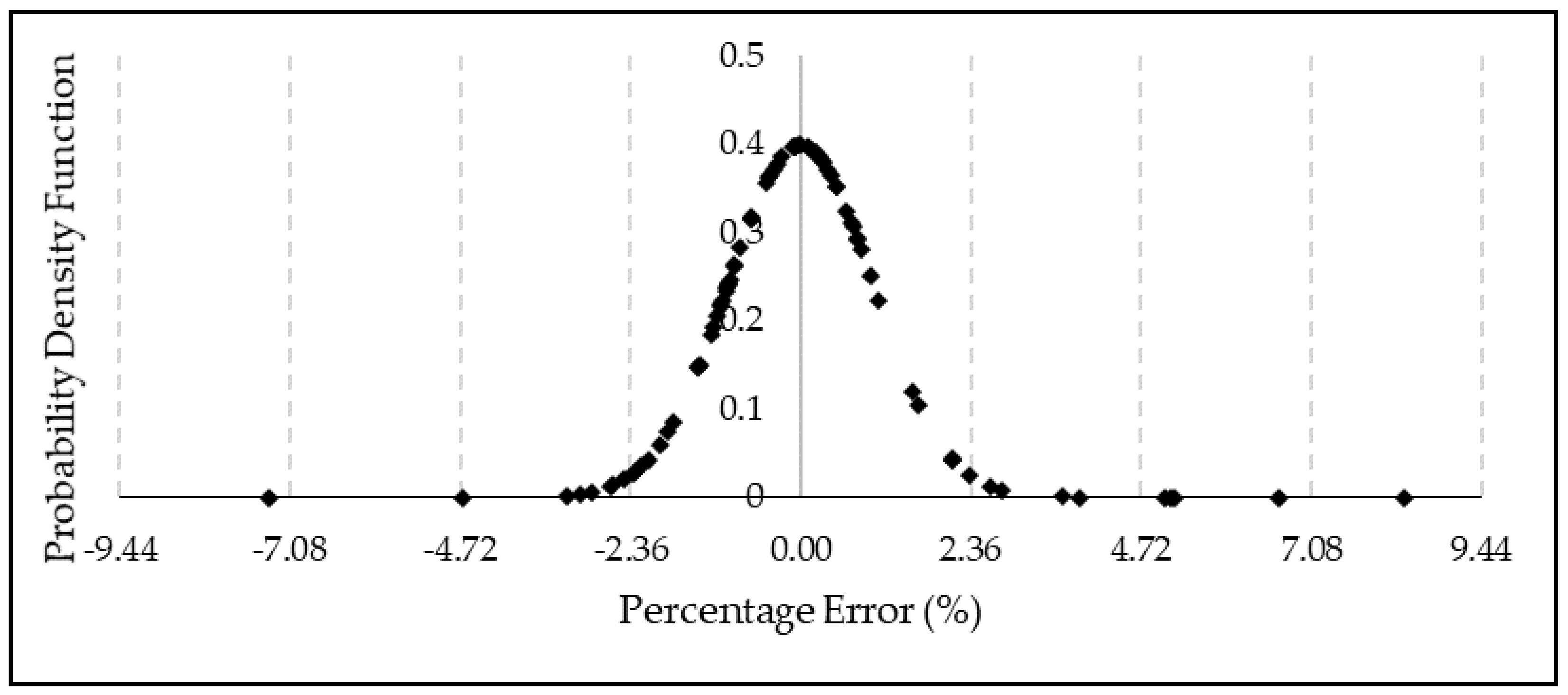
Figure 15.
Probability distribution of the percentage error obtained using the newly developed failure pressure prediction method and FEM based on the parameters of the ANN training data.
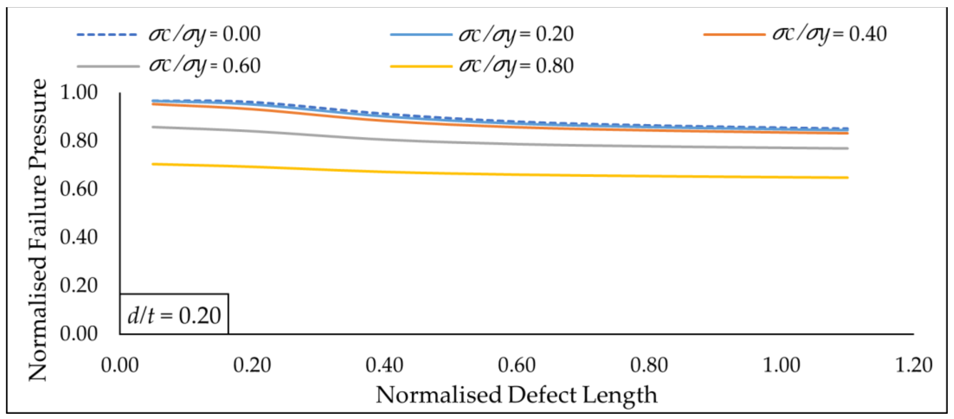
Figure 16.
Normalized failure pressure predictions of the new assessment method against various normalized defect length for multiple axial compressive stress at a constant normalized defect depth of 0.20.
Figure 17.
Normalized failure pressure predictions of the new assessment method against various normalized defect length for multiple axial compressive stress at a constant normalized defect depth of 0.80.
Figure 18.
Normalized failure pressure predictions of the new assessment method against various normalized defect length for multiple normalised defect depths at constant normalized axial compressive stress of 0.40.
Figure 19.
Normalized failure pressure predictions of the new assessment method against various normalized defect depth for multiple axial compressive stress at constant normalized defect length of 0.60.
Figure 20.
Normalized failure pressure predictions of the new assessment method against various normalized defect depth for multiple normalised defect lengths at a constant normalized axial compressive stress of 0.40.
Figure 21.
Normalized failure pressure predictions of the new assessment method against various normalized axial compressive stress for multiple normalised defect depths at a constant normalized defect length of 0.60.
Table 1.
Comparison of pipe failure pressure assessment methods.
| Method | Fundamental Equation | Governing Assumption | Material Restriction |
|---|
| ASME B31G | NG-18 | Tensile property of a pipe determines the mechanism that causes pipe failure. | Low toughness |
| Modified B31G | NG-18 | Low toughness |
| SHELL 92 | NG-18 | - |
| A Modified Criterion for Evaluating the Remaining Strength of Corroded Pipe (RSTRENG) | NG-18 | - |
| DNV RP-F101 | NG-18 | Pipe failure due to plastic collapse (plastic flow), where the ultimate tensile strength is the flow stress. | Moderate toughness |
| Pipe Corrosion Criterion (PCORRC) | Numerical studies | Moderate to high toughness |
Table 2.
Geometric parameters for finite element analysis (FEA) parametric study.
| Input Parameters | Value (s) |
|---|
| Outer diameter of pipe, (mm) | 300 |
| Wall thickness, (mm) | 10 |
| Straight pipe length, (mm) | 2000 |
| Defect width, (mm) | 100 |
| Normalized defect length, | 0.0, 0.2, 0.4, 0.6, 0.8 |
| Normalized defect depth, | 0.0, 0.2, 0.4, 0.6, 0.8 |
| Normalized axial compressive stress, σc/σy | 0.0, 0.2, 0.4, 0.6, 0.8 |
Table 3.
DNV corrosion assessment factors and assumptions.
| Factor | Value | Assumptions |
|---|
| Model prediction partial safety factor, | 1.00 | Perfect pipe inspection method. |
| Corrosion depth partial safety factor, | 1.00 | Exact corrosion defect depth. |
| Fractile value, | 0.00 | Low tolerance and high confidence level corrosion inspection method. |
| Usage factor, | 1.00 | Pristine pipe. |
| Relative depth accuracy, acc_rel | 0.00 | High corrosion depth inspection accuracy with zero tolerance. |
| Confidence level, conf | 0.99 | 99% confidence level on corrosion defect dimensions. |
Table 4.
Summary of FEA failure pressure validation against full-scale burst tests for pipes subjected to internal pressure only, and internal pressure and axial compressive stress, data from [
30,
31,
32].
| Author(s), Year | Bjornoy & Sigurdsson, 2000 | B. Ma et al., 2013 | Benjamin et al., 2005 |
|---|
| Grade | X52 | X52 | X52 | X65 | X80 |
| Specimen | Test 1 | Test 5 | Test 6 | Test 61 | IDTS 2 |
| (mm) | 5.15 | 3.09 | 3.09 | 4.40 | 5.39 |
| (mm) | 243 | 162 | 162 | 200 | 39.6 |
| (mm) | 154.5 | 30.9 | 30.9 | 50.0 | 31.9 |
| σl (MPa) | 0.0 | 48.0 | 84.0 | 0.0 | 0.0 |
| Burst Pressure (MPa) | 23.20 | 28.60 | 28.70 | 24.11 | 22.68 |
| FEA failure pressure (MPa) | 22.95 | 28.35 | 27.00 | 23.25 | 22.40 |
| Percentage Difference (%) | 1.08 | 0.87 | 5.92 | 3.57 | 1.23 |
Table 5.
ANN training data.
| | | | | | | | | | | |
|---|
| 0.0 | 0.0 | 0.0 | 1.00 | 0.4 | 0.4 | 0.2 | 0.76 | 0.6 | 0.6 | 0.6 | 0.47 |
| 0.2 | 0.2 | 0.0 | 0.95 | 0.4 | 0.4 | 0.4 | 0.74 | 0.6 | 0.6 | 0.8 | 0.42 |
| 0.2 | 0.2 | 0.2 | 0.94 | 0.4 | 0.4 | 0.6 | 0.70 | 0.6 | 0.8 | 0.0 | 0.48 |
| 0.2 | 0.2 | 0.4 | 0.90 | 0.4 | 0.4 | 0.8 | 0.58 | 0.6 | 0.8 | 0.2 | 0.48 |
| 0.2 | 0.2 | 0.6 | 0.84 | 0.4 | 0.6 | 0.0 | 0.72 | 0.6 | 0.8 | 0.4 | 0.47 |
| 0.2 | 0.2 | 0.8 | 0.72 | 0.4 | 0.6 | 0.2 | 0.71 | 0.6 | 0.8 | 0.6 | 0.45 |
| 0.2 | 0.4 | 0.0 | 0.91 | 0.4 | 0.6 | 0.4 | 0.69 | 0.6 | 0.8 | 0.8 | 0.41 |
| 0.2 | 0.4 | 0.2 | 0.91 | 0.4 | 0.6 | 0.6 | 0.66 | 0.8 | 0.2 | 0.0 | 0.58 |
| 0.2 | 0.4 | 0.4 | 0.88 | 0.4 | 0.6 | 0.8 | 0.56 | 0.8 | 0.2 | 0.2 | 0.56 |
| 0.2 | 0.4 | 0.6 | 0.80 | 0.4 | 0.8 | 0.0 | 0.71 | 0.8 | 0.2 | 0.4 | 0.52 |
| 0.2 | 0.4 | 0.8 | 0.68 | 0.4 | 0.8 | 0.2 | 0.70 | 0.8 | 0.2 | 0.6 | 0.44 |
| 0.2 | 0.6 | 0.0 | 0.89 | 0.4 | 0.8 | 0.4 | 0.66 | 0.8 | 0.2 | 0.8 | 0.41 |
| 0.2 | 0.6 | 0.2 | 0.88 | 0.4 | 0.8 | 0.6 | 0.64 | 0.8 | 0.4 | 0.0 | 0.38 |
| 0.2 | 0.6 | 0.4 | 0.86 | 0.4 | 0.8 | 0.8 | 0.54 | 0.8 | 0.4 | 0.2 | 0.38 |
| 0.2 | 0.6 | 0.6 | 0.79 | 0.6 | 0.2 | 0.0 | 0.75 | 0.8 | 0.4 | 0.4 | 0.35 |
| 0.2 | 0.6 | 0.8 | 0.66 | 0.6 | 0.2 | 0.2 | 0.74 | 0.8 | 0.4 | 0.6 | 0.32 |
| 0.2 | 0.8 | 0.0 | 0.87 | 0.6 | 0.2 | 0.4 | 0.72 | 0.8 | 0.4 | 0.8 | 0.27 |
| 0.2 | 0.8 | 0.2 | 0.87 | 0.6 | 0.2 | 0.6 | 0.68 | 0.8 | 0.6 | 0.0 | 0.31 |
| 0.2 | 0.8 | 0.4 | 0.85 | 0.6 | 0.2 | 0.8 | 0.51 | 0.8 | 0.6 | 0.2 | 0.29 |
| 0.2 | 0.8 | 0.6 | 0.78 | 0.6 | 0.4 | 0.0 | 0.59 | 0.8 | 0.6 | 0.4 | 0.26 |
| 0.2 | 0.8 | 0.8 | 0.66 | 0.6 | 0.4 | 0.2 | 0.59 | 0.8 | 0.6 | 0.6 | 0.25 |
| 0.4 | 0.2 | 0.0 | 0.87 | 0.6 | 0.4 | 0.4 | 0.57 | 0.8 | 0.6 | 0.8 | 0.24 |
| 0.4 | 0.2 | 0.2 | 0.86 | 0.6 | 0.4 | 0.6 | 0.51 | 0.8 | 0.8 | 0.0 | 0.28 |
| 0.4 | 0.2 | 0.4 | 0.83 | 0.6 | 0.4 | 0.8 | 0.45 | 0.8 | 0.8 | 0.2 | 0.27 |
| 0.4 | 0.2 | 0.6 | 0.76 | 0.6 | 0.6 | 0.0 | 0.53 | 0.8 | 0.8 | 0.4 | 0.26 |
| 0.4 | 0.2 | 0.8 | 0.63 | 0.6 | 0.6 | 0.2 | 0.51 | 0.8 | 0.8 | 0.6 | 0.23 |
| 0.4 | 0.4 | 0.0 | 0.76 | 0.6 | 0.6 | 0.4 | 0.50 | 0.8 | 0.8 | 0.8 | 0.23 |
Table 6.
Performances of the developed ANN models based on their coefficient of the determinant.
| Model | No. of Hidden Layers | No. of Neurons in Hidden Layer 1 | No. of Neurons in Hidden Layer 2 | No. of Neurons in Hidden Layer 3 | R2 Value |
|---|
| 1 | 1 | 1 | - | - | 0.93 |
| 2 | 1 | 2 | - | - | 0.93 |
| 3 | 1 | 3 | - | - | 0.95 |
| 4 | 2 | 3 | 1 | - | 0.97 |
| 5 | 2 | 3 | 2 | - | 0.99 |
| 6 | 2 | 3 | 3 | - | 0.99 |
| 7 | 3 | 3 | 3 | 1 | 0.98 |
| 8 | 3 | 3 | 3 | 2 | 0.94 |
| 9 | 3 | 3 | 3 | 3 | 0.91 |
Table 7.
Comparison of the intact pressure values of the pristine pipe.
| Maximum Hoop Stress Theory [A] (MPa) | FEM [B] (MPa) | Newly Developed Method [C] (MPa) | Percentage Difference between [A] and [C] (%) | Percentage Difference between [B] and [C] (%) |
|---|
| 51.30 | 50.32 | 51.86 | 1.09 | 3.06 |
Table 8.
Validation of newly developed failure pressure prediction method against actual full-scale burst tests for high-grade pipes subjected to internal pressure only, data from [
32].
| Data No. | Grade | σ*UTS (MPa) | | | Failure Pressure (MPa) | (MPa)
| Percentage Difference (%) |
|---|
| 68 | X80 | 731 | 0.47 | 0.09 | 22.75 | 23.03 | 1.23 |
| 69 | X80 | 684 | 0.67 | 0.09 | 20.61 | 19.72 | −4.32 |
| 70 | X80 | 740 | 0.77 | 0.50 | 9.65 | 9.00 | −6.74 |
| 71 | X80 | 740 | 0.37 | 0.50 | 18.28 | 19.04 | 4.16 |
| 72 | X80 | 740 | 0.09 | 0.50 | 24.69 | 24.00 | −2.79 |
| 73 | X80 | 740 | 0.78 | 0.48 | 5.99 | 6.15 | 2.67 |
| 74 | X80 | 740 | 0.40 | 0.48 | 12.08 | 12.81 | 6.04 |
| 75 | X80 | 740 | 0.11 | 0.48 | 16.69 | 16.28 | −2.46 |
| 76 | X100 | 886 | 0.50 | 0.46 | 20.14 | 21.15 | 5.01 |
| 79 | X100 | 886 | 0.50 | 0.77 | 18.06 | 19.09 | 5.70 |
Table 9.
Comparison of pipe failure pressure prediction using FEM and the newly developed method for API 5L X80 pipes subjected to internal pressure and axial compressive stress.
| | | | | Percentage Difference (%) |
|---|
| 0.1 | 0.3 | 0.3 | 0.96 | 0.97 | 1.26 |
| 0.1 | 0.3 | 0.6 | 0.84 | 0.86 | 2.95 |
| 0.1 | 0.7 | 0.3 | 0.93 | 0.93 | −0.26 |
| 0.1 | 0.9 | 0.3 | 0.93 | 0.92 | −1.19 |
| 0.2 | 0.5 | 0.32 | 0.88 | 0.88 | −0.22 |
| 0.2 | 0.7 | 0.45 | 0.84 | 0.84 | 0.47 |
| 0.3 | 0.3 | 0.3 | 0.86 | 0.86 | −0.09 |
| 0.3 | 0.3 | 0.6 | 0.77 | 0.77 | 0.51 |
| 0.35 | 0.7 | 0.6 | 0.69 | 0.68 | −1.00 |
| 0.35 | 1.1 | 0.35 | 0.7 | 0.71 | 1.85 |
| 0.35 | 1.1 | 0.6 | 0.64 | 0.67 | 3.91 |
| 0.45 | 1.1 | 0.45 | 0.59 | 0.61 | 3.12 |
| 0.4 | 0.5 | 0.32 | 0.72 | 0.72 | 0.15 |
| 0.45 | 0.7 | 0.6 | 0.6 | 0.60 | 0.07 |
| 0.55 | 0.3 | 0.6 | 0.62 | 0.60 | −2.77 |
| 0.55 | 0.5 | 0.35 | 0.58 | 0.57 | −0.91 |
| 0.7 | 0.5 | 0.25 | 0.45 | 0.52 | −5.84 |
| 0.7 | 0.7 | 0.35 | 0.35 | 0.38 | 7.53 |
| 0.8 | 0.2 | 0.5 | 0.49 | 0.49 | 0.17 |
| 0.8 | 0.3 | 0.35 | 0.45 | 0.42 | −6.86 |
| 0.8 | 0.3 | 0.6 | 0.4 | 0.37 | −6.82 |
| 0.8 | 0.7 | 0.25 | 0.28 | 0.27 | −2.86 |
| 0.8 | 0.7 | 0.5 | 0.26 | 0.26 | −1.26 |
| 0.8 | 0.7 | 0.6 | 0.25 | 0.25 | −1.59 |
Table 10.
Results of the extensive parametric study using the new corrosion assessment method for API 5L X80 pipe with single corrosion defect.
| Normalised Defect Depth
| Normalised Defect Length
| Normalised Failure Pressure
|
|---|
| 0.00
| 0.20
| 0.40
| 0.60
| 0.80
|
|---|
| 0.00 | 0.00 | 1.00 | 1.00 | 1.00 | 0.89 | 0.74 |
| 0.05 | 0.05 | 1.00 | 1.00 | 1.00 | 0.89 | 0.73 |
| 0.20 | 1.00 | 1.00 | 1.00 | 0.89 | 0.74 |
| 0.40 | 0.99 | 0.99 | 0.97 | 0.87 | 0.73 |
| 0.60 | 0.97 | 0.97 | 0.95 | 0.86 | 0.72 |
| 0.80 | 0.96 | 0.96 | 0.94 | 0.86 | 0.72 |
| 1.00 | 0.96 | 0.95 | 0.94 | 0.85 | 0.71 |
| 1.10 | 0.95 | 0.95 | 0.93 | 0.85 | 0.71 |
| 0.20 | 0.05 | 0.97 | 0.97 | 0.95 | 0.86 | 0.71 |
| 0.20 | 0.96 | 0.95 | 0.93 | 0.84 | 0.69 |
| 0.40 | 0.91 | 0.90 | 0.88 | 0.81 | 0.67 |
| 0.60 | 0.88 | 0.87 | 0.86 | 0.79 | 0.66 |
| 0.80 | 0.86 | 0.86 | 0.85 | 0.78 | 0.66 |
| 1.00 | 0.85 | 0.85 | 0.84 | 0.77 | 0.65 |
| 1.10 | 0.85 | 0.84 | 0.83 | 0.77 | 0.65 |
| 0.40 | 0.05 | 0.90 | 0.90 | 0.88 | 0.80 | 0.66 |
| 0.20 | 0.86 | 0.85 | 0.82 | 0.75 | 0.62 |
| 0.40 | 0.77 | 0.76 | 0.74 | 0.68 | 0.58 |
| 0.60 | 0.72 | 0.71 | 0.70 | 0.65 | 0.56 |
| 0.80 | 0.70 | 0.69 | 0.68 | 0.63 | 0.55 |
| 1.00 | 0.68 | 0.68 | 0.67 | 0.63 | 0.54 |
| 1.10 | 0.68 | 0.67 | 0.66 | 0.62 | 0.54 |
| 0.60 | 0.05 | 0.83 | 0.82 | 0.80 | 0.73 | 0.60 |
| 0.20 | 0.74 | 0.71 | 0.68 | 0.62 | 0.53 |
| 0.40 | 0.59 | 0.57 | 0.55 | 0.51 | 0.45 |
| 0.60 | 0.52 | 0.51 | 0.49 | 0.47 | 0.42 |
| 0.80 | 0.49 | 0.48 | 0.47 | 0.44 | 0.40 |
| 1.00 | 0.47 | 0.47 | 0.46 | 0.43 | 0.39 |
| 1.10 | 0.47 | 0.46 | 0.45 | 0.43 | 0.39 |
| 0.80 | 0.05 | 0.74 | 0.72 | 0.69 | 0.63 | 0.52 |
| 0.20 | 0.59 | 0.55 | 0.51 | 0.46 | 0.39 |
| 0.40 | 0.39 | 0.36 | 0.34 | 0.31 | 0.28 |
| 0.60 | 0.30 | 0.29 | 0.27 | 0.25 | 0.24 |
| 0.80 | 0.27 | 0.26 | 0.25 | 0.23 | 0.22 |
| 1.00 | 0.25 | 0.24 | 0.23 | 0.22 | 0.21 |
| 1.10 | 0.25 | 0.24 | 0.23 | 0.21 | 0.20 |


