
Numerical Estimation of the Geometry of the Deposited Layers during Direct Laser Deposition of Multi-Pass Walls


Abstract
:1. Introduction
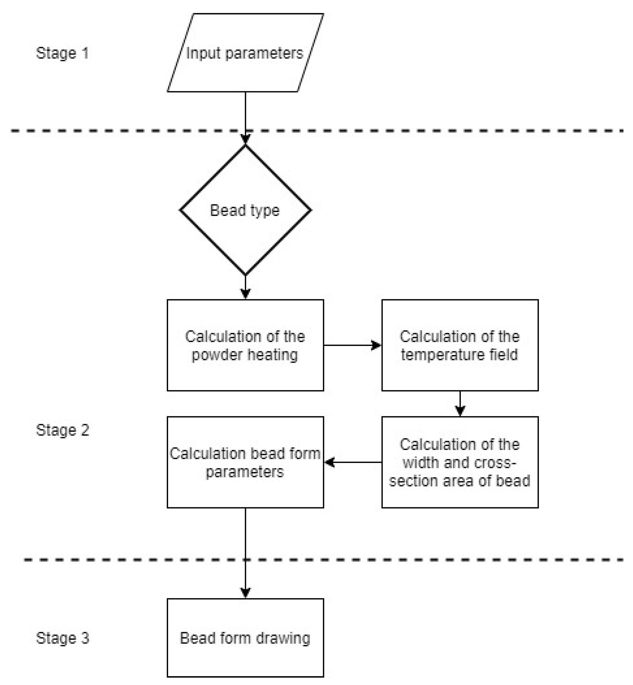
2. Materials and Methods
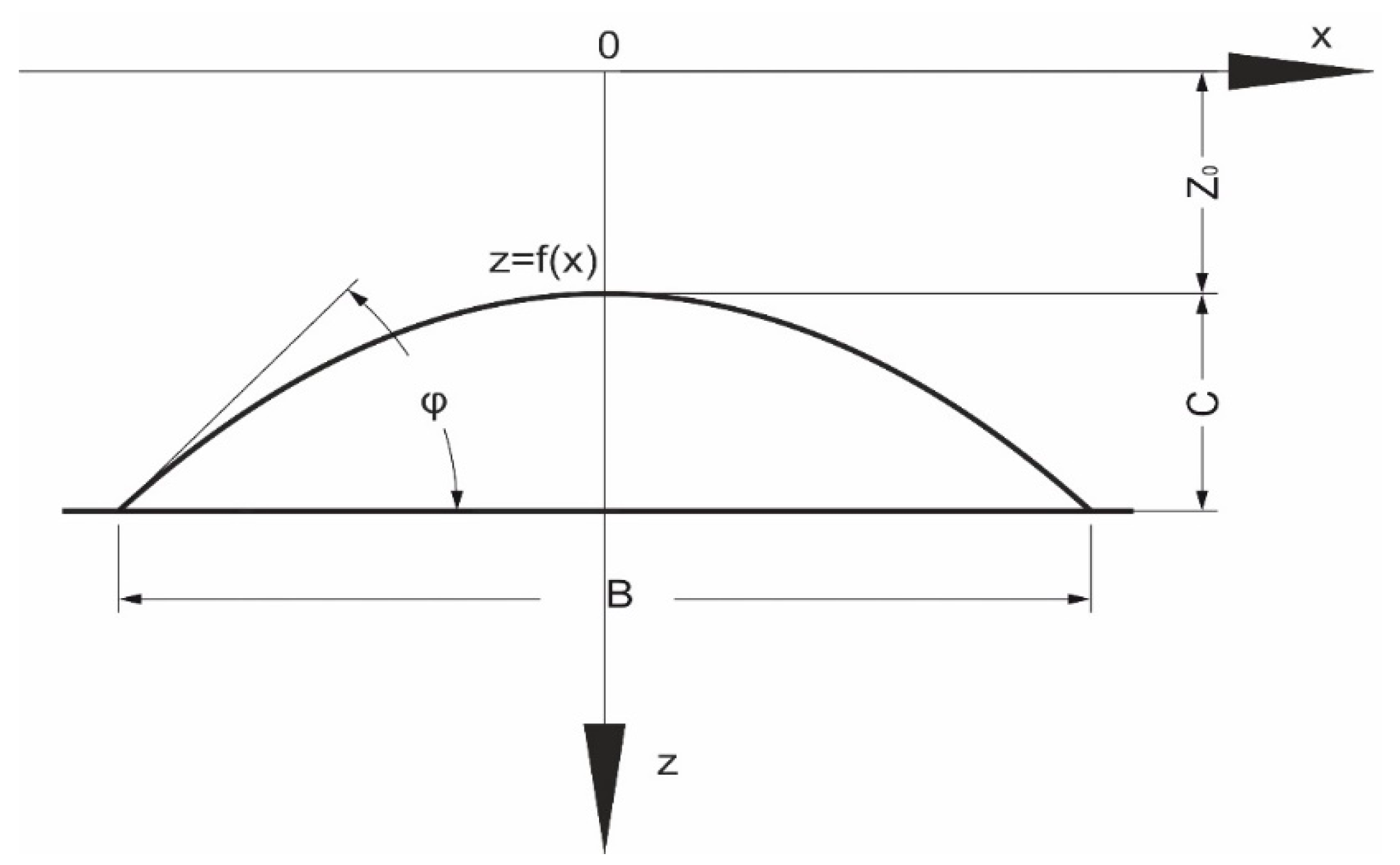
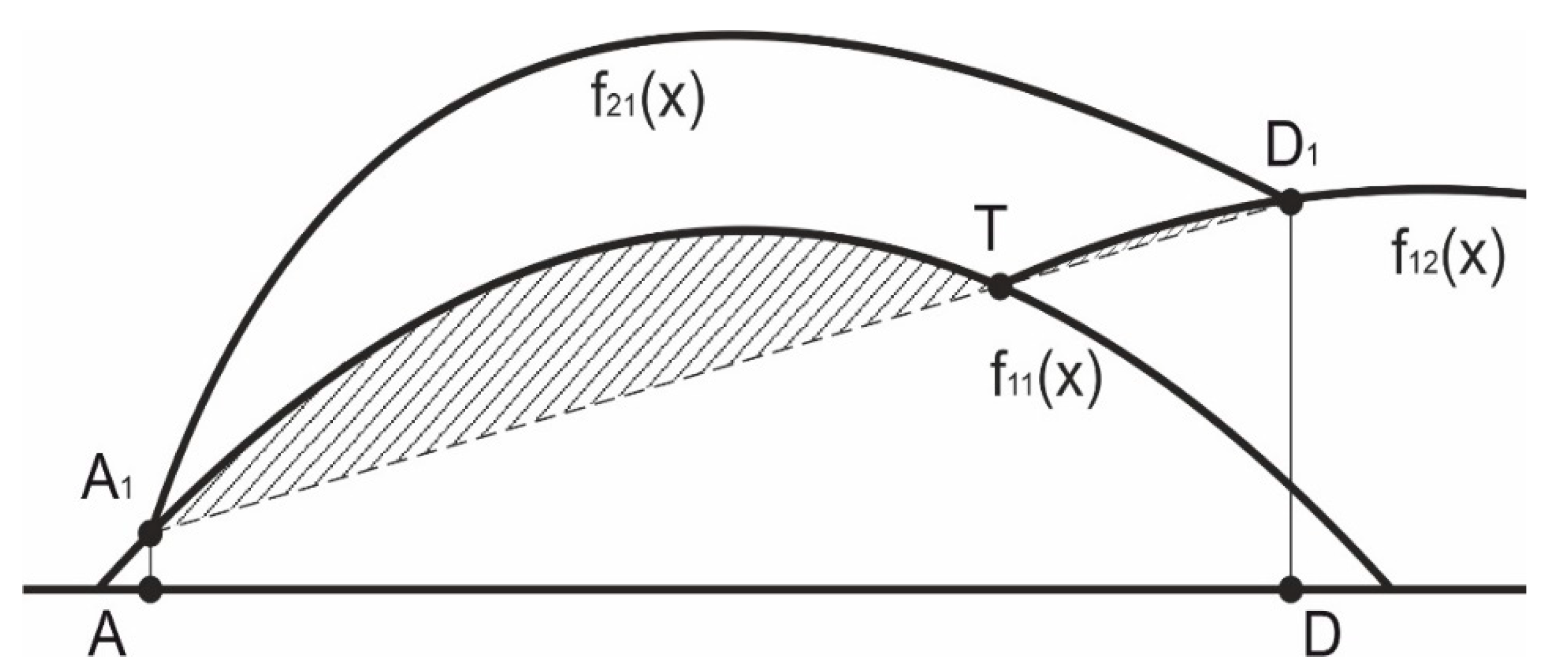
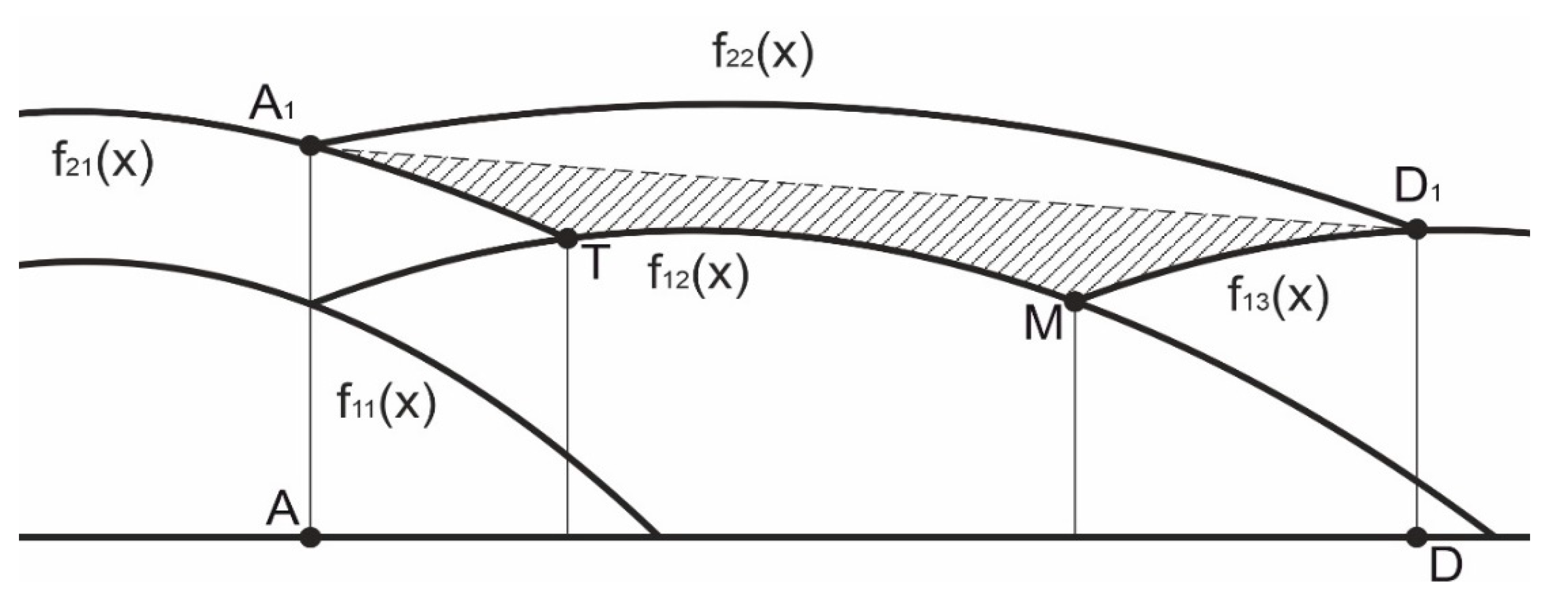
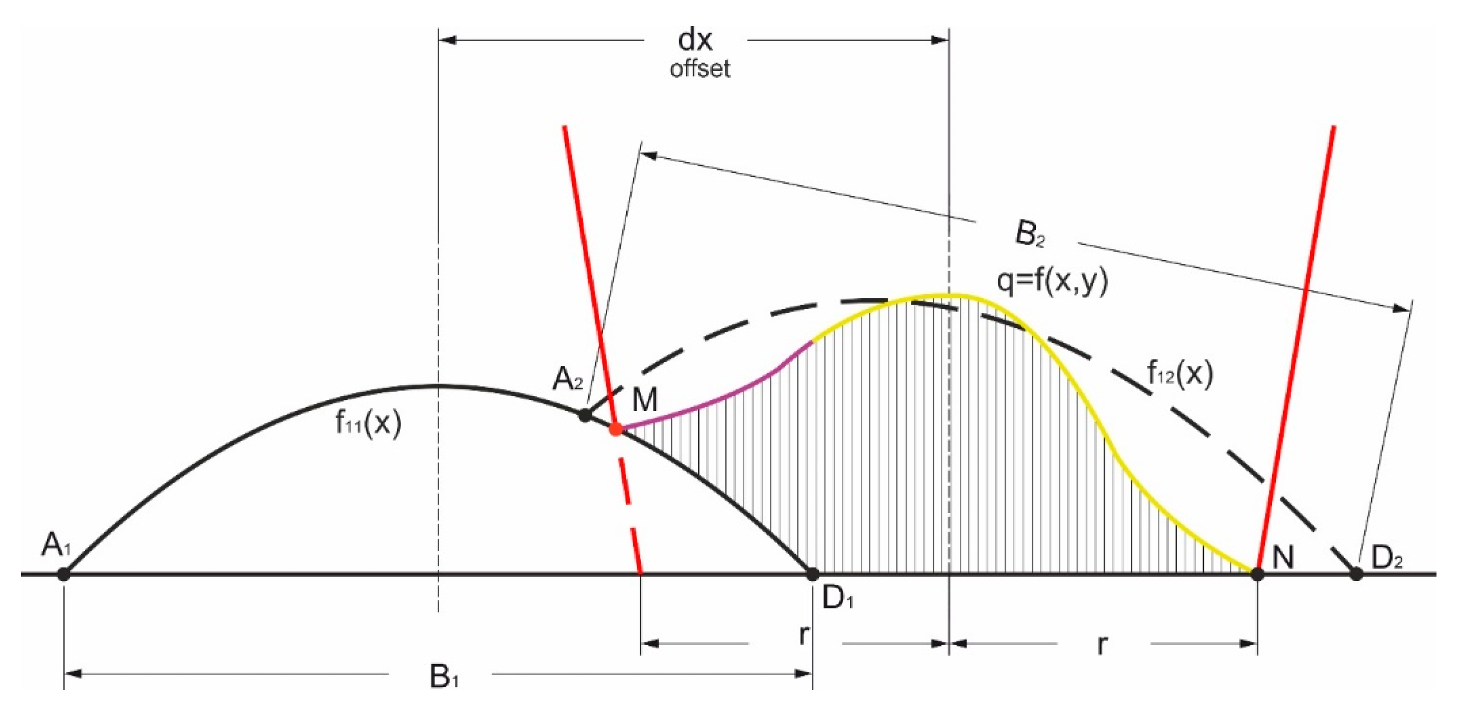
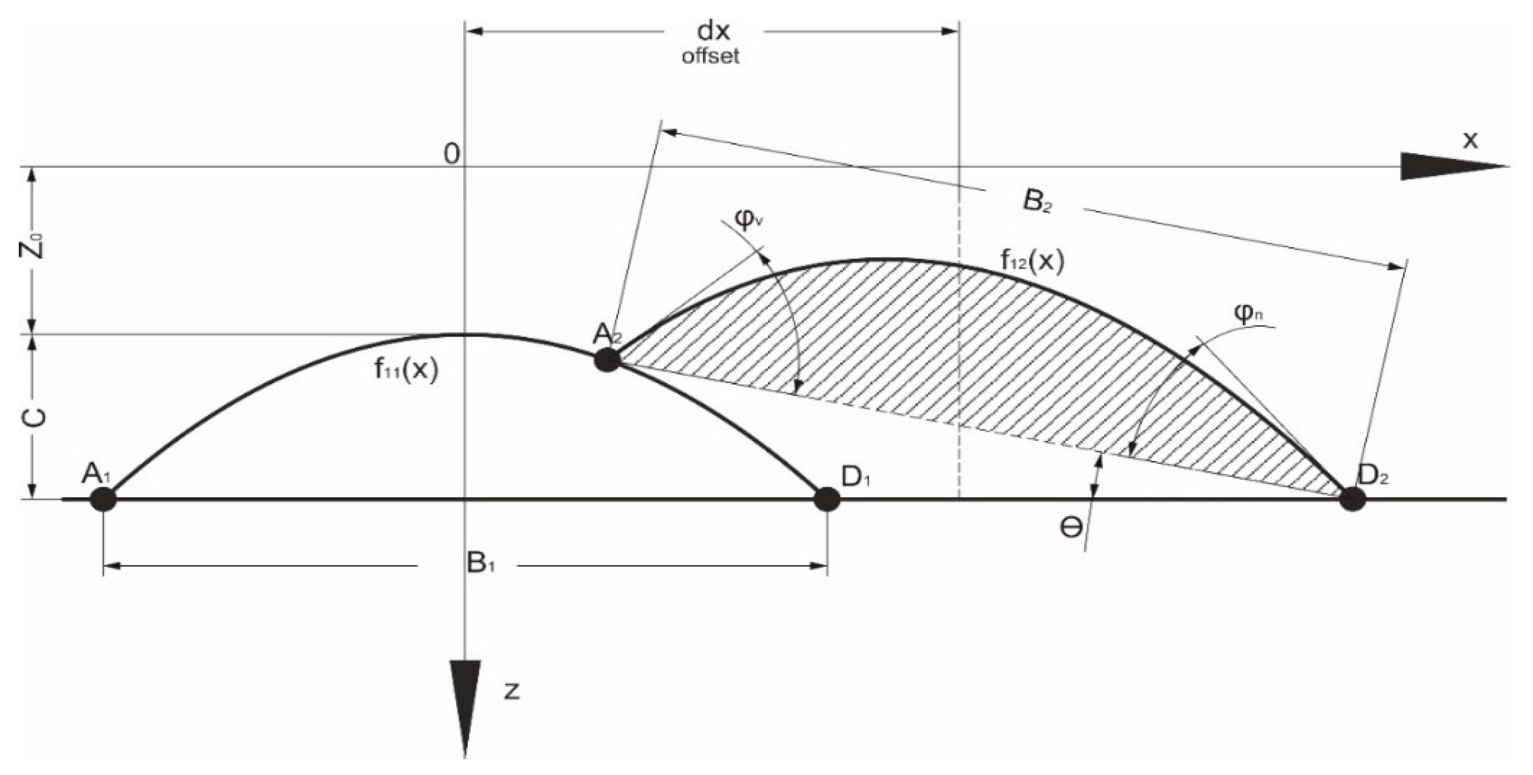
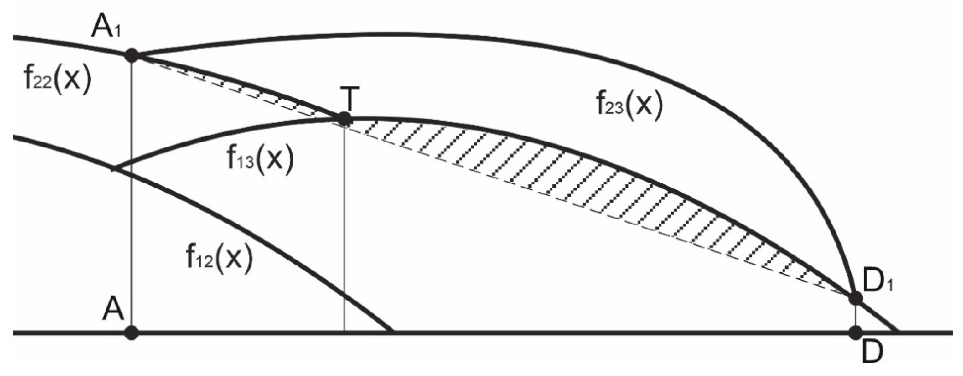
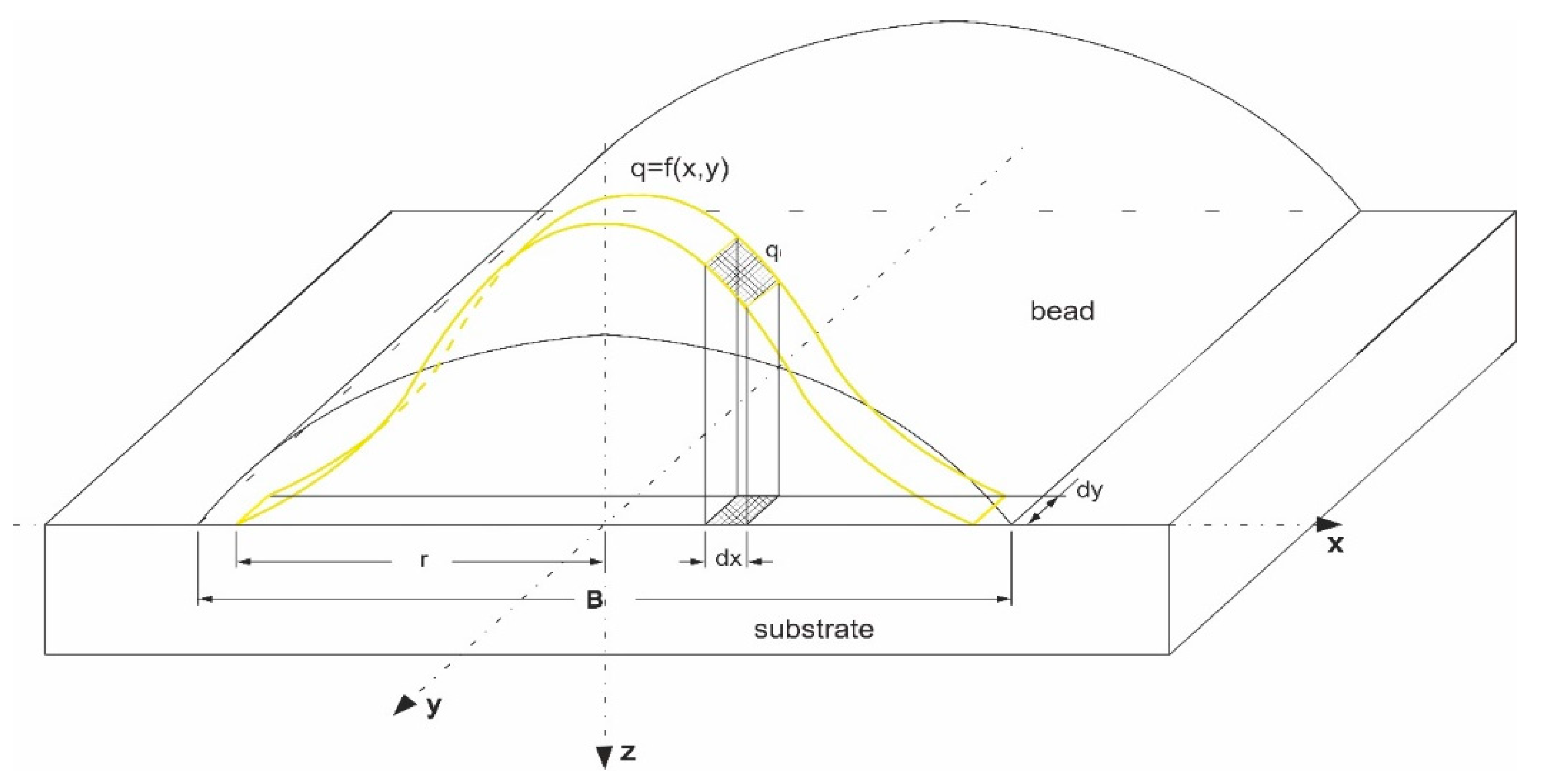
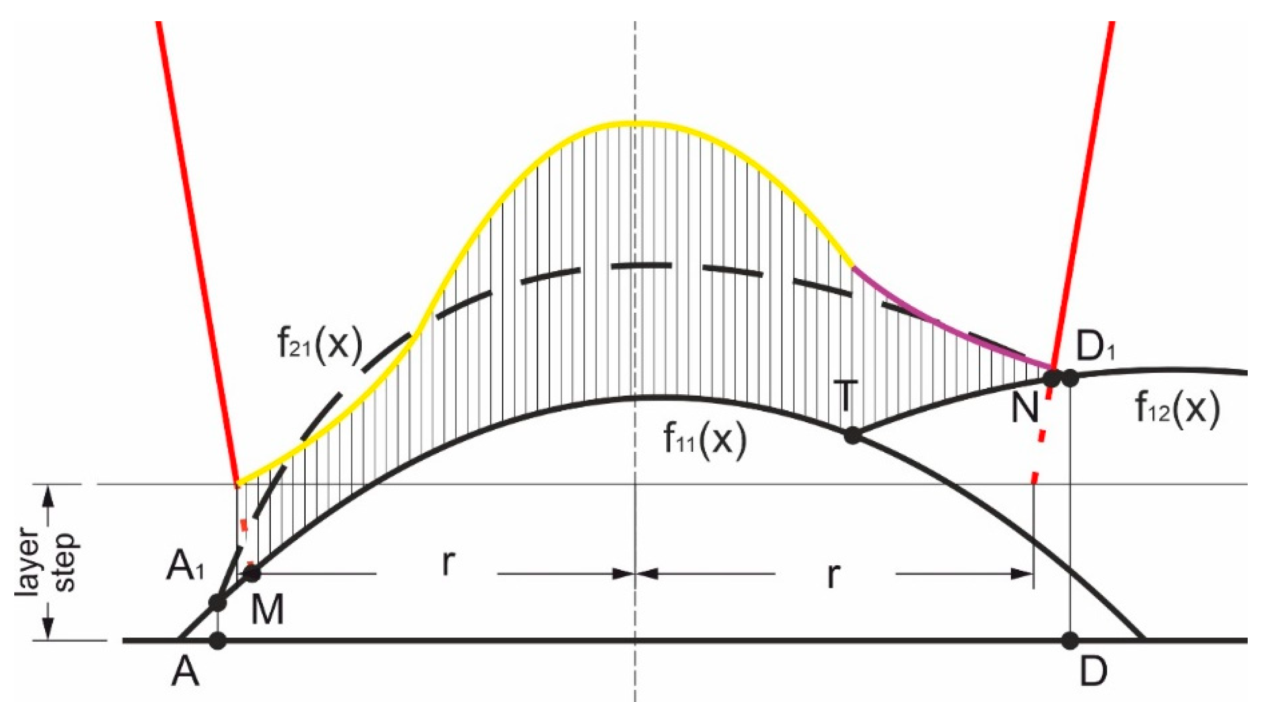
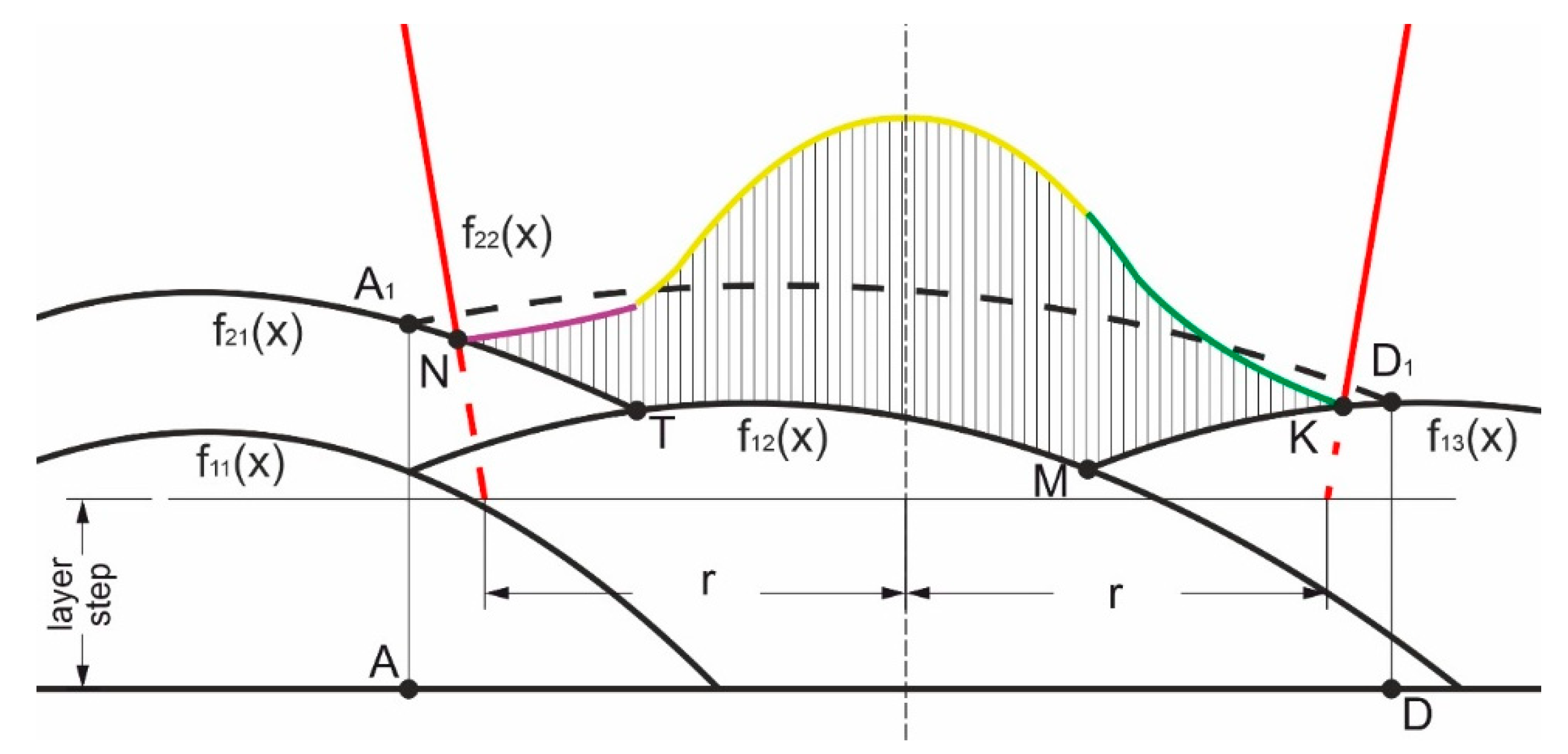
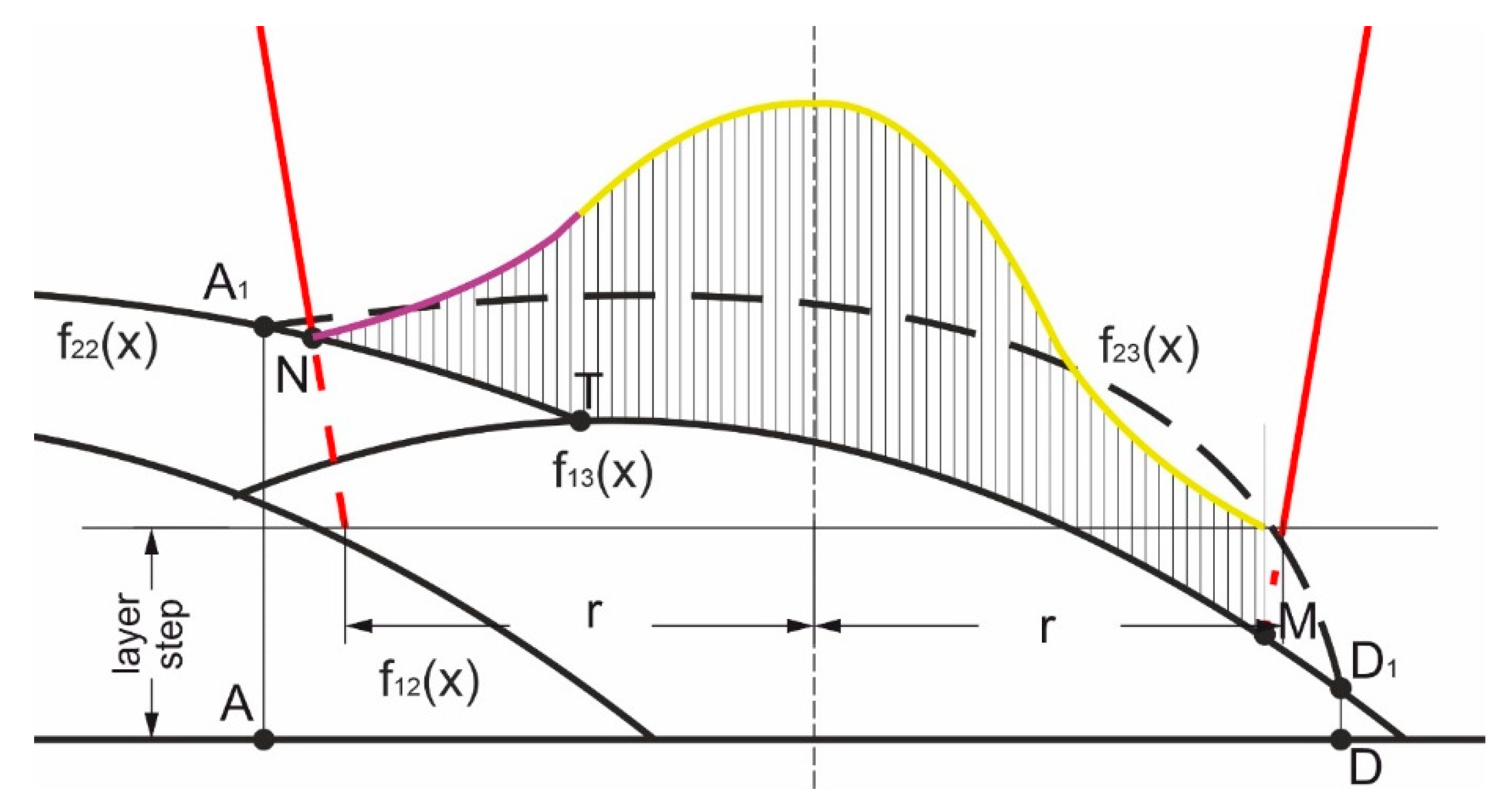
2.1. Bead Formation Description
2.2. Heat Transfer Model
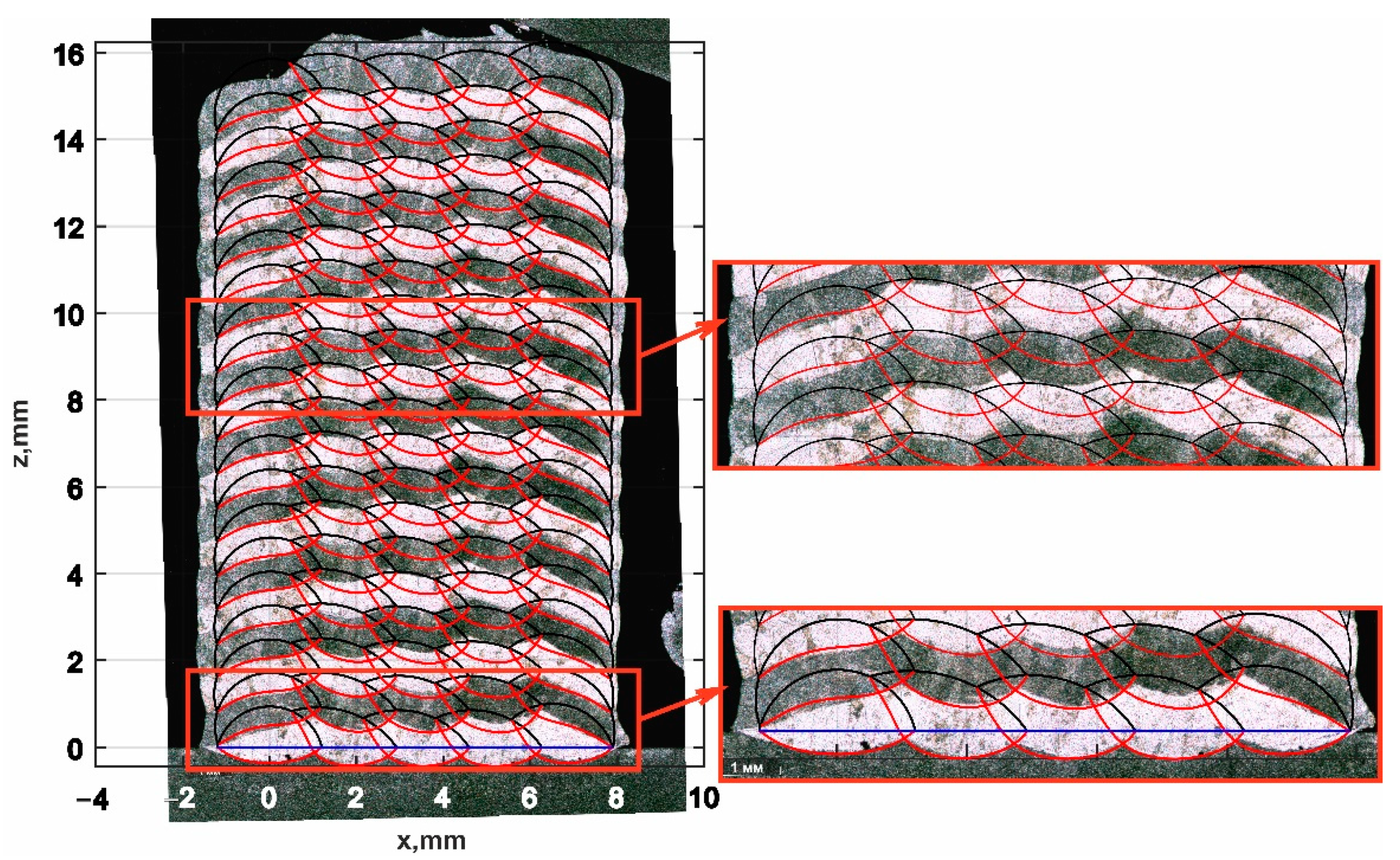
2.3. Experiment Details
3. Results
4. Discussion
5. Conclusions
Author Contributions
Funding
Institutional Review Board Statement
Informed Consent Statement
Data Availability Statement
Conflicts of Interest
References
- Turichin, G.A.; Klimova, G.; Zemlyakov, V.; Babkin, K.D.; Kolodyazhnyy, D.Y.; Shamray, A.; Travyanov, A.Y.; Petrovskiy, P.V. Technological aspects of high speed direct laser deposition based on heterophase powder metallurgy. Phys. Procedia 2015, 78, 397–406. [Google Scholar] [CrossRef] [Green Version]
- Mendagaliyev, R.; Turichin, G.A.; Klimova-Korsmika, O.G.; Zotov, O.G.; Eremeeva, A.D. Microstructure and mechanical properties of laser metal deposited cold-resistant steel for arctic application. Procedia Manuf. 2019, 36, 249–255. [Google Scholar] [CrossRef]
- Magerramova, L.A.; Turichin, G.A.; Nozhnitsky, Y.A.; Klimova-Korsmik, O.G.; Vasiliev, B.E.; Volkov, M.E.; Salnikov, A.V. Peculiarities of additive technologies application in the production of gas turbine engine parts. In Proceedings of the 9th International Conference on Beam Technologies and Laser Application, Saint Petersburg, Russia, 17–19 September 2018. [Google Scholar]
- Rashkovets, M.; Nikulina, A.; Turichin, G.; Klimova-Korsmik, O.; Sklyar, M. Microstructure and phase composition of Ni-based alloy obtained by high-speed direct laser deposition. J. Mater. Eng. Perform. 2018, 27, 6398–6406. [Google Scholar] [CrossRef]
- Turichin, G.; Zemlyakov, E.; Babkin, K.; Ivanov, S.; Vildanov, A. Analysis of distortion during laser metal deposition of large parts. Procedia CIRP 2018, 74, 154–157. [Google Scholar] [CrossRef]
- Korsmik, R.; Tsybulskiy, I.; Rodionov, A.; Klimova-Korsmik, O.; Gogolukhina, M.; Ivanov, S.; Zadykyan, G.; Mendagaliev, R. The approaches to design and manufacturing of large-sized marine machinery parts by direct laser deposition. Procedia CIRP 2020, 94, 298–303. [Google Scholar] [CrossRef]
- Ansari, M.; Martinez-Marchese, A.; Huang, Y.; Toyserkani, E. A mathematical model of laser directed energy deposition for process mapping and geometry prediction of Ti-5553 single-tracks. Materialia 2020, 12, 100710. [Google Scholar] [CrossRef]
- Wang, D.; Li, T.; Shi, B.; Wang, H.; Xia, Z.; Cao, M.; Zhang, X. An analytical model of bead morphology on the inclined substrate in coaxial laser cladding. Surf. Coat. Technol. 2021, 410, 126944. [Google Scholar] [CrossRef]
- Li, J.; Li, H.N.; Liao, Z.; Axinte, D. Analytical modelling of full single-track profile in wire-fed laser cladding. J. Mater. Process. Technol. 2021, 290, 116978. [Google Scholar] [CrossRef]
- Knapp, G.L.; Mukherjee, T.; Zuback, J.S.; Wei, H.L.; Palmer, T.A.; De, A.; DebRoy, T. Building blocks for a digital twin of additive manufacturing. Acta Mater. 2017, 135, 390–399. [Google Scholar] [CrossRef]
- Chai, Q.; Fang, C.; Hu, J.; Xing, Y.; Huang, D. Cellular automaton model for the simulation of laser cladding profile of metal alloys. Mater. Des. 2020, 195, 109033. [Google Scholar] [CrossRef]
- Nie, Z.; Wang, G.; McGuffin-Cawley, J.D.; Narayanan, B.; Zhang, S.; Schwam, D.; Kottman, M.; Rong, Y.K. Experimental study and modeling of H13 steel deposition using laserhot-wire additive manufacturing. J. Mater. Process. Technol. 2016, 235, 171–186. [Google Scholar] [CrossRef]
- Caiazzo, F.; Alfieri, V. Simulation of laser-assisted directed energy deposition of aluminum powder: Prediction of geometry and temperature evolution. Materials 2019, 12, 2100. [Google Scholar] [CrossRef] [PubMed] [Green Version]
- Zhong, C.; Pirch, N.; Gasser, A.; Poprawe, R.; Schleifenbaum, J.H. The influence of the powder stream on high-deposition-rate laser metal deposition with inconel 718. Metals 2017, 7, 443. [Google Scholar] [CrossRef] [Green Version]
- Kovalev, O.; Bedenko, D.; Zaitsev, A. Development and application of laser cladding modeling technique: From coaxial powder feeding to surface deposition and bead formation. Appl. Math. Model. 2018, 57, 339–359. [Google Scholar] [CrossRef]
- Gu, H.; Wei, C.; Li, L.; Han, Q.; Setchi, R.; Ryan, M.; Li, Q. Multi-physics modelling of molten pool development and track formation in multi-track, multi-layer and multi-material selective laser melting. Int. J. Heat Mass Transf. 2020, 151, 119458. [Google Scholar] [CrossRef]
- Panda, B.K.; Sarkar, S.; Nath, A.K. 2D thermal model of laser cladding process of Inconel 718. Mater. Today Proc. 2021, 41, 286–291. [Google Scholar] [CrossRef]
- Wei, H.; Liu, F.; Liao, W.; Liu, T. Prediction of spatiotemporal variations of deposit profiles and inter-track voids during laser directed energy deposition. Addit. Manuf. 2020, 34, 101219. [Google Scholar] [CrossRef]
- Paes, L.E.D.S.; Ferreira, H.S.; Pereira, M.; Xavier, F.A.; Weingaertner, W.L.; Vilarinho, L.O. Modeling layer geometry in directed energy deposition with laser for additive manufacturing. Surf. Coat. Technol. 2021, 409, 126897. [Google Scholar] [CrossRef]
- Liu, J. Formation of cross-sectional profile of a clad bead in coaxial laser cladding. Opt. Laser Technol. 2007, 39, 1532–1536. [Google Scholar] [CrossRef]
- Liu, F.; Wei, L.; Shi, S.; Wei, H. On the varieties of build features during multi-layer laser directed energy deposition. Addit. Manuf. 2020, 36, 101491. [Google Scholar] [CrossRef]
- Karmuhilan, M.; Sood, A.K. Intelligent process model for bead geometry prediction in WAAM. Mater. Today Proc. 2018, 5, 24005–24013. [Google Scholar] [CrossRef]
- Berezovsky, B.M.; Stikhin, V.A. Influence of surface tension forces on the formation of weld reinforcement. Sverochnoe Proizvodstvo (Weld. Prod.) 1977, 1, 51–53. [Google Scholar]
- Matsunawa, A.; Ohji, T. Role of surface tension in fusion welding (Part 1). Trans. JWRI 1982, 11, 145–154. [Google Scholar]
- Berezovsky, B.M. Optimization of metal layer formation during arc surfacing. Weld. Prod. 1990, 6, 33–36. [Google Scholar]
- Berezovsky, B.M.; Stikhin, V.A. Mathematical modeling of the formation of horizontal seams on an inclined plane. Avtom. Svarka (Autom. Weld.) 1988, 1, 26–31. [Google Scholar]
- Korolenko, P.V. Coherent Radiation Optics; Lomonosov Moscow State University Faculty of Physics: Moscow, Russia, 1997. [Google Scholar]
- Li, Z.; Xu, R.; Zhang, Z.; Kucukkoc, I. The influence of scan length on fabricating thin-walled components in selective laser melting. Int. J. Mach. Tools Manuf. 2018, 126, 1–12. [Google Scholar] [CrossRef]
- Sainte-Catherine, C.; Jeandin, M.; Kechemair, D.; Ricaud, J.P.; Sabatier, L. Study of dynamic absorptivity at 10.6 μm (CO2) and 1.06 μm (Nd-YAG) wavelengths as a function of temperature. J. Phys. Proc. EDP Sci. 1991, 1, 151–157. [Google Scholar]
- Kim, S.S. Thermophysical Properties of Stainless Steels; Argonne National Laboratory: Lemont, IL, USA, 1976.
- Xie, J. Laser welding of thin sheet steel with surface oxidation. Weld. J. 1999, 78, 343. [Google Scholar]
- Valencia, J.J.; Quested, P.N. Thermophysical Properties ASM Handbook; Volume 15: Casting; ASM Press: Washington, DC, USA, 2008; pp. 468–481. [Google Scholar]


| No. | Material | Laser Power, W | Velocity, mm/s | Feed Rate, g/min | Beam Diameter, mm | Pause Time, s | ||
|---|---|---|---|---|---|---|---|---|
| First Bead | Mid Bead | Last Bead | ||||||
| 1 | AISI321 | 2000 | 25 | 24.8 | 19.9 | 23.8 | 2.7 | 40 |
| 2 | AISI321 | 2200 | 25 | 24.8 | 19.9 | 23.8 | 2.7 | 40 |
| 3 | AISI321 | 2400 | 25 | 24.8 | 19.9 | 23.8 | 2.7 | 40 |
| 4 | INC718 | 1800 | 25 | 25.8 | 20.6 | 24.7 | 2.7 | 40 |
| 5 | INC718 | 2000 | 25 | 25.8 | 20.6 | 24.7 | 2.7 | 40 |
| 6 | INC718 | 2200 | 25 | 25.8 | 20.6 | 24.7 | 2.7 | 40 |
| 7 | Ti-6Al-4V | 1800 | 20 | 11.2 | 8.9 | 10.7 | 2.3 | 150 |
| 8 | Ti-6Al-4V | 2000 | 20 | 11.2 | 8.9 | 10.7 | 2.3 | 150 |
| 9 | Ti-6Al-4V | 2200 | 20 | 11.2 | 8.9 | 10.7 | 2.3 | 150 |
| 10 | Ti-6Al-4V | 2400 | 20 | 11.2 | 8.9 | 10.7 | 2.3 | 150 |
| No. | Material | Density, g/mm3∙10−6 | Thermal Conductivity, W/(mm∙K)∙10−3 | Specific Heat, J/(g∙K) | Absorption Coefficient | Melting Point, K | Enthalpy, J/g | Surface Tension, J/mm2∙10−3 |
|---|---|---|---|---|---|---|---|---|
| 1 | AISI321 | 7800 | 11.8 | 0.498 | 0.38 | 1723 | 1088 | 1.85 |
| 2 | INC718 | 8190 | 8.9 | 0.435 | 0.23 | 1609 | 1069 | 1.75 |
| 3 | Ti-6Al-4V | 4430 | 8.37 | 0.546 | 0.257 | 1923 | 1575 | 1.33 |
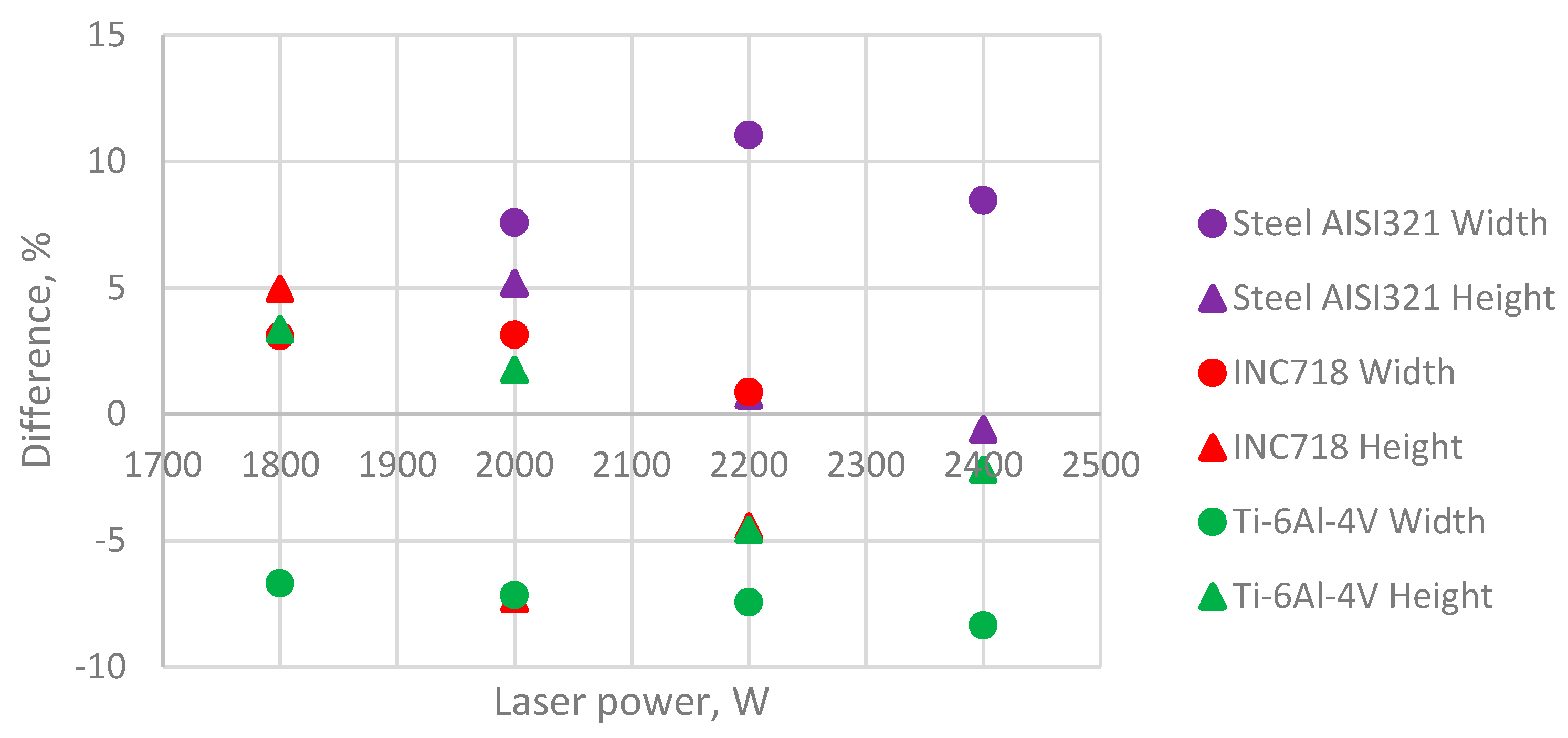
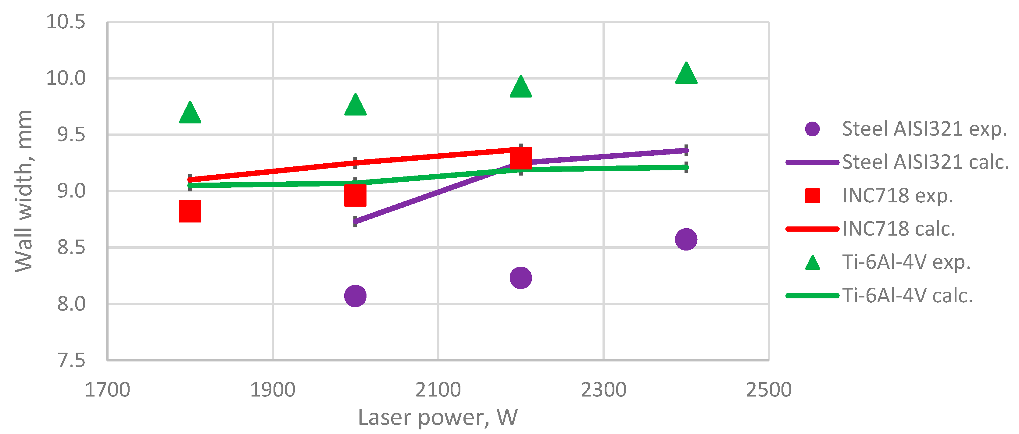
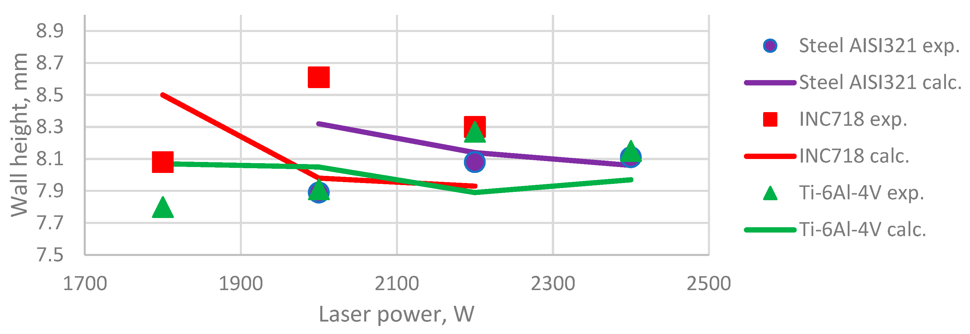
| No. | Material | Height Experimental, mm | Height Calculated, mm | Difference, % | Width Experimental, mm | Width Calculated, mm | Difference, % |
|---|---|---|---|---|---|---|---|
| 1 | AISI321 | 7.89 | 8.32 | 5.17 | 8.07 | 8.73 | 7.56 |
| 2 | AISI321 | 8.08 | 8.14 | 0.74 | 8.23 | 9.25 | 11.03 |
| 3 | AISI321 | 8.11 | 8.06 | −0.62 | 8.57 | 9.36 | 8.44 |
| 4 | INC718 | 8.08 | 8.50 | 4.94 | 8.82 | 9.10 | 3.08 |
| 5 | INC718 | 8.61 | 7.98 | −7.32 | 8.96 | 9.25 | 3.14 |
| 6 | INC718 | 8.30 | 7.93 | −4.46 | 9.29 | 9.37 | 0.85 |
| 7 | Ti-6Al-4V | 7.80 | 8.07 | 3.35 | 9.70 | 9.05 | −6.70 |
| 8 | Ti-6Al-4V | 7.91 | 8.05 | 1.74 | 9.77 | 9.07 | −7.16 |
| 9 | Ti-6Al-4V | 8.27 | 7.89 | −4.59 | 9.93 | 9.19 | −7.45 |
| 10 | Ti-6Al-4V | 8.15 | 7.97 | −2.21 | 10.05 | 9.21 | −8.36 |
Publisher’s Note: MDPI stays neutral with regard to jurisdictional claims in published maps and institutional affiliations. |
© 2021 by the authors. Licensee MDPI, Basel, Switzerland. This article is an open access article distributed under the terms and conditions of the Creative Commons Attribution (CC BY) license (https://creativecommons.org/licenses/by/4.0/).
Share and Cite
Udin, I.; Valdaytseva, E.; Kislov, N. Numerical Estimation of the Geometry of the Deposited Layers during Direct Laser Deposition of Multi-Pass Walls. Metals 2021, 11, 1972. https://doi.org/10.3390/met11121972
Udin I, Valdaytseva E, Kislov N. Numerical Estimation of the Geometry of the Deposited Layers during Direct Laser Deposition of Multi-Pass Walls. Metals. 2021; 11(12):1972. https://doi.org/10.3390/met11121972
Chicago/Turabian StyleUdin, Ilya, Ekaterina Valdaytseva, and Nikita Kislov. 2021. "Numerical Estimation of the Geometry of the Deposited Layers during Direct Laser Deposition of Multi-Pass Walls" Metals 11, no. 12: 1972. https://doi.org/10.3390/met11121972
APA StyleUdin, I., Valdaytseva, E., & Kislov, N. (2021). Numerical Estimation of the Geometry of the Deposited Layers during Direct Laser Deposition of Multi-Pass Walls. Metals, 11(12), 1972. https://doi.org/10.3390/met11121972