Two-Intervals Hardening Function in a Phase-Field Damage Model for the Simulation of Aluminum Alloy Ductile Behavior

Abstract

The aluminum alloys (AA) are among the most utilized materials in engineering structures, which induces the need for careful investigation, testing, and possibilities for accurate simulation of the structure’s response. AA 5083-H111 specimens were used to investigate the possibility of employing a Phase-Field Damage Model (PFDM) for the simulation of AA structures’ behavior. The specimens were mechanically tested by uniaxial tensile loading tests. Based on the obtained results, the PFDM was employed with a von Mises plasticity model, implemented in the Finite Element Method software. The plasticity model was extended by modification of the hardening function defined in two-intervals: a linear hardening and a Simo-type hardening. An excellent superposition of the simulation and experimental force-displacement response was recorded. These findings suggest that the AA structures’ response can be successfully simulated in the elastic-plastic domain, as well as its failure by damage being controlled.

1. Introduction

Although steel is the most represented metal material in engineering structures due to its high strength, Aluminum Alloys (AA) are also strong materials that are opening up possibilities in the engineering design of advanced structures. In exploitation, engineering structures can exhibit non-allowed deformation, which can cause damage of the material and the structure’s collapse. These situations need to be predicted to extend the structure’s life and to increase safety. In studies [1,2,3], numerical and experimental investigation of the materials was the best way to verify the captured results. For that purpose, it is necessary to investigate the material response experimentally and to provide necessary observations for mathematical modeling of the material’s behavior and Finite Element Method (FEM) simulations.

AA5083 is one of the most used AA in the engineering practice (including in shipbuilding, railroad cars, pressure vessels, and aluminum armor), so experimental testing has to be conducted to provide enough information necessary for developing the simulation model. Researchers have widely investigated AA due to its desired mechanical characteristics, such as high strength, being lightweight, and corrosion-resistance, especially in seawater. Recently published articles in scientific journals offer various results on experimental testing and numerical simulation of aluminum alloys. Gao et al. [4] showed, in 2009, that the stress state has strong effects on AA5083 behavior through the experimental and numerical investigation of AA. The results suggest that it is necessary to incorporate hydrostatic stress and the third invariant of the stress deviator in constitutive models. A few years later, Zhou et al., in [5], investigated plastic behavior and a ductile fracture of AA5083 by experimental tests and FEM analyses. They used a specific I1–J2–J3 plasticity model to simulate the plastic response. For the fracture simulation, the failure criterion, based on a damage parameter, was defined. The damage model was local, which took into account the relation between the accumulated plastic strain and the damage state. Darras et al., in [6], investigated the damage state of AA5083 under different loading rates throughout tensile tests at room temperature. They used a scanning electron microscope (SEM) to record the damage at different deformation stages. The energy-based model was utilized to predict isotropic damage values. Lee and Basaran, in [7], offered a review of degradation, damage evolution, and fatigue models for various metals. They discussed various approaches, including, among others, a possibility to simulate the behavior of AA5083 by using the Phase-Field Damage Model (PFDM). One of the latest articles published on this topic in scientific journals is [8]. The degradation of the mechanical characteristics of AA5803 plates was investigated at various temperatures, from room temperature up to 300 °C. It was found that the yield strength did not change up to 150 °C. Furthermore, the temperature influence at the Young modulus was examined, and they concluded that up to 200 °C, the reduction is relatively small (25%). This hot topic has also been covered by Bouhamed et al. in [9]. The possibility of using a coupled plasticity-damage model was presented. It was based on non-associative plasticity equations for simulation of the anisotropic behavior of AA5083. They also investigated the AA5083 material by a uniaxial tensile test. As can be observed in this short literature overview, AA5083 is very interesting to researchers, and many publications have explored its behavior by experimental testing or FEM simulations.

There are various possibilities for the material parameters’ investigation. Christopher et al. [10] investigated the ultimate strength of aluminum composites by advanced techniques, such as neural networks and acoustic emission parameters. Fragassa et al. [11] and Babič et al. [12] also presented machine learning techniques to identify the material parameters. Furthermore, in another article, Fragassa et al. [13] suggested methods for determining the fracture toughness of metallic materials. Dauber et al. [14] correlated the fracture toughness with the erosion resistance to identify fracture mechanisms and cracking in aluminum Al₂O₃. Thus, the material parameters of aluminum alloys are generally interesting for further investigation.

In the previous article by the authors of [1], a fracture phenomenon was explained in detail as cracking of the material for the simulation of steel S355N+J2 structures, which could be simulated by the PFDM. The presented phase-field damage theory is based on the articles of Miehe et al. [15,16,17] and Ambati et al. [18,19,20], which have been well established in the literature. Moreover, all algorithms necessary for easy implementation in the FEM software are available in the previous author’s article [1]. However, in this article, the necessary modifications will be presented along with the theoretical background to show the possibility of using a PFDM coupled with von Mises plasticity, with a modification of the hardening function for the AA5083 behavior simulation.

Two types of metal plasticity constitutive models can be distinguished: micro and macro models. For some specific applications, there is also a combination, known as micro–macro models [21]. The micro models take into consideration the changes in the material at the micro-scale. For that purpose, a deep analysis of the material microstructure is necessary. On the other side, macro (phenomenological) models follow the material’s behavior at a macro-scale, taking into account the material’s response from an engineering point of interest by averaging the micro phenomena. AA5083 specimens cut from a plate used to produce wagons and railroad cars were experimentally investigated. The material parameters were identified to fit the stress-strain response by using the new two-intervals hardening function and comparing the simulation and experimental results. In the end, the experimental testing results and simulation results obtained by the proposed coupling of the PFDM and the von Mises plasticity phenomenological (macro) model and modified two-intervals hardening function were compared, and the verification was successfully done.

In Section 2, the details of the experimental testing are given with the necessary results. The force-displacement responses of uniaxial tensile tests are given as the results of the experimental investigation. Finally, a discussion of the obtained results is given in light of further modifications of the von Mises plasticity hardening function, coupled with thee PFDM.

In Section 3, a short overview of the coupled PFDM–von Mises plasticity approach is repeated to provide the necessary understanding of the stress integration algorithm and iterative procedure and to show a modification of the hardening function for the AA5083 specimens. Furthermore, a comparison of the experimental and simulation results is given as verification of the proposed work.

In Section 4, the main conclusions, along with the main contributions, are presented. In the end, the stress integration algorithm presented in [1] is repeated with appropriate modifications, as seen in Appendix A. Finally, in the Nomenclature section, the nomenclature of the variables used in the algorithms is given.

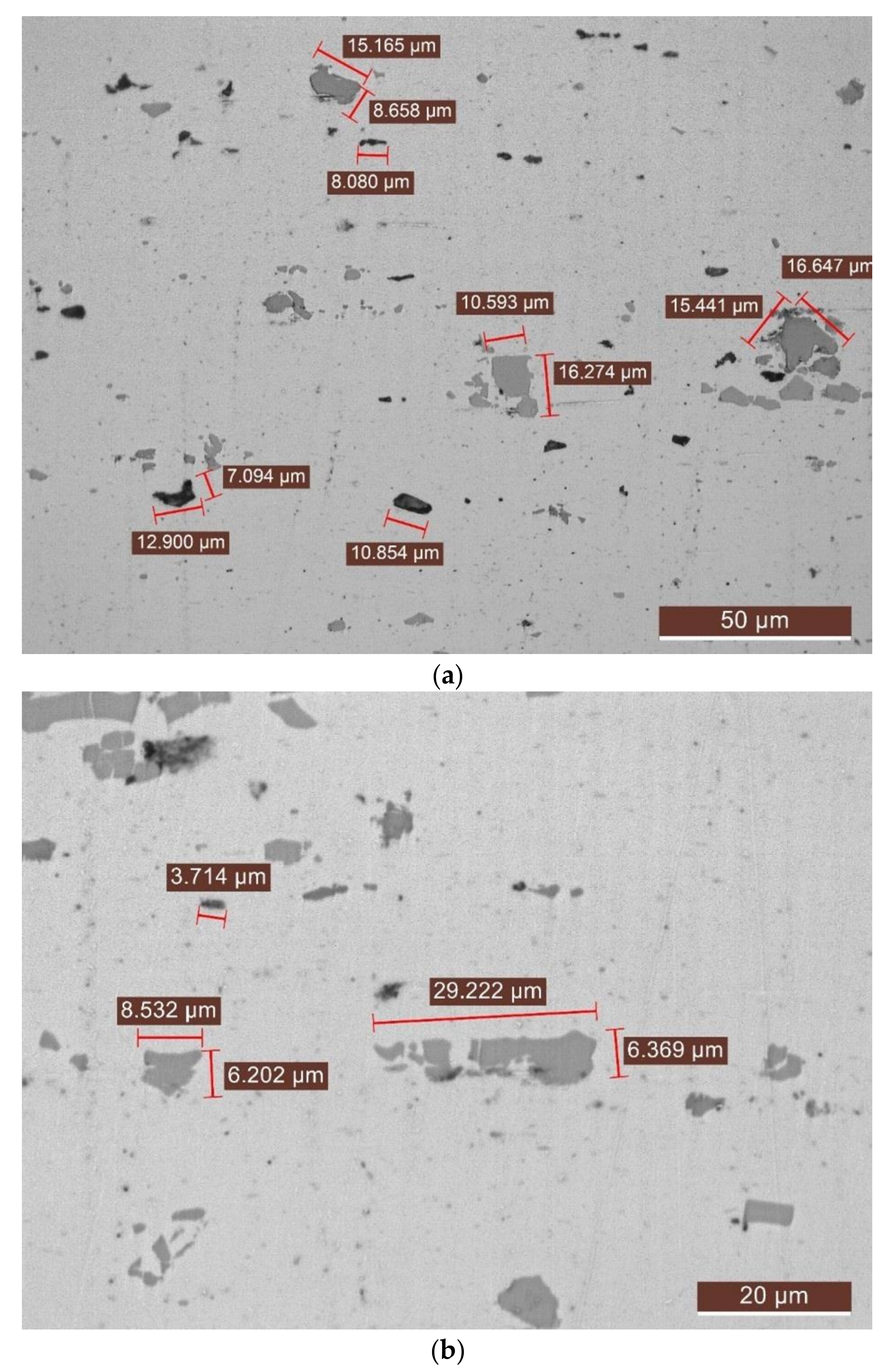
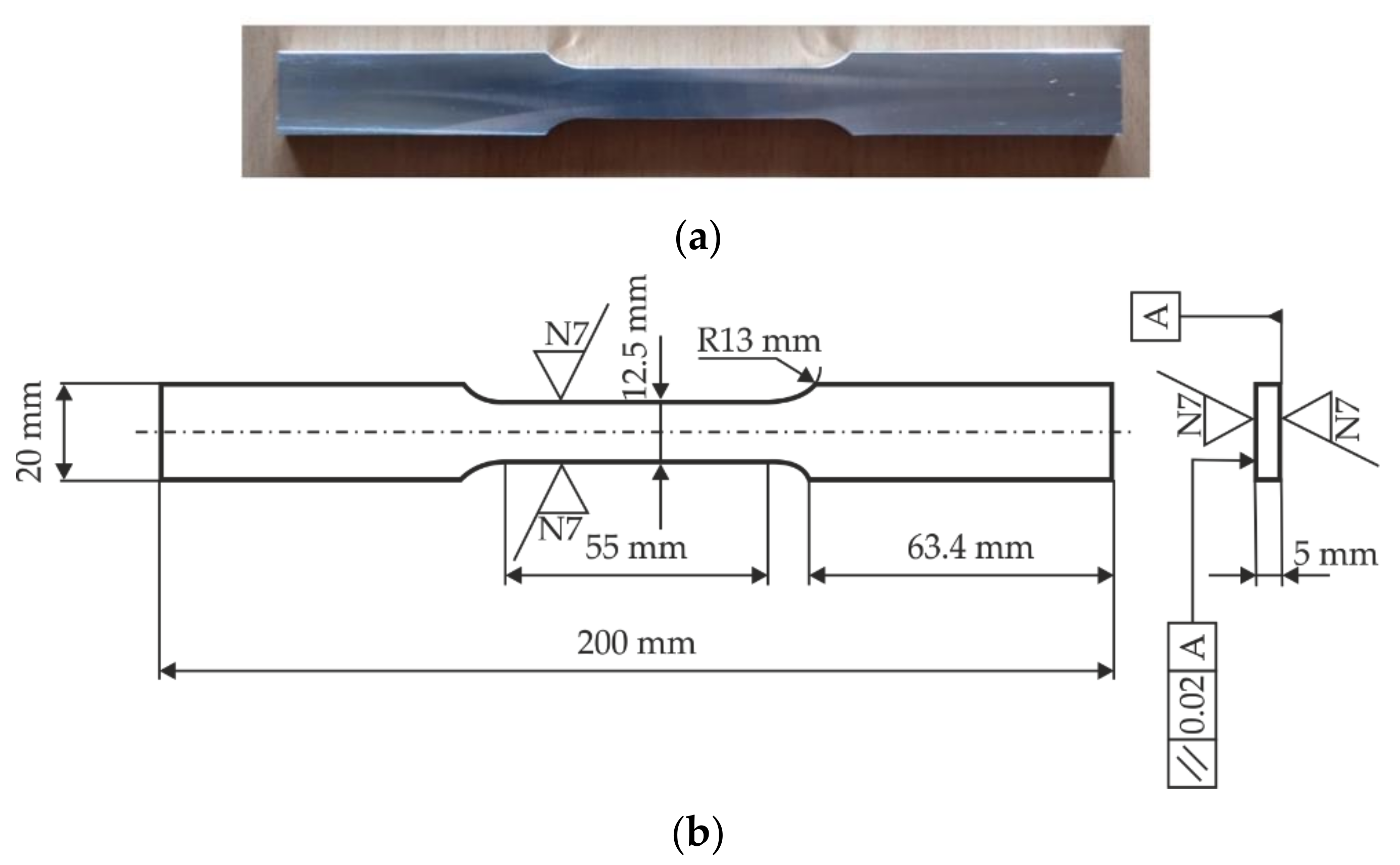
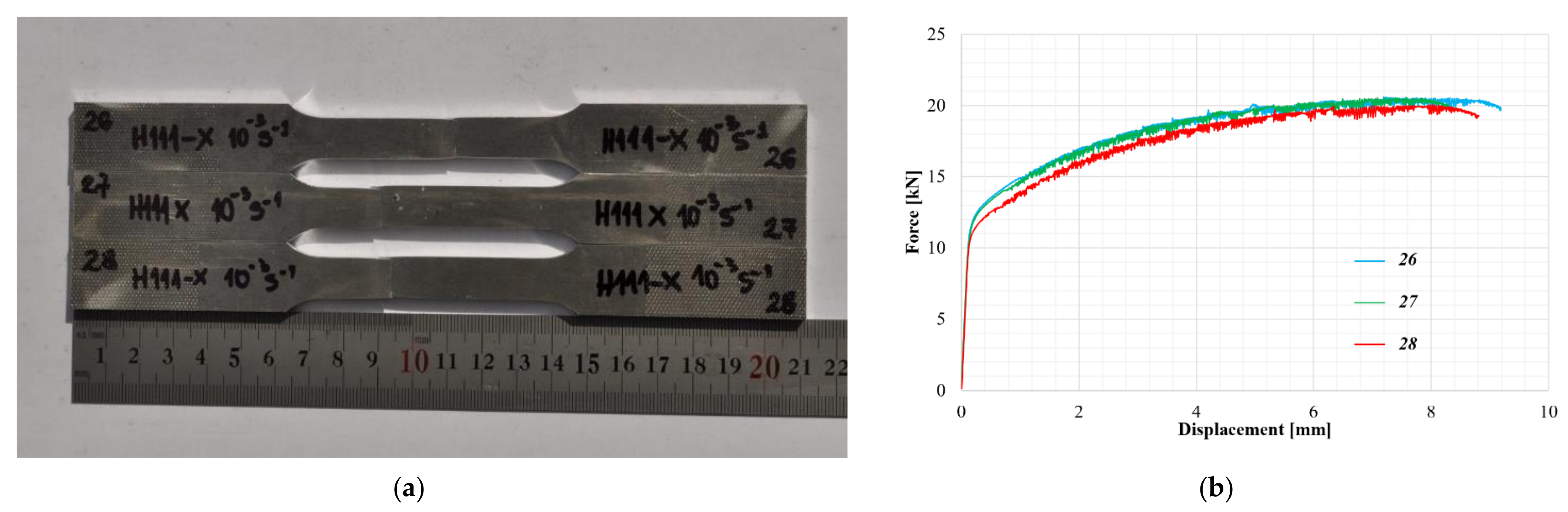
2. Experimental Investigation of AA5083-H111 Specimens

AA5083 has a high corrosion resistance, excellent weldability, and high strength and toughness, and it is used in the naval, automotive, and aerospace industries [22]. It is one of the alloys with the highest strength. It absorbs a lot of energy during fracture, so it is used in situations where high strength is vital.

Specimens required for the static uniaxial tensile tests were cut off from a rolled 8mm thick plate of AA5083-H111. The H111 temper means that the basic material is annealed and slightly strain-hardened. Specimens were mechanically tested on a servo-hydraulic testing machine, EHF-EV101 K3-070-0A (Shimadzu Corporation, Tokyo, Japan), with a force of ±100 kN and stroke of ±100 mm at the Centre for Software Engineering and Dynamical Testing, Faculty of Engineering, University of Kragujevac, Serbia. The chemical composition of the investigated AA5083-H111 from a solid sample was tested on an optical emission spectrometer, SpektroLab LACM12 (SPECTRO Analytical Instruments GmbH, Kleve, Germany), at the IMW Institute Luznice. The obtained values are given in

Table 1. Chemical composition of the examined AA5083-H111 specimens (wt%).

Si	Fe	Cu	Mn	Mg	Cr	Zn	Ti	Al
0.172	0.360	0.036	0.639	4.651	0.074	0.094	0.021	balance

.

The specimen’s microstructure was observed at the IMW Institute by using a LEICA DM4 M specialized metallurgical microscope (Leica microsystems, Wetzlar, Germany). The images from an optical microscope with a magnification of ×500 and ×1000 are given in Figure 1a,b, respectively.

Uniaxial tensile tests were performed on three representative flat specimens (Figure 2a), with the same thickness of all cross-sections, to investigate the material properties. The tests were carried out according to the standard of ASTM E646-00 [23] at room temperature (23 ± 5 °C) for a strain rate of 10⁻³ s⁻¹ (constant stroke control rate of 3 mm/min). The specimen’s shape and dimensions are given in Figure 2b. For the measurement of elongation and identification of Young modulus, the extensometer MFA25 (MF Mess- & Feinwerktechnik GmbH, Velbert, Germany), with a gauge length of 50 mm, was used.

The three investigated AA5083-H111 specimens are presented in Figure 3a (the numbers 26, 27, and 28 written on the specimens were internal markings of the specimens), as well as the recorded force-displacement responses in Figure 3b.

3. Phase-Field Damage Model and von Mises Plasticity for AA5083

The authors of this article have successfully used a PFDM coupled with the von Mises plasticity model to simulate the damage process in S335J2+N steel specimens [1]. It is essential to underline that the constitutive von Mises plasticity model is a macro phenomenological continuum mechanics model, which does not consider the micro-scale behavior of the material. Thus, as it is common in other phenomenological models based on continuum mechanics, the macroscopic variables (damage and equivalent plastic strain) are determined by the appropriate continuum mechanics and thermodynamic laws and rules. The question is whether it is possible to simulate different material responses, such as AA5083, by the same methodology, with appropriate modifications. This research aimed to investigate the AA5083 response by a phase-field damage model coupled with plasticity, by modification of the phenomenological stress-strain hardening curve. For that purpose, in this section, the main details of the PFDM theoretical background will be repeated to explain the necessary changes that are significant for the simulation of AA structures.

The fracture of structures can be considered as a cracking process, which leads to the degradation of the material characteristics. According to Griffith’s theory, the fracture is defined by the equilibrium of the surface energy and the elastic energy. However, this cannot provide a simulation of the crack propagation. For that purpose, the idea of diffuse crack modelling has been established as an interesting solution, which has been successfully used to develop the PFDM. Following Miehe et al. [15,16], Molnár and Gravouil [24], Pañeda et al. [25], and Miehe et al. [26] and appropriate transformations given in [1], the equality of the variation of the internal $\delta \Psi$ and external $\delta W_{ext}$ potential energy can be obtained as follows [1,17,27]:

$$\begin{array}{l}{\displaystyle \underset{V}{\int }\left\{-\left[g^{\prime }\left(d\right)\psi +G_V\left[d-l_c^2{\nabla }^{2}d\right]\right]\delta d\right.}-\left[Div\left[\sigma \right]+b\right]\cdot \delta u+\\ \left.+\left(-g\left(d\right){\sigma }_0:\frac{\partial {\epsilon }_P}{\partial {\overline{\epsilon }}_P}+g\left(d\right){\sigma }_y\right)\delta {\overline{\epsilon }}_P\right\}dV+{\displaystyle \underset{A}{\int }\left\{\left[\sigma \cdot n-h\right]\cdot \delta u\right\}dA+}{\displaystyle \underset{A}{\int }\left\{\left[G_V{l}_c^2\nabla d\cdot n\right]\delta d\right\}dA}=0\end{array}$$

(1)

where $g^{\prime }\left(d\right)$ is the derivative of the degradation function, $g\left(d\right)$, over the damage phase-field variable, $d$; $\psi$ is the internal potential energy density; $G_V$ is the critical fracture energy release rate per unit volume; $l_c$ is the characteristic length-scale parameter; $\nabla$ is the gradient operator; $\sigma$ is the “damaged” Cauchy stress; $b$ is the body force field per unit volume; $u$ is the displacements vector; ${\sigma }_0$ is the Cauchy stress tensor of an undamaged solid; ${\epsilon }_P$ is the plastic strain tensor; ${\overline{\epsilon }}_P$ is the equivalent plastic strain; ${\sigma }_y$ is the yield stress; $n$ is the unit outer, normal to the surface, $A$; and $h$ is the boundary traction per unit area.

By introducing the Neumann-type boundary conditions [1], the equilibrium equation can be derived from Equation (1), as in [1,27]:

$$Div\left[\sigma \right]+b=0,$$

(2)

as well as the phase-field damage evolution law:

$$G_V\left[d-l_c^2{\nabla }^{2}d\right]+g^{\prime }\left(d\right)\psi =0,$$

(3)

and the plasticity yield condition law:

$${\overline{\sigma }}_{eq}-{\sigma }_y=0.$$

(4)

The Formulas (2)–(4) are the main equations that were implemented into the in-house FEM software, PAK, developed at the Faculty of Engineering, University of Kragujevac, Serbia. The large strain plasticity theory [1,20,28,29] has been used to develop the von Mises plasticity stress integration algorithm, which was coupled with the PFDM theory by a multifield 3D finite element.

Ambati et al. [18] defined the coupling degradation function for the PFDM of a ductile fracture as

$$g\left(d\right)={\left(1-d\right)}^{2p}.$$

(5)

In the previous article, [1], the authors proposed a modification of the coupling variable, $p$, to depend on the value of the equivalent plastic strain, ${\overline{\epsilon }}_P$, because the material is considered to be intact (undamaged) until the equivalent plastic strain achieves the critical value, ${\overline{\epsilon }}_P={\overline{\epsilon }}_P^{crit}$. The critical value of the equivalent plastic strain is the value of the plastic strain when the saturation hardening stress is achieved (point C at the Figure 4a). Therefore, the function which defines the coupling variable, $p$, is given as follows:

$$p=\left\{\begin{array}{cc}0& ;{\overline{\epsilon }}_P<{\overline{\epsilon }}_P^{crit}\\ \frac{{\overline{\epsilon }}_P-{\overline{\epsilon }}_P^{crit}}{{\overline{\epsilon }}_P^{crit}}& ;{\overline{\epsilon }}_P\ge {\overline{\epsilon }}_P^{crit}\end{array}\right..$$

(6)

Only the elastic part, ${\psi }_0^E$, is computed as the stored internal potential energy density, $\psi$, because the plastic part is taken into account by the coupling variable, $p$. Furthermore, as it was discussed in [30], it not straightforward which is the best solution. It depends on the type of the material and amount of plastic strain. However, the conclusion is that the contribution of the elastic work is essential and cannot be neglected, so the elastic framework for predicting ductile damage can be used [1,20,30].

The Newton-Raphson iterative procedure has been given in literature [31,32], but for the completeness reason, its staggered variant [1,33] is also presented in this paper. The displacement and damage vector were set to the initial values from the previous time step, $t$, at the beginning [1]:

$$\begin{gathered} u^{\left(0\right)}={}^{t}u, \\ {d}^{\left(0\right)}={}^{t}d. \end{gathered}$$

(7)

The external loads were computed by using the body force field per unit volume, $b$, and the boundary traction per unit area, $h$, as follows [1]:

$$f_e^{ext}={\displaystyle \underset{V}{\int }{\left(N^u\right)}^{T}bdV+}{\displaystyle \underset{A}{\int }{\left(N^u\right)}^{T}hdA},$$

(8)

where $N^u$ is the interpolation matrix for displacements. The loop over the integration points starts by computing the strain-displacement matrix, $B^u$, and the damage matrix, $B^d$. The strain related to displacements and to damage for the $i$-th iteration are [1]:

$${\epsilon }^{\left(i\right)}=B^u{u}^{\left(i\right)}; {\epsilon }^d{}^{\left(i\right)}=B^d{d}^{\left(i\right)}.$$

(9)

Now, for each integration point, the von Mises constitutive model subroutine was employed for stress integration, ${\sigma }_0^{\left(i\right)}$, by the standard radial-return algorithm in plasticity, given in Appendix A.

To implement the staggered Newton-Raphson iterative scheme, the output values from the plasticity model were strain energy, ${\psi }^{\left(i\right)}={}^t\psi$, and the coupling variable, $p^{\left(i\right)}={}^{t}p$, where the upper left index, $t$, denotes the values from the previous time step. The computed stresses, as well as the strain energy and the coupling variable, were then used in the elemental internal forces and the damage residual as [1]:

$$f_e^{\mathrm{int}\left(i\right)}={\displaystyle \underset{V}{\int }g\left(d^{\left(i\right)}\right){\left(B^u\right)}^T{\sigma }_0^{\left(i\right)}dV},$$

(10)

$$r_e^{d\left(i\right)}={\displaystyle \underset{V}{\int }\left\{\left[G_V{d}^{\left(i\right)}-g^{\prime }\left(d^{\left(i\right)}\right){\psi }^{\left(i\right)}\right]{\left(N^d\right)}^T+G_V{l}_c^2{\left(B^d\right)}^T{\epsilon }^d{}^{\left(i\right)}\right\}}dV,$$

(11)

where the damage in an element is computed as $d^{\left(i\right)}=N^d{d}^{\left(i\right)}$, and $N^d$ is the interpolation matrix for the damage phase-field. The components of the stiffness tangent matrices are [1]:

$$K_e^{u\left(i\right)}={\displaystyle \underset{V}{\int }\left\{g\left(d^{\left(i\right)}\right){\left(B^u\right)}^T{C}_{EP}{B}^u\right\}}dV,$$

(12)

$$K_e^{d\left(i\right)}={\displaystyle \underset{V}{\int }\left\{\left[G_V-g^{″}\left(d^{\left(i\right)}\right){\psi }^{\left(i\right)}\right]{\left(N^d\right)}^T\left(N^d\right)+G_V{l}_c^2{\left(B^d\right)}^T\left(B^d\right)\right\}}dV.$$

(13)

The element internal forces and element tangent matrices were then assembled into the global assembly, where a new global displacement and a damage field were computed from the global Newton-Raphson iterations as [1]:

$$\left[\begin{array}{cc}{K}^{u(i)}& 0\\ 0& K^{d(i)}\end{array}\right]\left\{\begin{array}{c}\delta u\\ \delta d\end{array}\right\}=\left\{\begin{array}{c}{f}^{\mathrm{ext}}\\ 0\end{array}\right\}-\left\{\begin{array}{c}{f}^{\mathrm{int}(i)}\\ r^{d(i)}\end{array}\right\},$$

(14)

$$u^{\left(i+1\right)}=u^{\left(i\right)}+\delta u; \hspace{1em}\hspace{1em}\hspace{1em} d^{\left(i+1\right)}=d^{\left(i\right)}+\delta d.$$

(15)

If convergence criteria $‖f^{\mathrm{ext}}-f^{\mathrm{int}(i)}‖\le tol$ and $‖r^{d\left(i\right)}‖\le tol$ are satisfied, one can proceed to next time step.

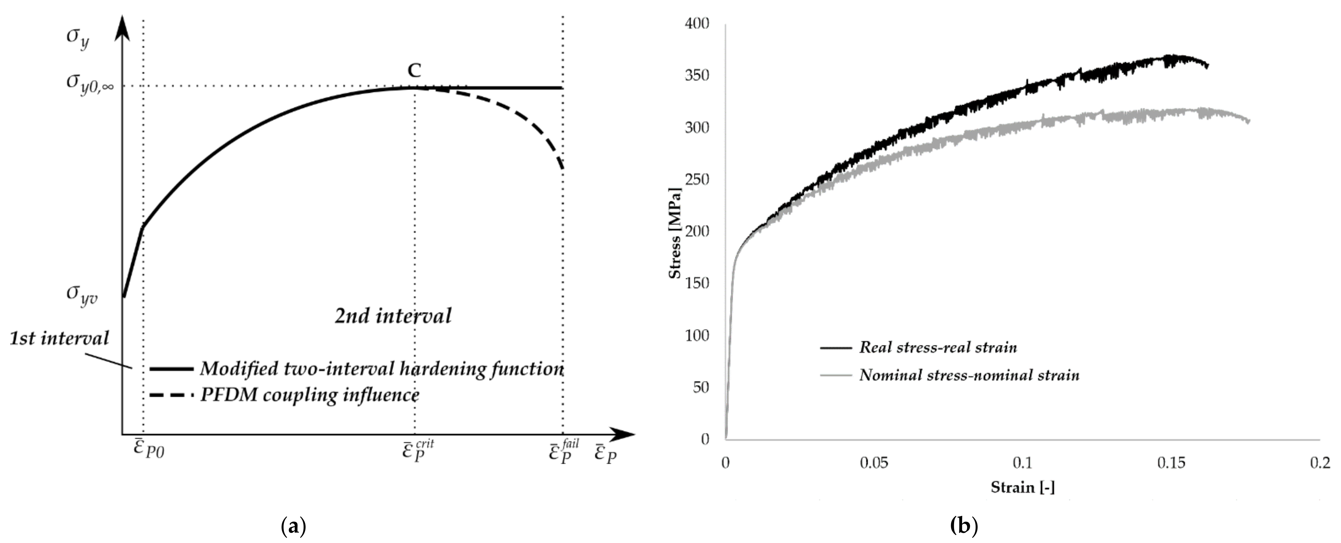
3.1. Short Overview of the von Mises Plasticity and Modifications of Two-Intervals Hardening Function for AA5083 Structures

The idealized response of AA5083 is given in Figure 3a (continuous line). As can be noticed, the yielding occurred after the initial yield stress, ${\sigma }_{yv}$, was achieved. The main new observation, which needed to be considered and implemented in this model with respect to the literature [1], was divided in the two intervals. In the first interval, when the plastic strain increased, the stress increased suddenly for the small plastic strain increment, so that it could be idealized by linear hardening (${\overline{\epsilon }}_P<{\overline{\epsilon }}_{P0}$), defined by the linear hardening function, $H_0$. The previous hardening function, presented in [1], considered this interval by perfect plasticity (no hardening). Thus, in the first interval, the yield condition is given in the following form [22]:

$$f_y={\overline{\sigma }}_{eq}-\left({\sigma }_{yv}+H_0{\overline{\epsilon }}_P\right)\le 0.$$

(16)

From the diagram in Figure 4a, it can be seen that stress increased nonlinearly in the second interval until the saturation hardening stress, ${\sigma }_{y0,\infty }$, was achieved. The response could be covered by Simo hardening function, previously used in literature [1,29], as

$$f_y={\overline{\sigma }}_{eq}-\left[{\sigma }_{yv}+\left({\sigma }_{y0,\infty }-{\sigma }_{yv}\right)\left(1-e^{-n\left({\overline{\epsilon }}_P-{\overline{\epsilon }}_{P0}\right)}\right)+H\left({\overline{\epsilon }}_P-{\overline{\epsilon }}_{P0}\right)\right]\le 0.$$

(17)

When the saturation hardening stress, ${\sigma }_{y0,\infty }$, was achieved, the stress decreased, due to the damage of the material and degradation of the material parameters. This segment could be captured by the PFDM (dashed line).

The complete two-intervals yield function, shown in Figure 4a by a continuous line, can be defined by the following Equation (4):

$$f_y={\overline{\sigma }}_{eq}-{\overline{\sigma }}_y,$$

(18)

where we suggest modification of the yield stress function as

$${\sigma }_y=\left\{\begin{array}{cc}{\sigma }_{yv}+H_0{\overline{\epsilon }}_P& ;{\overline{\epsilon }}_P<{\overline{\epsilon }}_{P0}\\ {\sigma }_{yv}+\left({\sigma }_{y0,\infty }-{\sigma }_{yv}\right)\left(1-e^{-n\left({\overline{\epsilon }}_P-{\overline{\epsilon }}_{P0}\right)}\right)+H\left({\overline{\epsilon }}_P-{\overline{\epsilon }}_{P0}\right)& ;{\overline{\epsilon }}_P\ge {\overline{\epsilon }}_{P0}\end{array}\right..$$

(19)

The yield Function (18) was less than zero for the elastic solution, but if $f_y>0$, the equivalent plastic strain increment of the function, $f_y\left(\Delta {\overline{\epsilon }}_P\right)=0$, must be determined in an iterative procedure given in Appendix A [1].

3.2. Verification of the Proposed Two-Intervals Yield Function Modification

To verify the coupling between the PFDM and von Mises plasticity algorithm, described in detail in [1], with the proposed modifications of the two-intervals hardening function for simulation of AA5083 specimens, the FE model was prepared for the straight part of the specimen. The length of the model was the same as the gauge length (h + l = 50 mm). Because the model had three symmetry planes, it was possible to prescribe proper boundary conditions and to model only one-eighth of the specimen (25 mm × 6.25 mm × 2.5 mm). The plastic deformation was triggered by imperfection in the specimen, which also should have been prescribed in the model. The geometrical imperfection has been proposed in Figure 5, in the zone of 10 mm (l) from the middle of the specimen, as 0.01%, representing a linear decrease of the specimen width, $d$, and thickness. The decrease of the geometry dimensions is presented by a different greyscale. The imperfection was chosen as the smallest defect of specimens that could be observed during the production process. In the experimental investigation, the specimen defect was one of the factors that was responsible for the initiation of the damage zone in the material.

Because the von Mises plasticity constitutive model for large strain problems considers the relation between Cauchy stress and logarithmic (Hencky) strain, the material parameters were estimated for the real stress–real strain experimental response. The nominal stress, ${\sigma }_0$, and the nominal strain, $\epsilon$, were calculated as

$${\sigma }_0=\frac{F}{A_0}, \hspace{1em}\hspace{1em} \epsilon =\frac{\Delta l_g}{l_{g0}},$$

(20)

where $F$ is the loading force measured by the universal testing machine, $A_0$ is the nominal cross-section area of the specimen, $\Delta l_g$ is the displacement measured by the extensometer, and $l_{g0}$ is the nominal gauge length. The real stress, $\sigma$, and the real strain, $h$, were than calculated as

$$\sigma ={\sigma }_0\left(1+\epsilon \right), \hspace{1em}\hspace{1em} h=\ln \left(1+\epsilon \right).$$

(21)

The estimated parameters are given in

Table 2. Material parameters used in PFDM simulation.

$\mathit{E}\left[\mathbf{MPa}\right]$	$\mathit{\nu }\mathbf{[}\mathbf{-}\mathbf{]}$	${\mathit{\sigma }}_{\mathit{y}\mathit{v}}\mathbf{\left[}\mathbf{MPa}\mathbf{\right]}$	${\mathit{\sigma }}_{\mathit{y}\mathbf{0},\mathbf{\infty }}\mathbf{\left[}\mathbf{MPa}\mathbf{\right]}$	$\mathit{H}\mathbf{\left[}\mathbf{MPa}\mathbf{\right]}$	$\mathit{n}\mathbf{[}\mathbf{-}\mathbf{]}$	${\mathit{G}}_{\mathit{V}}\mathbf{\left[}\mathbf{MPa}\mathbf{\right]}$	${\mathit{l}}_{\mathit{c}}\mathbf{\left[}\mathbf{mm}\mathbf{\right]}$	${\overline{\mathit{e}}}_{\mathit{P}}^{\mathit{c}\mathit{r}\mathit{i}\mathit{t}}\mathbf{[}\mathbf{-}\mathbf{]}$	${\overline{\mathit{e}}}_{\mathit{P}\mathbf{0}}\mathbf{[}\mathbf{-}\mathbf{]}$	${\mathit{H}}_{\mathbf{0}}\mathbf{\left[}\mathbf{MPa}\mathbf{\right]}$
69.0	0.33	137.63	370.25	103.26	15.99	5.66	0.01	0.14	0.0017	24642.41

as $E \left[\mathrm{MPa}\right]$: Young’s modulus, $\nu [-]$: Poisson’s ratio, ${\sigma }_{yv}\left[\mathrm{MPa}\right]$: initial yield stress, ${\sigma }_{y0,\infty }\left[\mathrm{MPa}\right]$: saturation hardening stress, $H \left[\mathrm{MPa}\right]$: hardening modulus, $n [-]$: hardening exponent, $G_V \left[\mathrm{MPa}\right]$: fracture energy release rate, $l_c\left[\mathrm{mm}\right]$: characteristic length, ${\overline{e}}_P^{crit}$: critical equivalent plastic strain, ${\overline{e}}_{P0}$: linear hardening plasticity equivalent plastic strain, and $H_0 \left[\mathrm{MPa}\right]$: linear hardening modulus. It is evident that after the yield stress was achieved, the stress increased suddenly due to the work hardening process. After the plastic strain increased enough, the stress became the maximal value, considered as saturation hardening stress. At the end of the loading process, the stress decreased, and the fracture occurred. By reading the stress-strain diagram in Figure 4b, the majority of the material parameters could be determined by reading the real stress–real strain curve, but a few of them needed to be obtained in a calibration process (execution of the simulation and comparison of the obtained results to the experimental response). The material parameters of the hardening function (${\sigma }_{yv}$, ${\sigma }_{y0,\infty }$, $H$, $n$, ${\overline{e}}_{P0}$, $H_0$) used for the simulations were calibrated by reading the real stress-strain diagram and fitting the curve by the least squares method. The phase-field parameters ($G_V$, $l_c$) were calibrated in an iterative process by execution of the simulation and comparison of the obtained results with the experimental response. The critical equivalent plastic strain (${\overline{e}}_P^{crit}$), which is related to the coupling variable, $p$, was estimated from the stress-strain diagram as the value of the plastic strain when the loading attained the saturation hardening stress.

As the first choice, the FE model tensile loading was applied to the top surface nodes by a displacement increment of 0.02 mm for 350 steps. Figure 6 shows the dependence between the damage field and the equivalent plastic stress field obtained by the PDFM, so it can be concluded that the leading cause of the specimen’s fracture was the occurrence of damage. Figure 6a shows the equivalent plastic strain field for plasticity without a phase field, and Figure 6b shows the PFDM simulation, so that the influence of the damage field on the localization of plastic strains can be observed. Figure 6a shows the plastic strain field distributed along with the model, with a minimum difference between the minimum and maximum value, while the damage field distribution given in Figure 6c corresponds to the equivalent plastic strain field in Figure 6b, so that it could be considered a generator of the fracture process. The similar character of the damage field and equivalent plastic strain field given in Figure 6b,c was the result of the dependence between the stiffness degradation function (5) and the coupling variable (6), which is dependent on the equivalent plastic strain amount. The coupling variable, $p$, was responsible for the noted correlation.

The comparison of the force-displacement relationship between the experimental and simulation (PFDM + plasticity and “pure” von Mises plasticity) results is given in Figure 7. As can be noticed, the “pure” von Mises plasticity model, denoted as “Plasticity”, could not follow the experimental curve after the loading force attained the maximum value. For the correct simulation of the material response, the PFDM was activated, and the curve denoted as “PFDM + plasticity” could reproduce the experimental response. By the comparison of the computational time necessary for the simulation of “pure” plasticity and “PFDM + plasticity”, it was revealed that PFDM is approximately 70% more expensive, which could be considered as an acceptable difference. Although the numerical results obtained by using the PFDM approach could not simulate the serrated flow in all three experimental curves, the numerical and experimental curves were generally in good agreement. The experimental investigation results were recorded by using the strain gauge and the universal testing machine. When the degradation evolved, the fracture suddenly occurred, which interrupted the recording of the experimental investigation. However, the simulation results were obtained by using the quasi-static analysis, which revealed the possible behavior of the material beyond that point. For more sophisticated measuring devices and smaller loading rates, it would probably be possible to record the experimental response which should be similar to the simulation results. The significance of this comparison is essential for both simulations and experiments in future work.

As it was discussed in [33], the staggered solution scheme was not unconditionally stable. Furthermore, in this work, the sensitivity to the size of the displacement increment used for the simulation is shown by a study given in Figure 8. It can be noticed that the simulated response in the softening zone depends on the increment size, so the behavior after the fracture point is not considered as unique by using this approach. The force–displacement result differs in the softening region in the examples presented in [33], which was also verified in this case.

Firstly, the coarse FE mesh, with a uniform element length of 1 mm, was investigated (1 mm in Figure 9). The FE mesh was than refined along the $l$ length zone, so that the element’s dimension along the specimen length was 0.5 mm in that zone (0.5 mm in Figure 9). The elements were than reduced four times in the first two rows (the element length was 0.125 mm in Figure 9) and 10 times (the element length was 0.05 mm in Figure 9). It can be noticed that the mesh with the smallest dimension of the elements (0.05 mm) had the softest response in the zone of the material degradation [20]. The evolution of the damage field for the post-critical behavior is given in Figure 10. The damage field evolved in the necking zone of the specimen, up to the value which maintained stability of the computational algorithm. For further simulation after the fracture occurred, it is necessary to implement an element “death”, which is planned in future work.

4. Conclusions

The PFDM was successfully used for the simulation of steel structures coupled with plasticity models in previous research by the authors [1]. This provided the idea to apply the same approach to aluminum alloys. The most utilized AA5083 was first experimentally investigated by uniaxial tension tests. The observations of the force-displacement and the stress-strain responses and the literature results were used to identify the material parameters and to propose modifications of the yield hardening function. The two-intervals (linear plus Simo-type hardening) yield function was modified to fit the AA5083 response. The successful implementation of the modified two-intervals hardening function was verified by comparison to the experimental results for AA5083–H111. An excellent superposition was obtained for the force-displacement response. These findings suggest that the PFDM coupled with von Mises plasticity can be used for the simulation of the material response and the damage propagation for various metals, including AA, with minimal modifications of the hardening function.

References

1. Živković, J.; Dunić, V.; Milovanović, V.; Pavlović, A.; Živković, M. A Modified Phase-Field Damage Model for Metal Plasticity at Finite Strains: Numerical Development and Experimental Validation. Metals 2021, 11, 47. [Google Scholar] [CrossRef]
2. Dunić, V.; Pieczyska, E.A.; Kowalewski, Z.L.; Matsui, R.; Slavković, R. Experimental and Numerical Investigation of Mechanical and Thermal Effects in TiNi SMA during Transformation-Induced Creep Phenomena. Materials 2019, 12, 883. [Google Scholar] [CrossRef] [Green Version]
3. Dunić, V.; Pieczyska, E.; Tobushi, H.; Staszczak, M.; Slavković, R. Experimental and numerical thermo-mechanical analysis of shape memory alloy subjected to tension with various stress and strain rates. Smart Mater. Struct. 2014, 23, 055026. [Google Scholar] [CrossRef]
4. Gao, X.; Zhang, T.; Hayden, M.; Roe, C. Effects of the stress state on plasticity and ductile failure of an aluminum 5083 alloy. Int. J. Plast. 2009, 25, 2366–2382. [Google Scholar] [CrossRef]
5. Zhou, J.; Gao, X.; Hayden, M.; Joyce, J.A. Modeling the ductile fracture behavior of an aluminum alloy 5083-H116 including the residual stress effect. Eng. Fract. Mech. 2012, 85, 103–116. [Google Scholar] [CrossRef]
6. Darras, B.M.; Abed, F.H.; Pervaiz, S.; Abdu-Latif, A. Analysis of damage in 5083 aluminum alloy deformed at different strain rates. Mater. Sci. Eng. A 2013, 568, 143–149. [Google Scholar] [CrossRef]
7. Lee, H.W.; Basaran, C.A. Review of Damage, Void Evolution, and Fatigue Life Prediction Models. Metals 2021, 11, 609. [Google Scholar] [CrossRef]
8. Abuzaid, W.; Hawileh, R.; Abdalla, J. Mechanical Properties of Strengthening 5083-H111 Aluminum Alloy Plates at Elevated Temperatures. Infrastructures 2021, 6, 87. [Google Scholar] [CrossRef]
9. Bouhamed, A.; Mars, J.; Jrad, H.; Wali, M.; Dammak, F. Experimental and numerical methodology to characterize 5083-aluminium behavior considering non-associated plasticity model coupled with isotropic ductile damage. Int. J. Solids Struct. 2021, 229, 111139. [Google Scholar] [CrossRef]
10. Christopher, C.M.L.; Sasikumar, T.; Santulli, C.; Fragassa, C. Neural network prediction of aluminum–silicon carbide tensile strength from acoustic emission rise angle data. FME Trans. 2018, 46, 253–258. [Google Scholar] [CrossRef]
11. Fragassa, C.; Babič, M.; Pavlovic, A.; do Santos, E.D. Machine Learning Approaches to Predict the Hardness of Cast Iron. Tribol. Ind. 2020, 42, 1–9. [Google Scholar] [CrossRef]
12. Babic, M.; Calì, M.; Nazarenko, I.; Fragassa, C.; Ekinovic, S.; Mihaliková, M.; Janjić, M.; Belič, I. Surface Roughness Evaluation in Hardened Materials by Pattern Recognition Using Network Theory. Int. J. Interact. Des. Manuf. 2018, 13, 211–219. [Google Scholar] [CrossRef]
13. Fragassa, C.; Minak, G.; Pavlovic, A. Tribological aspects of cast iron investigated via fracture toughness. Tribol. Ind. 2016, 38, 1–10. [Google Scholar]
14. Dauber, C.; Vannucchi de Camargo, F.; Alves, A.K.; Pavlovic, A.; Fragassa, C.; Bergmann, C.P. Erosion Resistance of Engineering Ceramics (Al2O3, ZrO2, Si3N4) and Comparative Assessment Through Wiederhorn and Evans Equations. Wear 2019, 432–433, 202938. [Google Scholar] [CrossRef]
15. Miehe, C.; Hofacker, M.; Welschinger, F. A phase field model for rate-independent crack propagation: Robust algorithmic. Comput. Methods Appl. Mech. Eng. 2010, 199, 2765–2778. [Google Scholar] [CrossRef]
16. Miehe, C.; Welschinger, F.; Hofacker, M. Thermodynamically consistent phase-field models of fracture: Variational principles and multi-field FE implementations. Int. J. Numer. Methods Eng. 2010, 83, 1273–1311. [Google Scholar] [CrossRef]
17. Miehe, C.; Aldakheel, F.; Raina, A. Phase field modeling of ductile fracture at finite strains: A variational gradient-extended plasticity-damage theory. Int. J. Plast. 2016, 84, 1–32. [Google Scholar] [CrossRef]
18. Ambati, M.; Gerasimov, T.; De Lorenzis, L. Phase-field modeling of ductile fracture. Comput. Mech. 2015, 55, 1017–1040. [Google Scholar] [CrossRef]
19. Ambati, M.; Gerasimov, T.; De Lorenzis, L. A review on phase-field models of brittle fracture and a new fast hybrid formulation. Comput. Mech. 2015, 55, 383–405. [Google Scholar] [CrossRef]
20. Ambati, M.; Kruse, R.; De Lorenzis, L. A phase-field model for ductile fracture at finite strains and its experimental verification. Comput. Mech. 2016, 57, 149–167. [Google Scholar] [CrossRef]
21. Li, J.; Saharan, A.; Koric, S.; Ostoja-Starzewski, M. Elastic-plastic transitions in 3D random materials: Massively parallel simulations, fractal morphogenesis and scaling function. Philos. Mag. 2012, 92, 2733–2758. [Google Scholar] [CrossRef]
22. Tian, N.; Wang, G.; Zhou, Y.; Liu, K.; Zhao, G.; Zuo, L. Study of the Portevin-Le Chatelier (PLC) Characteristics of a 5083 Aluminum Alloy Sheet in Two Heat Treatment States. Materials 2018, 11, 1533. [Google Scholar] [CrossRef] [Green Version]
23. ASTM International. ASTM E646—00: Standard Test Method for Tensile Strain-Hardening Exponents (n-Values) of Metallic Sheet Materials; ASTM International: West Conshohocken, PA, USA, 2016. [Google Scholar]
24. Molnár, G.; Gravouil, A. 2D and 3D Abaqus implementation of a robust staggered phase-field solution for modeling brittle fracture. Finite Elem. Anal. Des. 2017, 130, 27–38. [Google Scholar] [CrossRef] [Green Version]
25. Pañeda, E.M.; Golahmar, A.; Niordson, C.F. A phase field formulation for hydrogen assisted cracking. Comput. Methods Appl. Mech. Eng. 2018, 342, 742–761. [Google Scholar] [CrossRef] [Green Version]
26. Miehe, C.; Schänzel, L.-M.; Ulmer, H. Phase field modeling of fracture in multi-physics problems. Part I. Balance of crack surface and failure criteria for brittle crack propagation in thermo-elastic solids. Comput. Methods Appl. Mech. Eng. 2015, 294, 449–485. [Google Scholar] [CrossRef]
27. Fang, J.; Wu, C.; Li, J.; Liu, Q.; Wu, C.; Sun, G.; Li, Q. Phase field fracture in elasto-plastic solids: Variational formulation for multi-surface plasticity and effects of plastic yield surfaces and hardening. Int. J. Mech. Sci. 2019, 156, 382–396. [Google Scholar] [CrossRef]
28. Dunić, V.; Slavković, R. Implicit stress integration procedure for large strains of the reformulated Shape Memory Alloys material model. Contin. Mech. Thermodyn. 2020, 32, 1287–1309. [Google Scholar] [CrossRef]
29. Simo, J.C.; Miehe, C. Associative coupled thermoplasticity at finite strains: Formulation, numerical analysis and implementation. Comput. Methods Appl. Mech. Eng. 1992, 98, 41–104. [Google Scholar] [CrossRef]
30. Navidtehrani, Y.; Betegón, C.; Pañeda, E.M. A simple and robust Abaqus implementation of the phase field fracture method. Appl. Eng. Sci. 2021, 6, 100050. [Google Scholar] [CrossRef]
31. Bathe, K.J. Finite Element Procedures; K.J. Bathe: Watertown, MA, USA, 2014. [Google Scholar]
32. Zienkiewicz, O.C.; Taylor, R.L. Finite Element Method: Solid and Fluid Mechanics Dynamics and Non-Linearity; McGraw-Hill: New York, NY, USA, 1991. [Google Scholar]
33. Shishvan, S.; Assadpour-asl, S.; Pañeda, E.M. A mechanism-based gradient damage model for metallic fracture. Eng. Fract. Mech. 2021, 255, 107927. [Google Scholar] [CrossRef]
Figure 1. Optical micrography of AA5083-H111 specimens, with a magnification of (a) ×500 and (b) ×1000.
Metals 11 01685 g001
Figure 2. Shape (a) and dimensions (b) of the AA5083 specimen.
Metals 11 01685 g002
Figure 3. AA5083-H111 specimens after the uniaxial tests (a) and force-displacement response of samples (b).
Metals 11 01685 g003
Figure 4. The modified two-interval hardening function for the simulation of AA5083; (a) simplified stress-strain theoretical response and (b) real and nominal stress-strain response of the AA5083 specimen’s experimental testing ( σ y —yield stress of current yield surface, σ y 0 , —saturation hardening stress, σ y v —initial yield stress, ε ¯ P 0 —maximal equivalent plastic strain for linear hardening plasticity interval, ε ¯ P c r i t —critical equivalent plastic strain, ε ¯ P f a i l —failure equivalent plastic strain, ε ¯ P —equivalent plastic strain, C—critical point).
Metals 11 01685 g004
Figure 5. FE mesh, prescribed imperfection, and boundary conditions ( d —specimen width, h —specimen length with constant cross-section dimensions, l —specimen length with reduced cross-section dimensions).
Metals 11 01685 g005
Figure 6. FEM simulation results for AA5083-H111: (a) Effective plastic strain field, plasticity; (b) Effective plastic strain field, phase-field and plasticity; and (c) damage field, phase-field and plasticity.
Metals 11 01685 g006
Figure 7. Force–displacement response of the experiment and simulations for the AA5083-H111 specimens.
Metals 11 01685 g007
Figure 8. Sensitivity study of a staggered scheme for various displacement increments.
Metals 11 01685 g008
Figure 9. Effect of the mesh size on the force–displacement response.
Metals 11 01685 g009
Figure 10. Damage phase-field, d , propagation in the post-critical zone for the displacement of the specimen’s top surface of (a) 9.60 mm, (b) 9.64 mm, (c) 9.68 mm, (d) 9.72 mm, (e) 9.76 mm, and (f) 9.80 mm.
Metals 11 01685 g010