Experimental and Numerical Analysis on TIG Arc Welding of Stainless Steel Using RSM Approach

Abstract

This study involves the validating of thermal analysis during TIG Arc welding of 1.4418 steel using finite element analyses (FEA) with experimental approaches. 3D heat transfer simulation of 1.4418 stainless steel TIG arc welding is implemented using ABAQUS software (6.14, ABAQUS Inc., Johnston, RI, USA), based on non-uniform Goldak’s Gaussian heat flux distribution, using additional DFLUX subroutine written in the FORTRAN (Formula Translation). The influences of the arc current and welding speed on the heat flux density, weld bead geometry, and temperature distribution at the transverse direction are analyzed by response surface methodology (RSM). Validating numerical simulation with experimental dimensions of weld bead geometry consists of width and depth of penetration with an average of 10% deviation has been performed. Results reveal that the suggested numerical model would be appropriate for the TIG arc welding process. According to the results, as the welding speed increases, the residence time of arc shortens correspondingly, bead width and depth of penetration decrease subsequently, whilst simultaneously, the current has the reverse effect. Finally, multi-objective optimization of the process is applied by Derringer’s desirability technique to achieve the proper weld. The optimum condition is obtained with 2.7 mm/s scanning speed and 120 A current to achieve full penetration weld with minimum fusion zone (FZ) and heat-affected zone (HAZ) width.

1. Introduction

Welding is a method of joining two similar or dissimilar metals with or without filler material [1]. One of the well-known conventional Arc welding processes is Tungsten Inert Gas welding known as TIG welding. This method is used due to having powerful controllable features to transmit heat to the welding line locally [2]. TIG fusion zone size is narrower than other single-pass arc welding processes comparatively [3]. In the TIG arc welding process, a non-consumable tungsten electrode is used to create an arc on the workpiece. This welding method was applied to the metals with inert gas as the shielding weld pool. Experiences have shown TIG welding method is a reliable welding process with high-quality welds. Spatters and fumes rarely occur in this process. Low productivity of this method causes to restrict in the limited industries [4]. One of the current methods of productivity in the TIG welding process is increasing current and scanning speed. Although, under high-current TIG welding, due to significantly increased heat input on the BM, some defects such as discontinuous and undercuts can be formed [5].

Pramod Kumar et al., in 2020, was working on the numerical modeling of pulsed TIG welding of austenitic stainless steel 304. They investigated the impact of varying voltage, welding current, and welding speed as input parameters on temperature distribution. Furthermore, they reported that with increasing current at constant voltage and welding speed, the peak temperature at the welding line has risen [6]. Vinoth et al. in 2020 optimized the input parameters such as current, welding speed, and gas flow rate. They investigated the effect of input factors on tensile strength, impact strength, and corrosion rate as responses. Optimum factors obtained 150 A for current, 190 mm/min for welding speed and 15 L/min for gas flow rate using the Taguchi method [7]. Saravana Kumar et al., in 2020, conducted research to simulate the hybrid welding of stainless steel. Their results revealed that high welding depth with high welding speed was obtained. They predicted weld bead dimensions with various hybrid welding factors from mathematical equations [8]. Wang et al. in 2011 investigated the influence of different input factors on the metallurgical and mechanical properties of Ni-base superalloys. Subsequently, their results revealed that with increasing current and reducing speed, transmitted heat transfer increased. They indicated that the unwelded root of the welding joint occurred due to a low welding current. As such, strength and elongation as output responses decreased [9]. Natrayan et al. optimized welding current, welding speed, and filler diameter as input variables to analyze the tensile strength of AISI 4140. They obtained maximum tensile strength with decreasing current and increasing welding speed [10]. Narang et al.; predicted the weld bead geometry of TIG-welded joints using a fuzzy logic technique in 2011. They investigated the dimensions of the weld zone, especially the shape of the heat-affected zone (HAZ). Arc length, welding speed, and current are taken into account as input process factors [11]. Reda et al.; in 2019 implemented thermal, mechanical, and metallurgical finite element methods (FEM) analysis during TIG welding. They validated their numerical model with experimental approaches through measuring temperature, weld bead dimensions, and residual stresses. They represented the optimum range for welding current [12]. In 2020, Shiva naga et al. estimated welding strength through different input parameters such as current, voltage, and weld speed. They optimized the maximum tensile strength by choosing the optimum welding speed, current, and voltage for Al 7068 [13]. In 2019 Panji et al. studied the influence of scanning speed and welding current on the distortions due to residual stresses and weld shape of A36 mild steel pipe. Their conclusions depicted that significant distortions and wide weld beads are caused by increasing the welding current [14]. Krishna et al.; in 2016 performed thermal analysis to predict the temperature distribution of TIG-welded Inconel 625 alloy. They investigated input parameters such as voltage, current, speed, and melting efficiency. They computed the length of HAZ for variations of input welding variables [15].

Predicting and controlling the amount of transmitted heat input with outstanding identified parameters that influence the temperature distribution to improve mechanical properties is vital. To achieve these concerns in the current study, a heat transfer simulation of 1.4418 stainless steel TIG arc welding utilizing ABAQUS software (6.14, ABAQUS Inc., Johnston, RI, USA) based on Goldak’s Gaussian distribution is presented. A non-uniform moving volume heat flux is implemented in the FEM using a double ellipsoidal heat flux model with an additional DFLUX subroutine written in the FORTRAN. The DOE technique known as Response Surface Methodology (RSM) is used in conjunction with Minitab to plan the experimental approaches primarily and to analyze the output responses. Subsequently, the proposed significant responses are picked out. Since fewer studies have been reported weld bead width and depth of penetration as a response to the TIG welding process from a statistical perspective, the main objective of this study, as mentioned before, is to specify significant input factors and establish a regression model to predict responses accurately. Finally, optimum parameters of 1.4418 stainless steel TIG welding using Derringer’s desirability technique (multi-objective optimization) are suggested.

2. The Finite Element Modeling Procedure

FEM analysis was conducted by many authors to analyze welding process parameters to predict weld bead geometry, temperature distribution, residual stresses, and resultant distortions in welded metals. In the current study, a 3D transient heat transfer analysis on the TIG welding process of 1.4418 stainless steel is implemented using ABAQUS software. The ABAQUS user subroutine DFLUX is employed to apply the moving welding heat source as a non-uniform volumetric double ellipsoidal Gaussian heat flux written with FORTRAN. The FEM stages consist of: (I) initialization include specifying the element type, material properties, and meshing technique (II) solution method include determining the heat sources, governing transient heat transfer equations, and boundary conditions. (III) The conclusion provides visualization simulation results.

2.1. Initialization

2.1.1. Element Type

In the first step, a solid deformable body model of the workpiece is offered for heat transfer welding simulation. To reduce simulation time and improve efficiency, half of the workpiece is modeled in the part module. For the current model, the workpiece dimension was 127 mm × 38 mm × 4 mm. To compute the temperature of each node, the whole model needs to be split into tiny elements. As explained in the mesh section, an eight-node heat transfer element (DC3D8) is defined for the 80% model, and a four-node linear tetrahedron heat transfer element (DC3D4) is used as intermediate elements for thermal analysis [16].

2.1.2. Material Properties

In this part, due to extreme variation in temperature during TIG welding, the temperature-dependent material properties should be recorded in the FEM simulation [16]. These properties of 1.4418 stainless steel are defined to be homogeneous during heat transfer analysis. As shown in

Table 1. Temperature-dependent material properties [17].

Temperature (K)	Specific Heat (W/mK)	Thermal Conductivity (J/Kgm3)
293	430	15
373	460	20
673	520	25
1073	580	35
1473	640	45

, the temperature-dependent physical properties, including specific heat and thermal conductivity, are given. Due to negligible variation in density, this factor is supposed to be constant at 7700 Kg/m³.

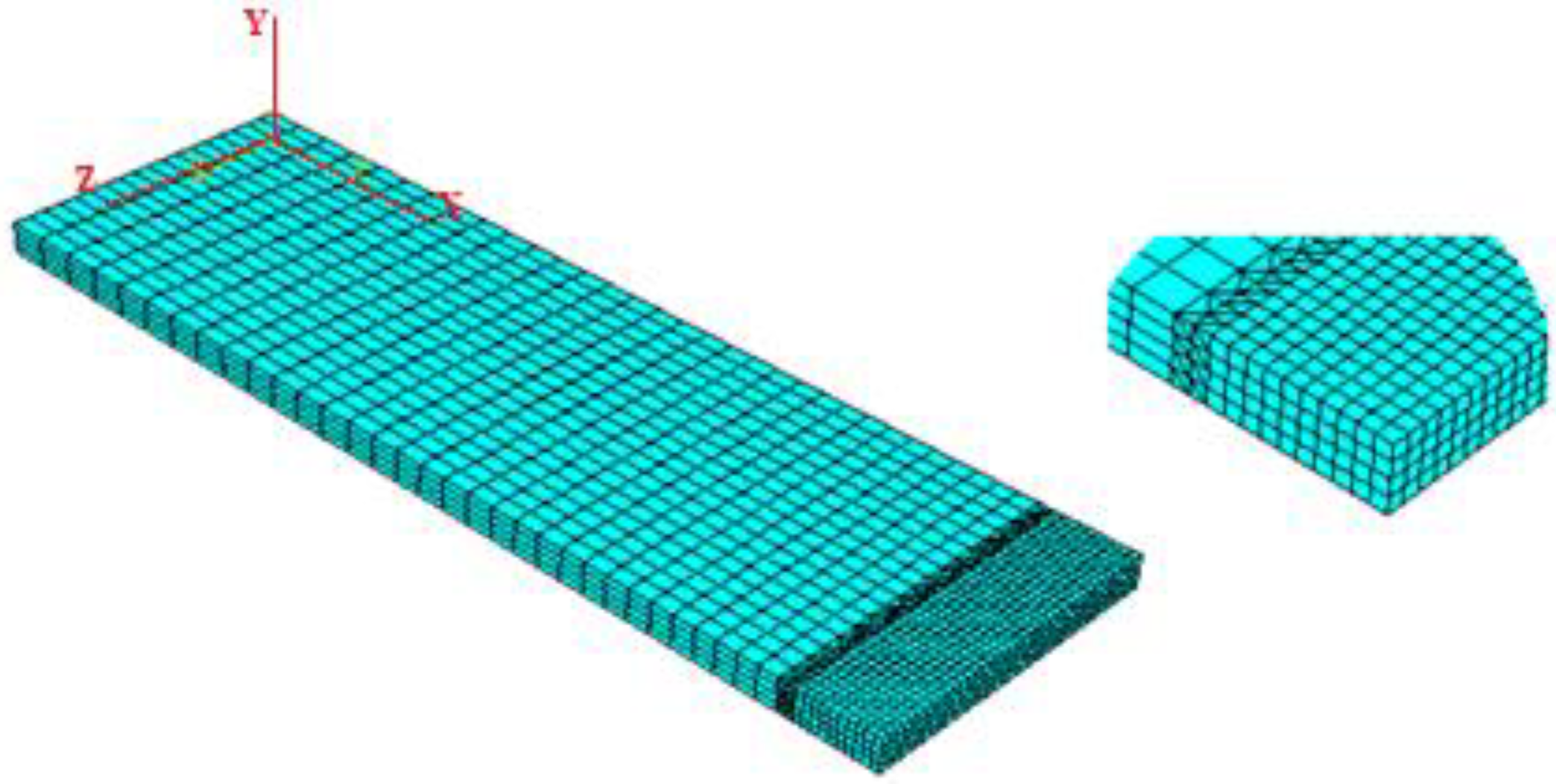
2.1.3. Meshing Technique

The accuracy and convergence of the numerical simulation results depend on the element type and the dimensions of various regions significantly. Figure 1 represents the three-dimensional geometrical model with identical mesh used in this research. Higher thermal gradient in the fusion zone and heat-affected zone and the need for more accurate temperature computation in these regions, a finer mesh is considered [16]. This subject causes us to model part geometry with two types of elements that differ in the number of nodes. The partitioning technique is utilized to separate different welding regions whose differences in experienced temperature. In thermal analysis, because of the temperature degree of freedom, DC3D8 and DC3D4 elements are used. This DC3D8 element is an eight-node linear heat transfer brick element. Therefore, it is necessary to mention that intermediate elements are utilized to connect coarser elements to more delicate elements. The DC3D4 is defined as an intermediate element. This is a four-node tetrahedron linear heat transfer element. The mesh is composed of 22,202 3D heat transfer elements. The minimum size of each element is 0.25 mm in the fusion zone (FZ).

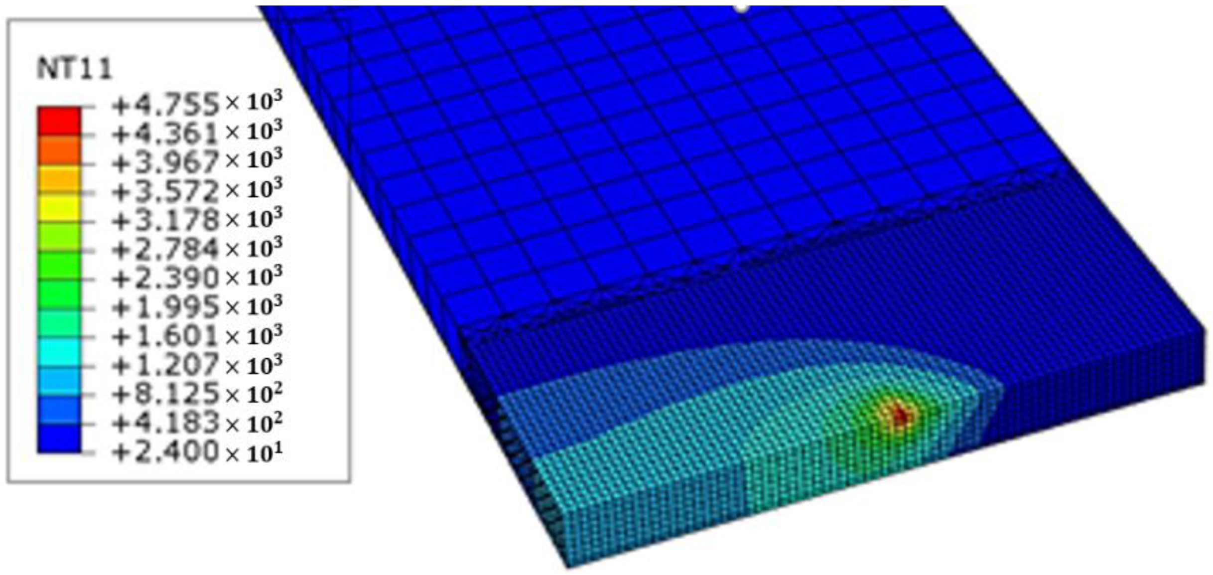
2.2. Heat Transfer Analysis

Thermal analysis during TIG welding and evaluating temperature distribution along the model is applied using the Energy conservation equation. In the transient thermal analysis of the welding process, the origin of the cartesian coordinate system is supposed to locate on the model surface; Y-axis and Z-axis are defined along the welding direction and the thickness direction, respectively. The governing equation for the 3D transient heat transfer is given by Equation (1) [18]:

$$\frac{\partial }{\partial x}\left(k_x\left(T\right)\frac{\partial T}{\partial x}\right)+\frac{\partial }{\partial y}\left(k_y\left(T\right)\frac{\partial T}{\partial y}\right)+\frac{\partial }{\partial z}\left(k_z\left(T\right)\frac{\partial T}{\partial z}\right)+Q\left(x,y,z,t\right)=p\left(T\right)c\left(T\right)\frac{\partial T}{\partial t}$$

(1)

T is the temperature, p is the material density, c is the specific heat, k is the material conductivity, and Q is the internal heat generation per unit volume. Moreover, x, y, and z are the coordinates system attached to the heat source.

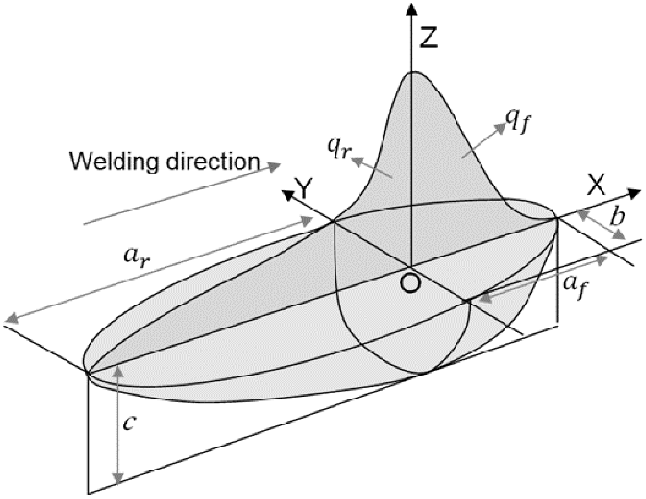
2.2.1. Heat Source Model

The accurate prediction of the fusion zone geometry and temperature distribution has a close relationship with the utilized heat source model and its parameters. In the welding process, defining the moving heat source with precise volumetric heat flux along the thickness is vital. Previous results represent that the double ellipsoid shape provides the best distribution, especially for arc welding joints; Since the double-ellipsoidal heat power density model presented by Goldak et al., is implemented in this study to simulate the TIG arc welding process [19]. Gaussian distribution of heat source is utilized to compute and analyze the thermal distribution; subsequently, dimensions of weld bead such as bead width and depth of penetration are achieved.

In the current simulation work, two rear and front ellipsoidal shapes merged, as shown in Figure 2 include two different ellipses, i.e., one in the front of the heat source and the other in the rear section.

The moving Cartesian coordinate system (x, y, and z) attached to the heat flux distribution (q) presented in Equations (2) and (3): The power density distribution inside the front quadrant is:

$$q_f=\frac{6\sqrt{3}Q{f}_f}{\pi \sqrt{\pi }{a}_{f}bc}exp\left(-3\left(\frac{x^2}{b^2}+\frac{{(y+vt)}^2}{a_f{}^2}+\frac{z^2}{c^2}\right)\right)$$

(2)

Similarly, the power density for the back of the heat source is defined as Equation (3):

$$q_r=\frac{6\sqrt{3}Q{f}_r}{\pi \sqrt{\pi }{a}_{r}bc}exp\left(-3\left(\frac{x^2}{b^2}+\frac{{(y+vt)}^2}{a_r{}^2}+\frac{z^2}{c^2}\right)\right)$$

(3)

For the front ellipse of the heat source, the front heat absorption coefficient $f_f$ defined. Also, for the rear ellipse of the heat source, the rear heat absorption coefficient $f_r$ is defined. Elliptic lengths of the front and rear sections of the heat source are different. $a_f$ is defined as front elliptical length and, $a_r$ defined as rear elliptical length. The values of parameters a, b, c in the front and rear ellipse can differ [16]. The variables of the double ellipsoidal heat source equation used in the FEM are listed in

Table 2. Double ellipsoidal heat source parameters.

Variables	Double Ellipsoidal Distribution			Heat Input Fractions
values	$a_f\left(\mathrm{mm}\right)$	$a_r\left(\mathrm{mm}\right)$	b (mm)	c (mm)	$f_f\left(\mathrm{mm}\right)$	$f_r\left(\mathrm{mm}\right)$
	5	15	10	2	0.5	1.5

. V is the scanning speed along the welding direction, and t is the current time. According to Equation (4), Q is the heat source of the TIG welding process and is equal to the multiple arc voltage (V), welding current (I), and process efficiency (η).

$$Q=\eta \times V\times I$$

(4)

To apply a moving volumetric heat source, the DFLUX user subroutine was programmed and utilized. Non-uniform distributed heat flux as a function of time and position was determined using DFLUX as an interface during thermal analysis.

2.2.2. Boundary Conditions

During thermal analysis simulation of TIG arc welding, the boundary conditions were identified for the model. The initial temperature of the model is considered 25 ℃. Heat loss through radiation and convection is considered boundary conditions. The top surface of the welding plate is exposed to a heat source, whereas the lateral surfaces during thermal analysis experience heat losses by convection and radiation only. The governing equation used for boundary condition given as Equation (5):

$$K\left(\frac{dT}{dy}\right)-q\left(x,z\right)+h\left(T-T_{\infty }\right)+\mathsf{\epsilon }\sigma \left(T^4-T_{\infty }^4\right)=0$$

(5)

where K is isotropic thermal conductivity, q is heat flux ($\mathrm{W}/{\mathrm{m}}^2\mathrm{K}$), h is the convective coefficient, T is the local temperature, $T_{\infty }$ is the ambient temperature, $\mathsf{\epsilon }$ is the emissivity coefficient, and σ is the Stefan–Boltzmann constant which is $5.67\times {10}^{-8}\mathrm{W}/{\mathrm{m}}^2{\mathrm{K}}^4$ for radiation [20].

The free convection coefficient of airflow is considered to be 10 $\mathrm{W}/{\mathrm{m}}^2\mathrm{K}$ for stainless steel. It is used for all surfaces not exposed to the shielding gas. The welding line, which is directly below the nozzle due to the shielding gas flow, experiences forced convection heat transfer. Subsequently, the heat transfer caused by the shielding gas flow is considered as forced convection heat transfer in the simulation. The following empirical relation Equation (6) initially suggested by Gardon and Cobonpue for air and later modified by Steen for any gas was used for a part of the top surface under the nozzle.

$$h=13R{e}^{1/2}P{r}^{1/3}{k}_{gas}/NPD$$

(6)

$$Re=\frac{V_{gas}\times D\times {\rho }_{gas}}{{\mu }_{gas}}$$

(7)

$$Pr=\frac{v_{gas}}{{\alpha }_{gas}}=\frac{{\mu }_{gas}{C}_{pgas}}{k_{gas}}$$

(8)

$k_{gas}$ thermal conductivity of shielding gas (W /m K), $NPD$ Nozzle-to-plate distance (m), $V_{gas}$ Shielding gas flow velocity (m/s), $v_{gas}$ Kinematic viscosity of shielding gas (m²/s), $D$ Nozzle diameter (m), ${\rho }_{gas}$ The density of shielding gas (kg/m³) ${\mu }_{gas}$ Dynamic viscosity (kg/m/s), ${\alpha }_{gas}$ Thermal diffusivity of shielding gas (m²/s) $C_{pgas}$ Specific heat of shielding gas (J/kgK). Re (Reynolds number) and Pr (Prandtl number) based on the properties of the shielding gas.

The effect of free and forced convection and radiation as thermal boundary conditions imported to the simulation model as an effective combined temperature-dependent constant ($h_c$) with Equation (9) using FILM user subroutine employed for surfaces during the welding process. Subroutine FILM calculates ($h_c$) for every integration point at a time step.

$$h_c=\left\{\begin{array}{c}0.0668\times T\left(W/{\mathrm{m}}^2\right)0<T_a<500\\ 0.231\times T-82.1\left(W/{\mathrm{m}}^2\right)500<T_a\end{array}\right.$$

(9)

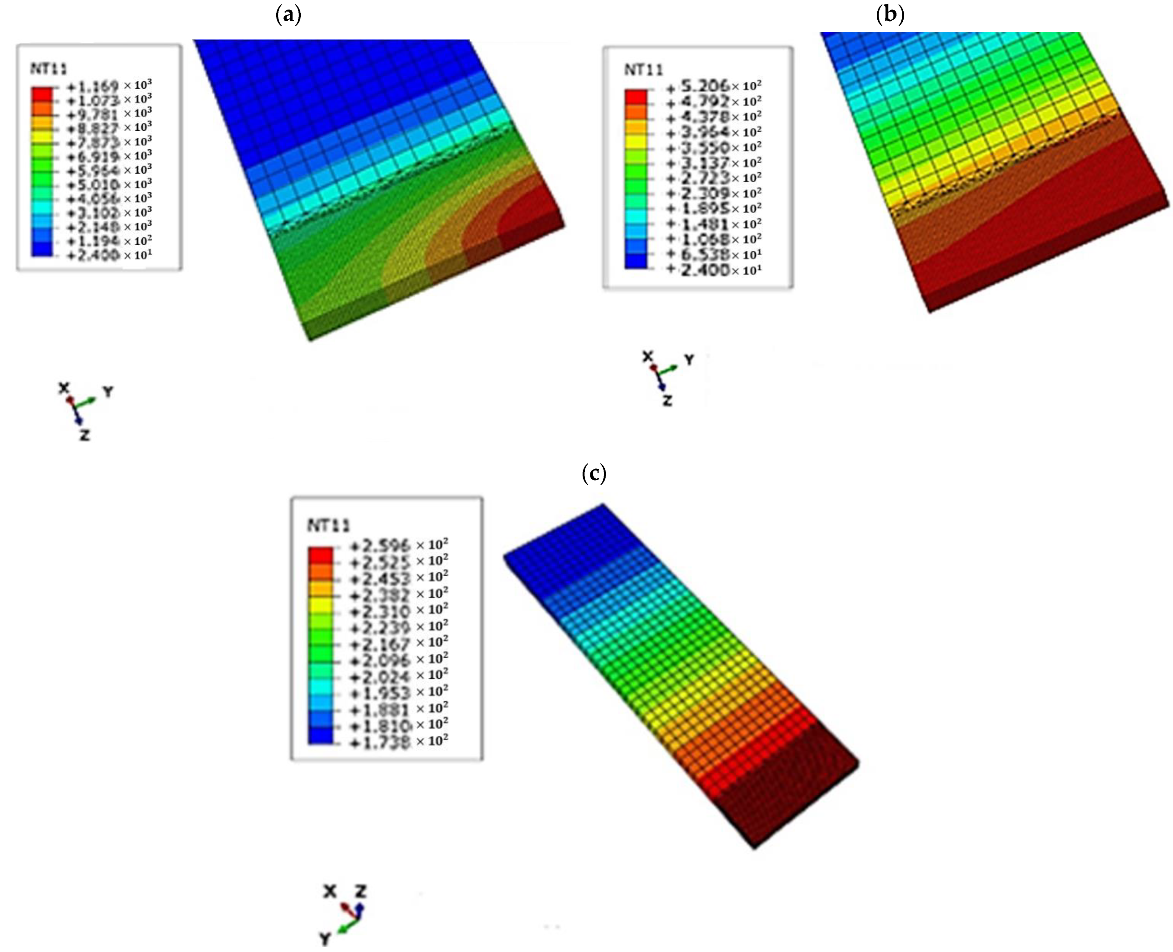
2.2.3. Post-Processing

In the current section, simulation results of the 1.4418 stainless steel TIG welding process, temperature distribution, FZ dimensions consist bead width, and depth of penetration examined. Validation of the numerical model is discussed in detail by comparing the simulation and experimental results in the results section.

3. Experimental Procedure

3.1. Welding Process

In the current study, TIG arc welding of 1.4418 stainless steel plates was carried out. Scanning speed and welding current selected as input process parameters. Also, weld bead width and depth of penetration are examined as responses. It’s worth mentioning that primarily experimentally applied a range of the input parameters simulated with FEM, and their results are analyzed. Pure argon was utilized as a shielding gas on the welding zone during the tests. The specimens were manually welded by a direct current electrode negative TIG (DCENTIG) arc with a maximum current of 250 A.

3.2. Specimen Preparation

1.4418 stainless steel was used as a material workpiece in the current work. The chemical composition is given in

Table 3. Chemical composition of 1.4418 Stainless steel.

Element	Fe	Cr	Ni	Mo	Mn	Cu	Si	W	Al	V	C
Weight percentage (%)	Bal	15.9	4.89	0.86	0.72	0.22	0.2	0.15	0.1	0.1	0.037

, which is the average of three X-ray fluorescence (XRF) measurements. The welding sheets were prepared by wire EDM with the dimensions of 127 mm × 38 mm × 4 mm. Surface grinding of the specimens was performed to eliminate the probable recast layer created by the wire EDM process [21].

3.3. Metallurgical Characterization

Welded specimens were cut by a wire-EDM process with specified dimensions transversely to examine the weld pool shape. The samples were prepared using standard metallographic techniques, which include grinding and polishing. The welding geometry responses, welding depth of penetration, and weld bead width were measured using Leica MEF 4A optical microscope (Leica Microsystems, Wetzlar, Germany) at a magnification of 50× and investigated by Clemex image software.

4. Statistical Modeling and Validation

4.1. Design of Experiments

Design of experiments (DOE) is not a series of equations, but a method utilized to organize and design tests; behind there is a theoretical basis with proper mathematical logic. Thereby, it is an essential technique for the industry and by using this method, more reliable results are obtained. Accordingly, saving more time and resources occurs. Consequently, this method assists in using a minimum number of experiments, in which several input variables varied simultaneously to reach a proper connection between them to evaluate responses. The process of modeling is generally affected by the procedure consider for designing and organizing experiments. RSM is one of these procedures, which is a series of mathematical and statistical techniques that is practical for tracking the relations between input factors and output responses [22]. When all independent variables are measurable and experiment repeated with minor errors, the RSM could be defined using Equation (10):

$$Y=f\left(x_1,x_2,x_3,\dots ,x_k\right)$$

(10)

where k is the number of independent input factors.

Finding a relationship between independent input factors and the output responses is necessary. To precise the model and responses, a quadratic polynomial is utilized generally as follows Equation (11):

$$y={\beta }_0+{\displaystyle \sum }_{i=1}^k{\beta }_i{x}_i+{\displaystyle \sum }_{i=1}^k{\mathsf{\beta }}_{ii}{x}_i^2+{\displaystyle \sum }_i{\displaystyle \sum }_j{\beta }_{ij}{x}_i{y}_j+\epsilon$$

(11)

where ${\beta }_0$ is the constant value or intercept, ${\beta }_i$ linear coefficient, ${\beta }_{ii}$ is the quadratic coefficient and ${\beta }_{ij}$ is the interaction coefficient, and ε is the random error of the developed regression. It's worth mentioning that a proposed regression model will not be a precise approximation of the actual relationship between variables in the space variable, but for a relatively limited area using such models is recommended regularly. In the current study, the experiments were organized based on a central composite design (CCD). Input factors are considered in a five-level RSM design. Welding scanning speed (V) of 1 to 5 mm/s, and welding current (C) of 80 to 120 A chosen as independent input factors. This experimental design contains ten tests: four points in the axial direction, four as factorial points in the corners of the cube, and two points in the center of the cube.

Table 4. Designed levels of TIG welding process parameters.

Variable	−2	−1	0	1	2
Welding Current (C, A)	80	90	100	110	120
Welding scanning speed (V, mm/s)	1	2	3	4	5

shows the input factors and experimental design levels demonstrated with coded and actual values.

In this study, as mentioned above, the design of experiments was carried out based on the response surface methodology using Minitab 2019 software (Minitab Inc., State College, PA, USA). Given that two levels were assigned to each of the input factors, including the welding current and welding scanning speed, ten experiments were conducted. Weld bead width and weld depth of penetration are considered as responses. The results of the experiments are presented in

Table 5. Results overview.

Tests	Input Variables (Coded Values)		Input Variables (Actual Values)		Output Responses
Sample No.	Scanning Speed (mm/s)	Current (A)	Scanning Speed (mm/s)	Current (A)	Weld Bead Width (mm)	Weld Depth of Penetration (mm)
1	−1	−1	2	90	4.35	1.17
2	+1	−1	4	90	3.54	0.97
3	−1	+1	2	110	4.85	1.53
4	+1	+1	4	110	4.51	1.41
5	−2	0	1	100	5.09	1.67
6	+2	0	5	100	3.86	1.22
7	0	−2	3	80	3.12	0.81
8	0	+2	3	120	5.98	1.84
9	0	0	3	100	4.36	1.32
10	0	0	3	100	4.19	1.08

. To obtain the mathematical models of responses and optimization, ANOVA is performed using Minitab 2019 software; F-value and adjusted R² parameters are used as criteria to fit a regression polynomial that can predict the responses minimizing the regression residuals.

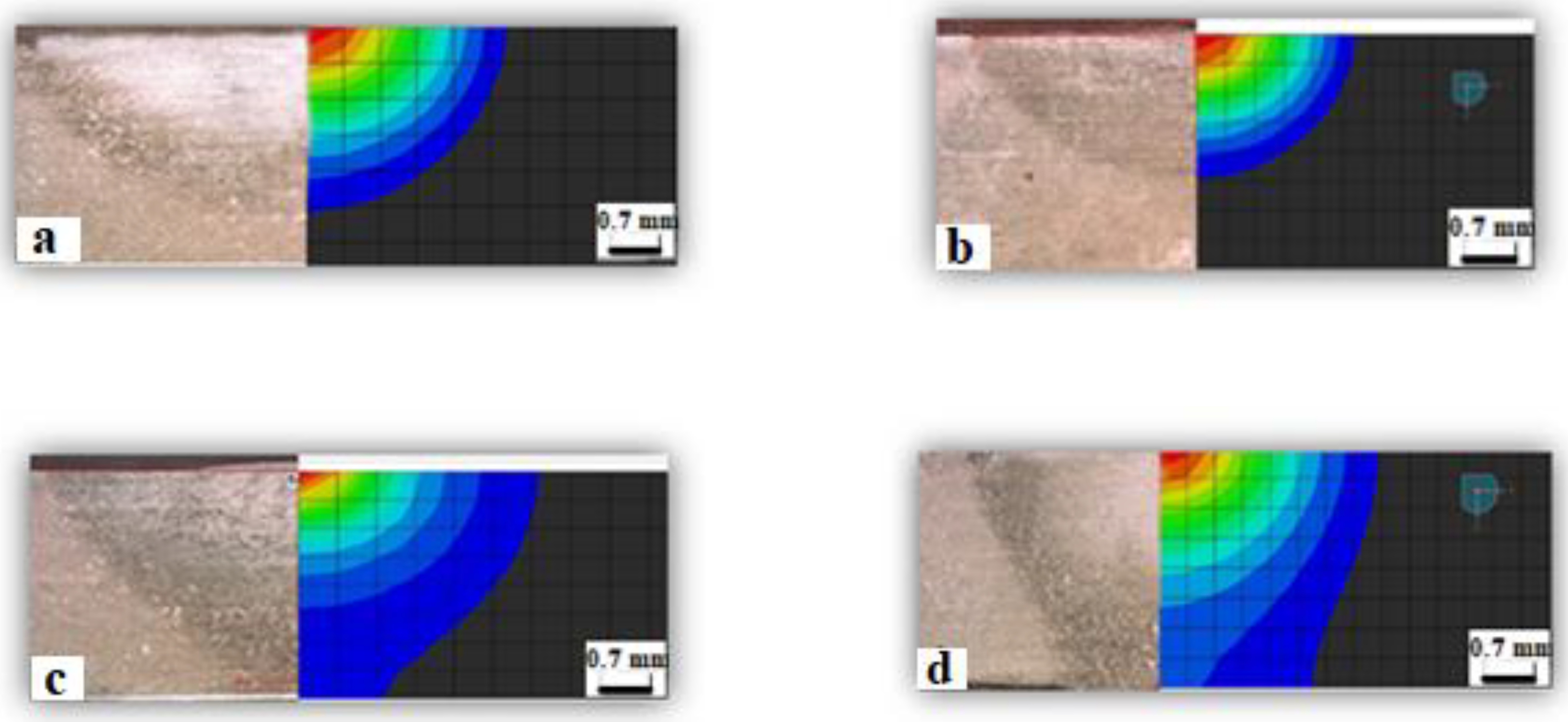
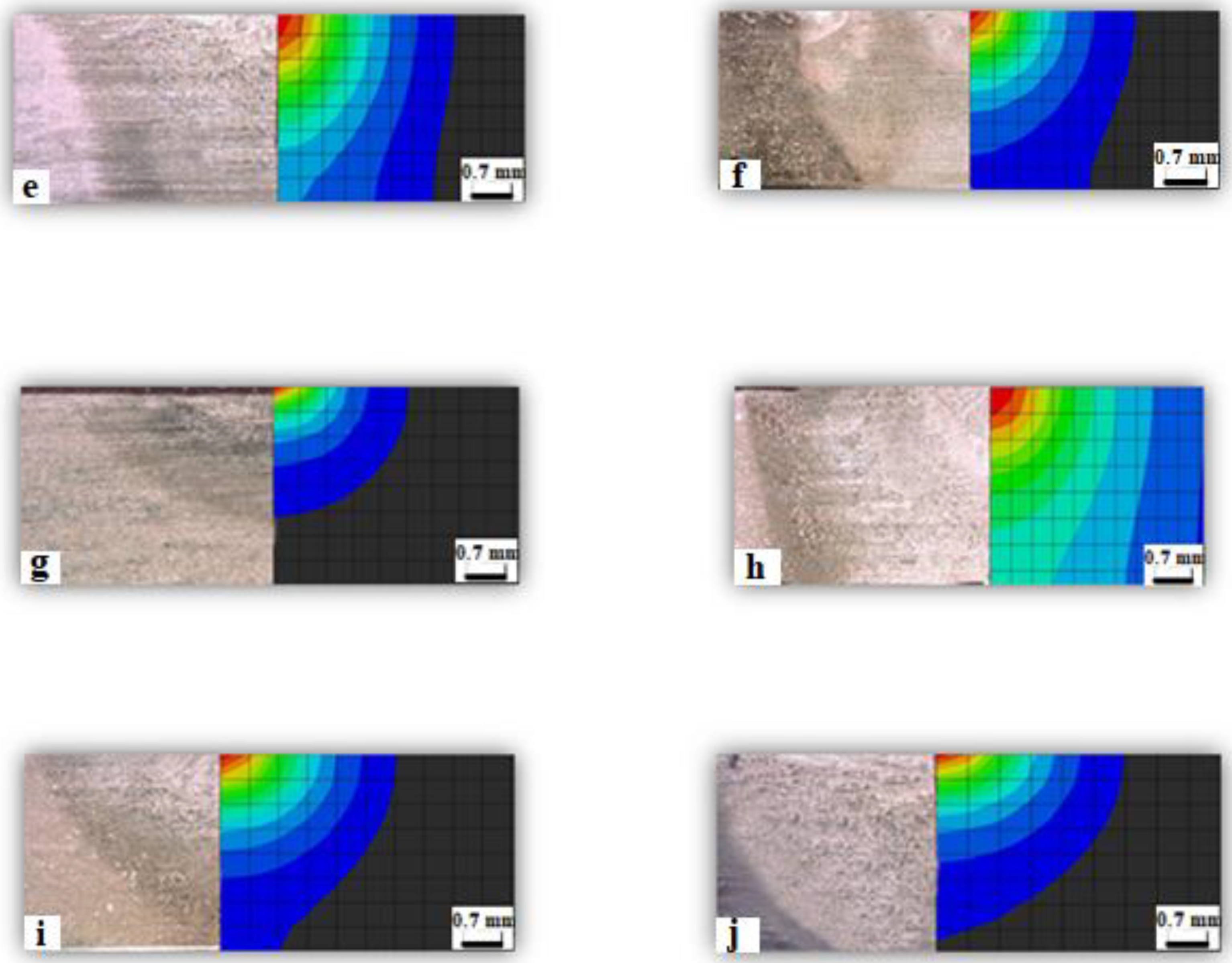
4.2. TIG Welding FEM Simulation Results

Figure 3 shows the result of thermal analysis for TIG welding of 1.4418 stainless steel. Temperature distribution with the volumetric double ellipsoidal shape at weld pool along welding line identified as a result of thermal analysis.

The predicted temperature distributions of welded parts at different increment times of the cooling time after the TIG welding process depicted in Figure 4a represents 13 s after welding; Figure 4b 50 s after welding; and Figure 4c 600 s after the welding process.

In the following, the subsequent section develops the comparative analysis for FEM simulation, and experimental approaches of weld pool dimensions include weld bead width and depth of penetration for the TIG welding process of 1.4418 stainless steel at different conditions. For the proposed purpose, primarily, three main domains FZ, HAZ, and BM, are identified as resultant regions after the TIG welding process. The Fusion zone is evaluated by all nodes whose temperatures are higher than the melting point of the 1.4418 stainless steel. It is possible to estimate the geometry and dimensions of the fusion zone from the simulation considering the applied heat flux. These distances can be measured between nodes in the simulation easily. As stated above, the experimental weld pool geometries were measured by Clemex image analysis software as well. Weld pool geometries (weld bead width and weld depth of penetration of butt welds) between FEM results and experimentally welded samples at ten different cases compared and present in

Table 6. Validation of numerical reports with experimental data.

Tests	Input Variables		Weld Bead Width			Weld Depth of Penetration
Sample No.	Scanning Speed (mm/s)	Current (A)	Experimental Results (mm)	Simulation Results (mm)	Percent Error %	Experimental Results (mm)	Simulation Results (mm)	Percent Error %
1	2	90	4.35	3.7	17	1.17	1.4	3.3
2	4	90	3.86	3.9	0.2	0.97	1	4
3	2	110	4.85	4.3	12.1	1.53	1.3	15.3
4	4	110	4.51	4.3	10.5	1.41	1.3	19.8
5	1	100	5.09	4.8	7.2	1.67	1.7	1.4
6	5	100	3.86	3.1	20	1.22	1	25.2
7	3	80	3.12	3	6	0.81	0.7	10.5
8	3	120	5.98	5.4	11.2	1.84	1.6	10.7
9	3	100	4.36	4.1	8.1	1.32	1.2	11.3
10	3	100	4.19	4.1	5.3	1.08	1.2	10.8

. Furthermore, their cross-sectional compared images were taken and depicted in Figure 5. According to reported conclusions, the average percent of relative error between experiments and predicted with the model was 9.7% placed in the permissible area. It should be said that outputs revealed a good correlation between the experimental and predicted geometries of the TIG welds at different levels; Eventually, the predicted weld pool geometries verify the proper application of the heat source model.

4.3. TIG Welding Experimental Results

In the current section, the weld bead width and weld depth of penetration are examined as process parameters. An analysis of variance (ANOVA) was conducted to investigate and specify “significantly effective parameters” on the TIG welding process and evaluate their influences on output responses. These analyses were carried out by full quadratic polynomial functions by using Minitab 2019 statistical software. Statistical data about the weld bead width and weld depth of penetration as a function of variables can be extracted and analyzed with Minitab using reported results illustrated in Table 5.

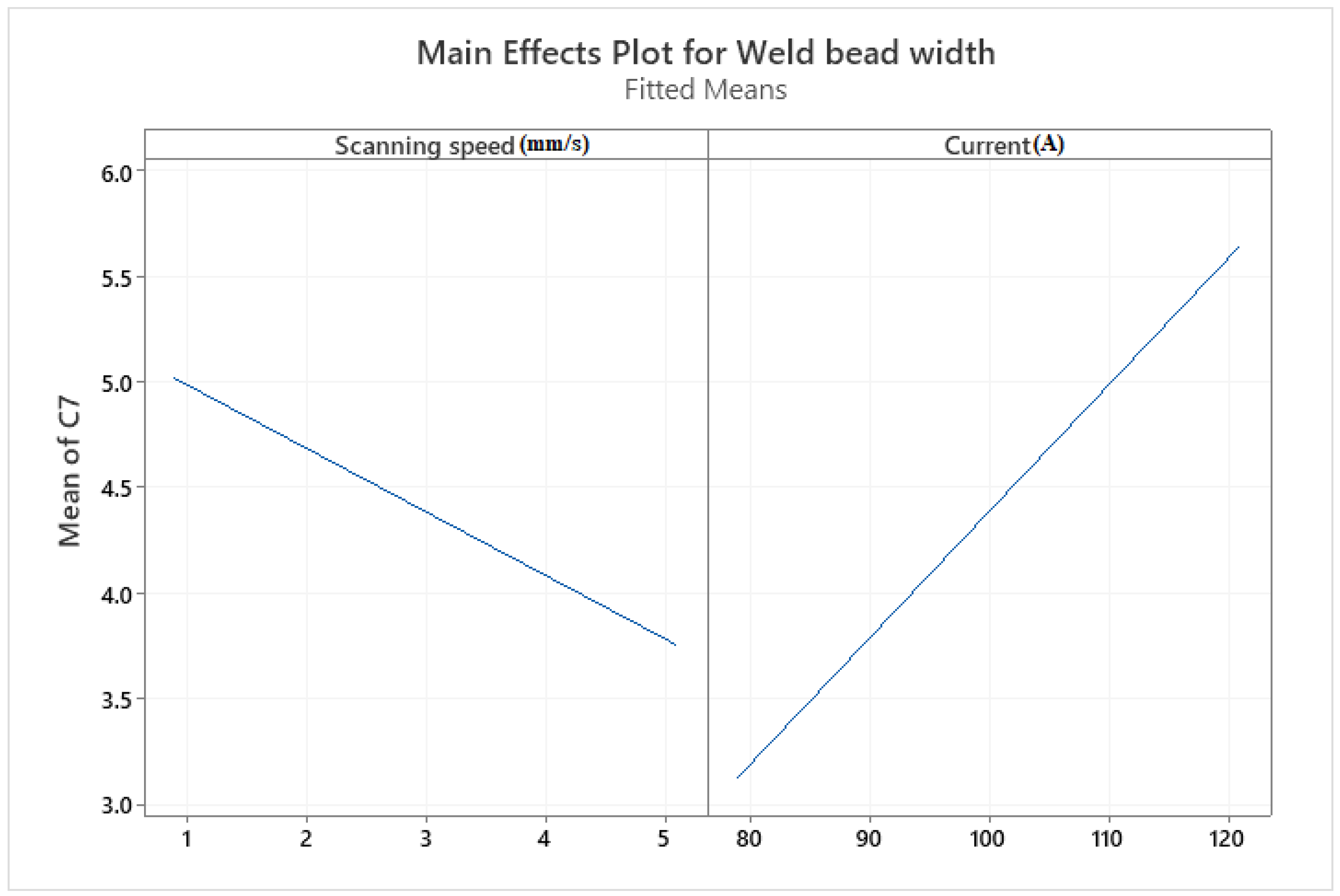
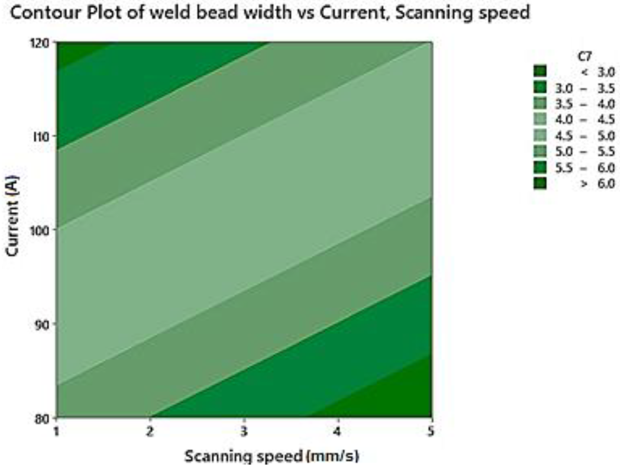
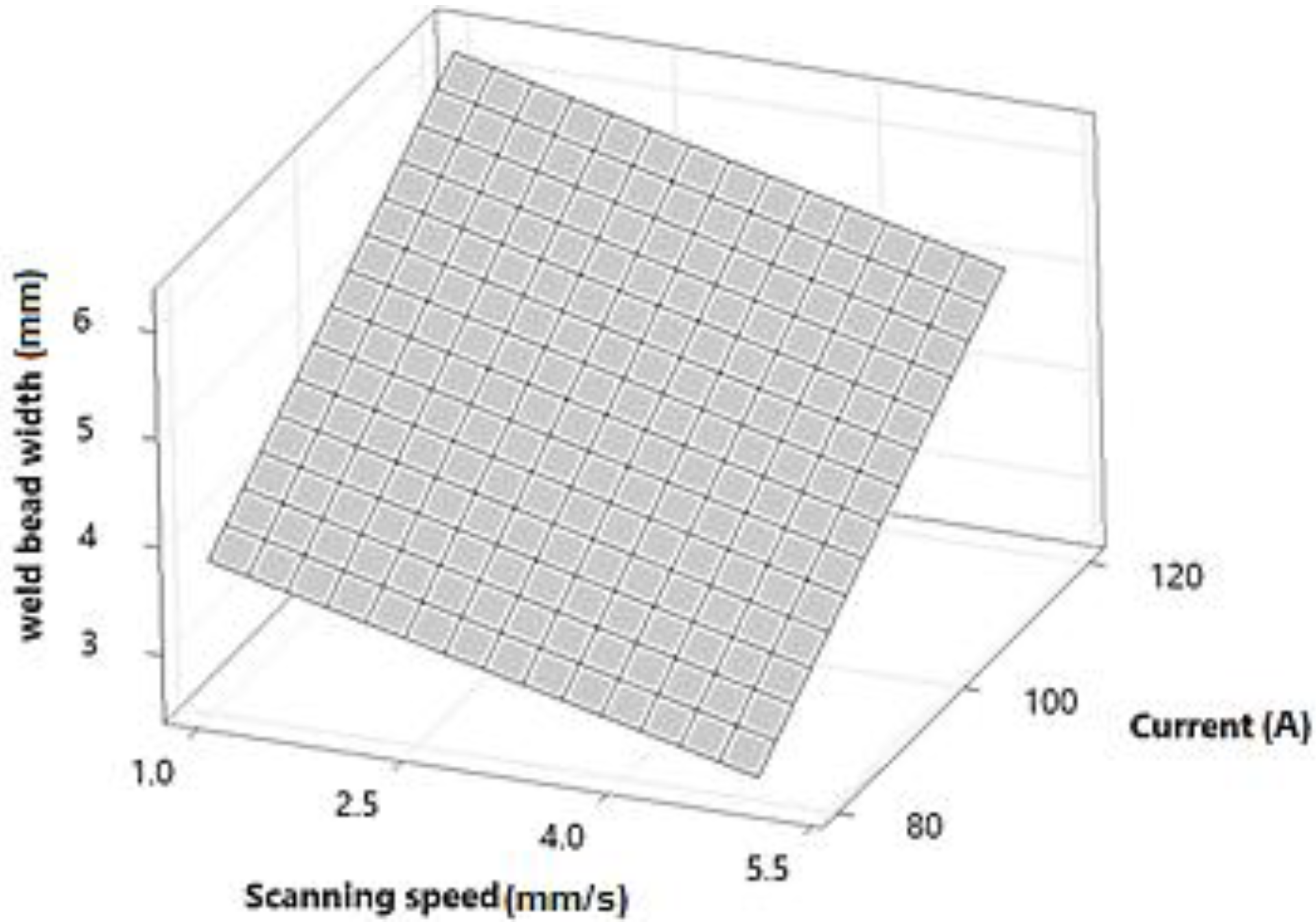
4.3.1. Weld Bead Width

According to the statistical report of an ANOVA performed on the weld bead width, all main input factors are significant, as shown in

Table 7. Revised ANOVA of the weld bead width.

Source	Sum of Squares	Degree of Freedom	Mean Square	F-Value	p-Value	VIF
Model	5.39402	2	2.69701	37.12	0.000
Scanning speed (V)	1.08601	1	1.08601	14.95	0.006	1.0
Current (C)	4.30801	1	4.30801	59.29	0.000	1.0
Lack-of-Fit	0.49418	6	0.08236	5.70	0.310
Pure Error	0.01445	1	0.01445
Total	5.90265	9
R-Squared = 91.38%			R-Squared (Adj) = 88.92%

. Among quadratic terms and interactions, none are effective. Equation (12) shows the regression model with coded values for the weld bead width considering significant parameters. The ANOVA, table of weld bead width shows that the regression model output fits the weld bead width with a good estimation. However, the lack of fit is insignificant. It should be recalled that in ANOVA if the regression model is significant whereas the lack-of-fit is insignificant simultaneously, the analysis is performed correctly.

Weld bead width (W) = −0.704 − 0.3008 × scanning speed (V) + 0.05992 × Current (C)

(12)

Figure 6 represents the main effect plots for the weld bead width response. The method used to distinguish the effect of parameters in the main effect plots is investigating the slope of the line. If the calculated line for a parameter is near horizontal; this parameter has no significant impact on response. However, a parameter with the highest inclined line will have the most significant effect. It is apparent from the plots that factor C as Current is the most influential variable. This obtained result was realized from the physical phenomenon of the TIG welding process.

Figure 7 and Figure 8 illustrate the contour and the response surface plots for weld bead width based on the input parameters. As can be seen in the contour plots, no interaction between input variables existed. There is a relation between scanning speed and current on the weld bead width, as shown in these figures. It is important to note that, the physical properties of the material extensively affect its behavior during the welding process. The 1.4418 stainless steel has low thermal conductivity among martensitic stainless steels. Low thermal conductivity causes lower heat dissipation and hence, reduces the cooling step after welding. `In this metal, FZ experiences a higher local temperature than others, due to a low heat dissipation rate. For this reason, changes in input parameters influence weld bead geometries severely. Furthermore, from a metallurgical point of view, these physical properties result in coarser grain size in the fusion zone and low hardness in this area. Therefore, with increasing current, weld bead width grows. It can be seen that overheating of metal in the fusion zone occurred with increasing the welding current at a constant scanning speed. Extending in weld bead width was due to a physical phenomenon. This is widely referred to as the Marangoni effect. Differences in surface tension cause the Marangoni effect. Fluid flow for any fluid system is always from zones with higher surface tension towards lower. The surface tension depends on the temperature as the weld center has a higher temperature compared to edges, the surface tension is lower at the edges compared to the center. Thus, fluid in the molten state was drifted from the center to the edges. It should be noted that increasing the welding current causes to rise heat input in FZ and consequently, the temperature gradient, is increased. Subsequently, the FZ and HAZ regions shorten with the reduction of the welding current.

Furthermore, reducing the scanning speed has the same effect as increasing the welding current. In such cases, different parts in the welding joints experience the same effect on the microstructure. As described above, the heat input has a direct relation with the welding current but its relationship with scanning speed is in reverse. By reducing the scanning speed, the residence time of the arc extends, and input power density—the input energy transmitted to the welding zone in the form of heat within a unit of distance—ascends, in turn, it causes to increase the melted material volume. Thus, the weld bead geometry, especially the weld bead width, is extended. Defects like undercutting occur in the weld zone when the welding current is too high [23].

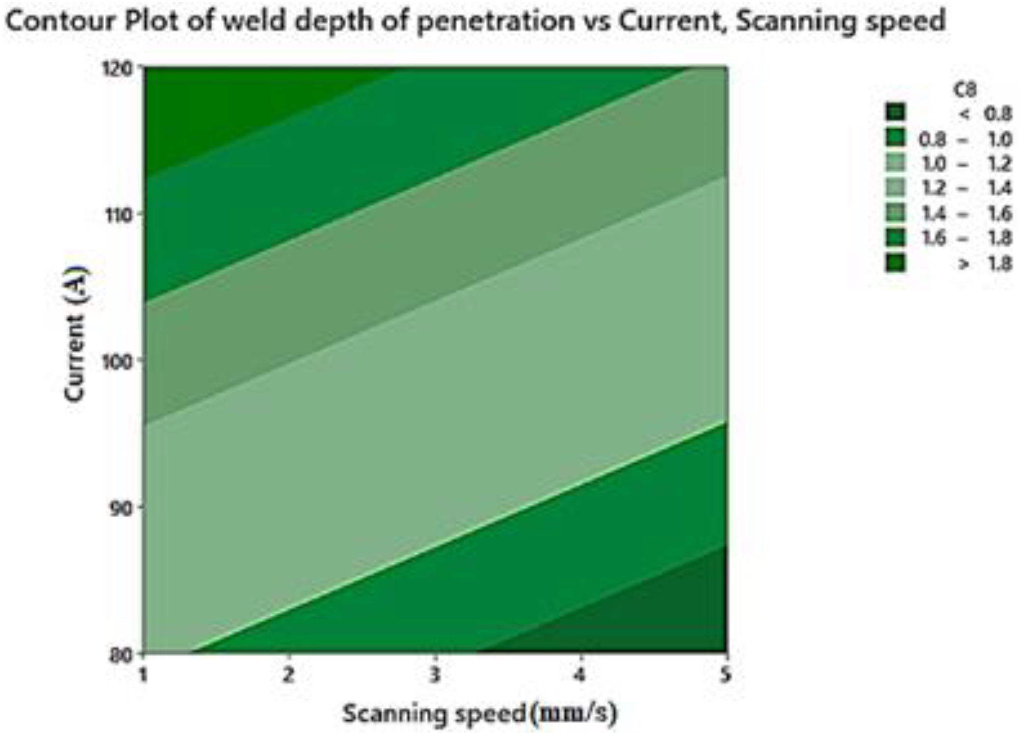
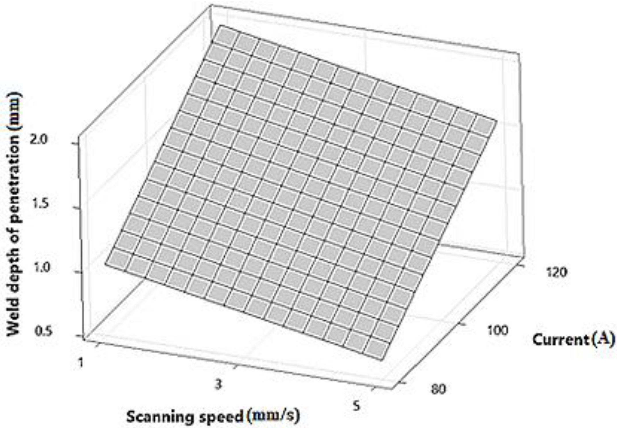
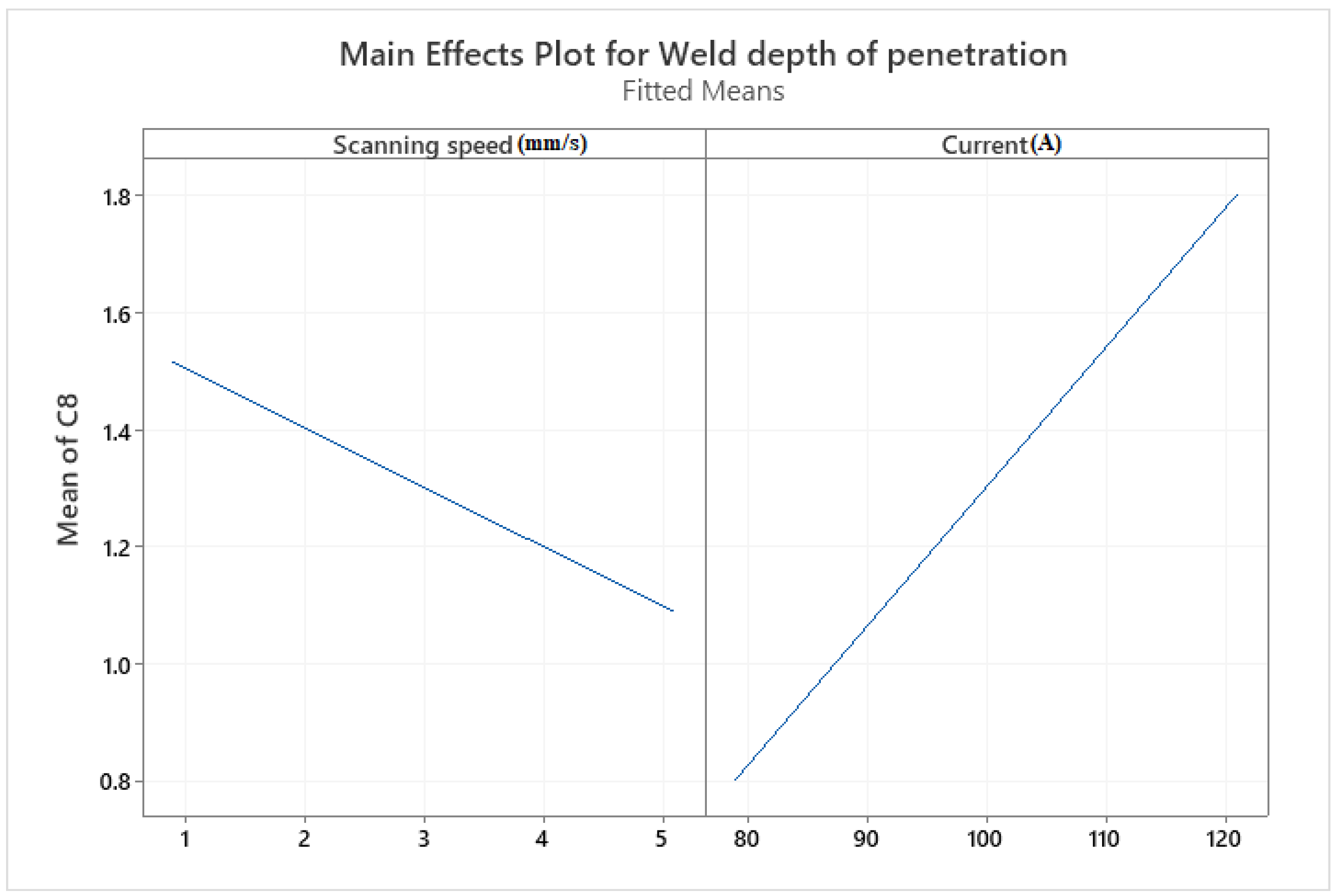
4.3.2. Weld Depth of Penetration

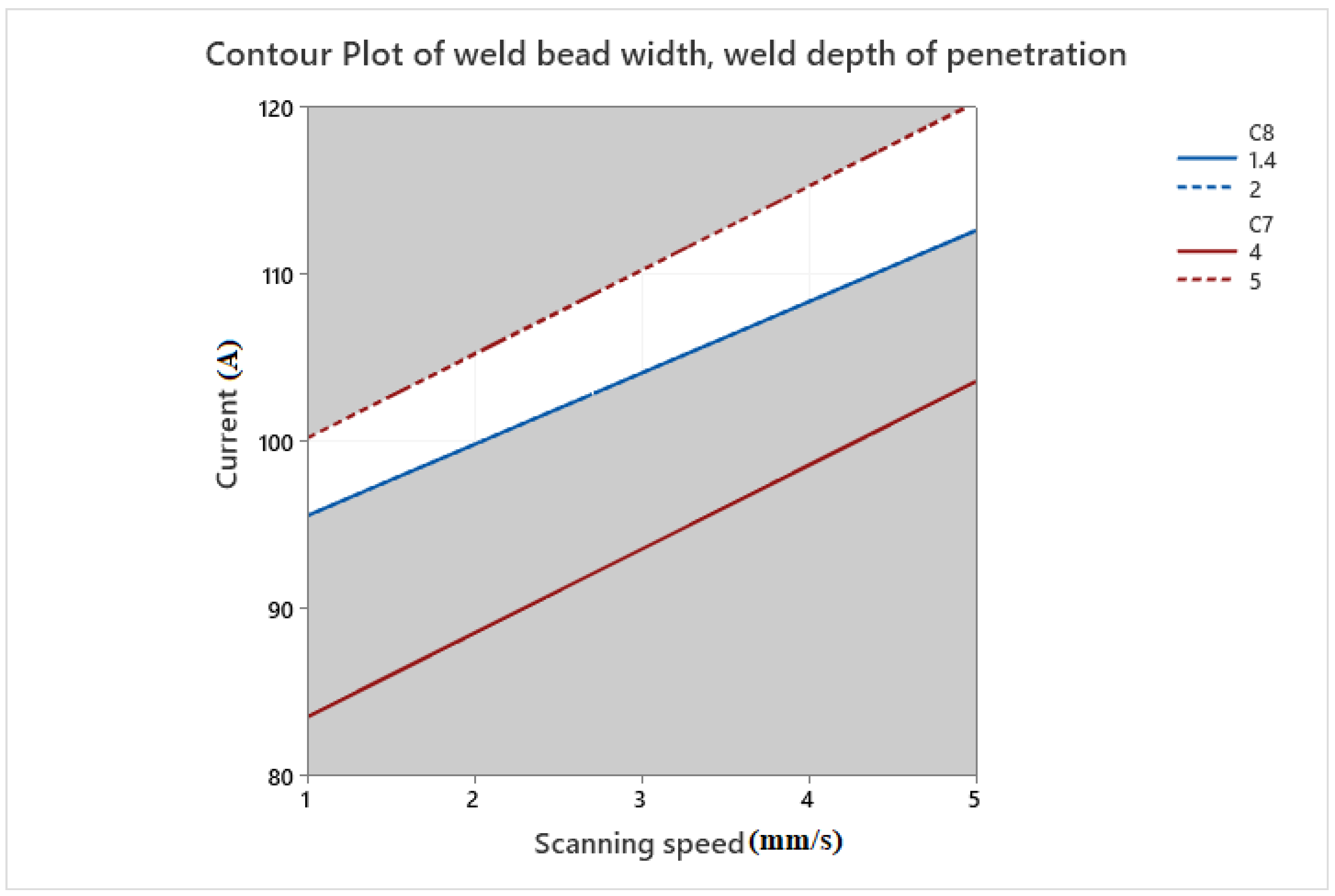
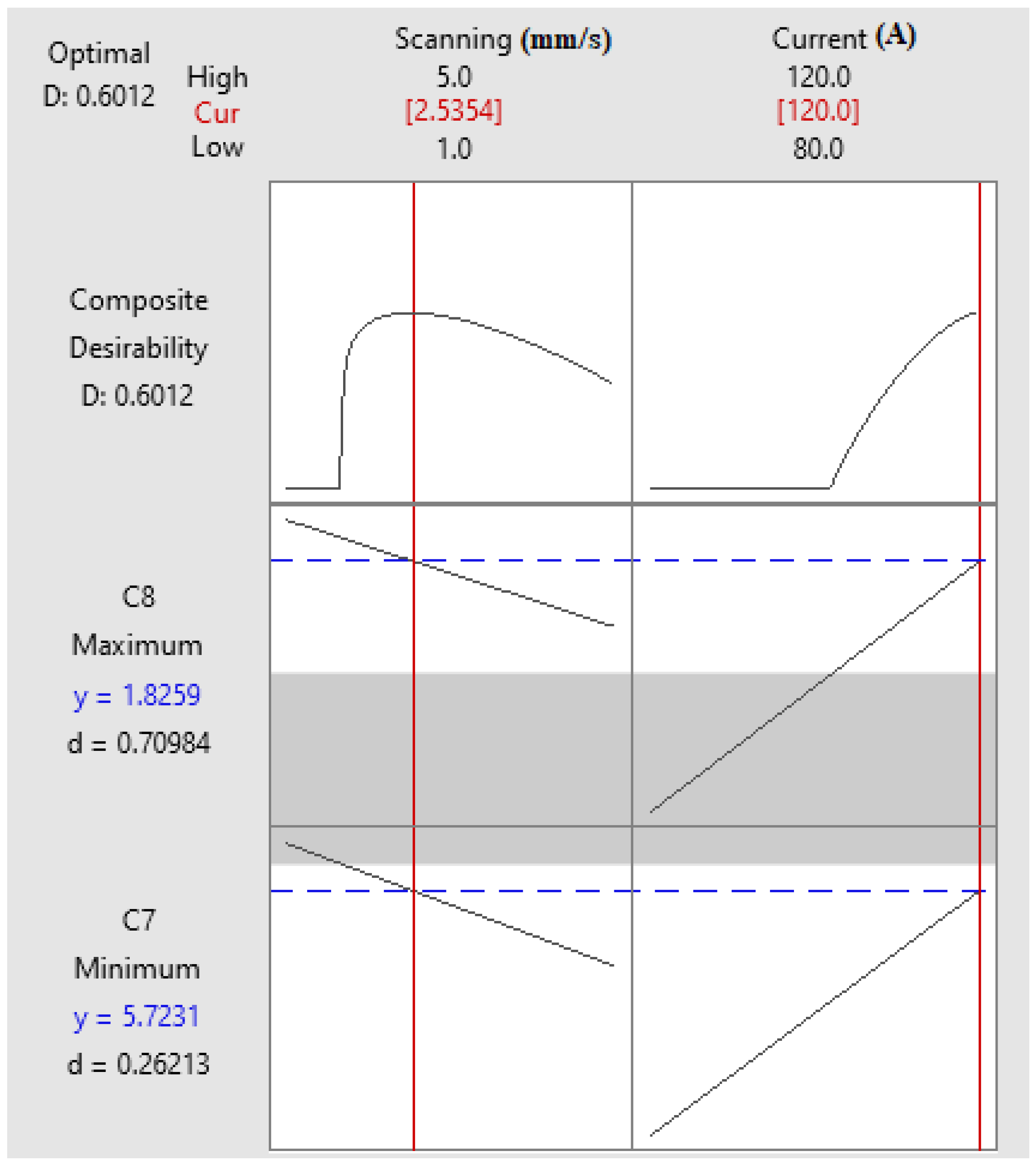
According to the statistical report of an ANOVA performed on the weld bead width, all main input factors are significant, as shown in

Table 8. Revised ANOVA of the weld depth of penetration.

Source	Sum of Squares	Degree of Freedom	Mean Square	F-Value	p-Value	VIF
Model	0.80567	2	0.40283	25.9	0.001
Scanning speed (V)	0.12403	1	0.12403	7.97	0.026	1.0
Current (C)	0.68163	1	0.68163	43.82	0.000	1.0
Lack-of-Fit	0.08009	6	0.01335	0.46	0.808
Pure Error	0.02880	1	0.02880
Total	0.91456	9
R-Squared = 88.09%			R-Squared (Adj) = 84.69%

. Among second-order terms and interactions, none are effective. Equation (13) shows the regression model with coded values for the weld bead width considering significant parameters. The ANOVA table of weld depth of penetration indicates that the regression model output fits the weld bead width with a good estimation. However, the lack of fit is insignificant. It should be recalled that in ANOVA if the regression model is significant but simultaneously the lack-of-fit is insignificant, the analysis is performed correctly.

Weld depth of penetration (P) = −0.776 − 0.1017 × Scanning speed (V) + 0.02383 × Current (C)

(13)

Figure 9 represents the main effect plots for the weld depth of penetration response. The method used to distinguish the effect of parameters in the main effect plots is investigating the slope of the line. On the one hand, the calculated line for a parameter is near horizontal; but then this parameter has no significant impact on the response. On the other hand, a parameter with the highest inclined line will have the most significant effect. It is clear from the plots that factor C as Current is the most effective variable. This obtained result could be realized from the physical phenomenon of the TIG welding process. Moreover, it should be mentioned that current and scanning speed has direct and reverse impacts on the weld depth of penetration, respectively.

Figure 10 and Figure 11 illustrate the contour and the response surface plots for weld bead width based on the input parameters. As can be seen in contour plots, no interaction between input variables existed. The relation between scanning speed and current on the weld depth of penetration is shown in these figures. With increasing current, penetration grows. We conclude that Buoyancy force is negligible in this case. The density difference of the molten metal in the weld region caused Buoyancy force. With a rise in temperature, molten metal density decreases. Due to the Buoyancy effect fluid tends to flow from high density to low density. In this case, it always tends to flow from the bottom to the surface of the weld. However, buoyancy forces are less potent as compared to other forces during TIG welding. As described above, overheating of metal in the fusion zone occurred with the increase of welding current at a constant scanning speed. It should be noted that increasing the welding current causes a rise in heat input in FZ and consequently, the temperature gradient decreases. Subsequently, the FZ and HAZ regions shorten with the reduction of the welding current. Hence, the welding current makes the FZ and HAZ regions deeper.

Furthermore, as described above, the heat input has a direct relation with the welding current but its relationship with scanning speed is in reverse. By reducing the scanning speed, the residence time of the arc extends, and input power density—the input energy transmitted to the welding zone in the form of heat within a unit of distance—ascends, in turn, it causes an increase of the melted material volume. Thus, the weld bead geometry, especially the weld depth of penetration, is shortened. Therefore, in such cases, the root of the welded joint can remain unwelded, leading to the low tensile strength and elongation of the welded joints [24].

5. Optimization

After statistical analysis of data obtained from the experimental study, the regression equations are given by Equations (5)–(7), developed for TIG welding process modeling. These equations explain logical relationships between input variables and responses. The research carried out the optimization of the TIG welding process of 1.4418 stainless steel to access optimum welding settings, which minimize weld bead width and makes full penetration.

Table 9. Optimized range of input variables and responses.

Parameter/Response		Variable	Goal	Lower	Upper	Importance	Composite Desirability
Parameters		Scanning speed	in range	1	5	---	---
		Current	in range	80	120	---	---
Response	Criteria 1	Weld bead width (W)	Minimize	3.12	5.98	1	0.57
		Weld depth of penetration (P)	Maximize	0.81	1.84	1
	Criteria 2	Weld bead width (W)	Minimize	3.12	5.98	1	0.60
		Weld depth of penetration (P)	Maximize	0.81	1.84	5
	Criteria 3	Weld bead width (W)	Minimize	3.12	5.98	1	0.53
		Weld depth of penetration (P)	Maximize	0.81	1.84	4

offers the criteria for the optimization of input factors. In Table 9, the importance values and composite desirability of all three responses are mentioned, and as one may see, weld penetration is more important than the other ones. The optimization was performed according to the criteria mentioned in Table 9. The optimum setting was achieved by using Minitab software, which is presented in

Table 10. Predicted optimum point.

Solution		Optimum Input Parameters		Composite Desirability %		Output Responses
		Scanning Speed	Current			Weld Bead Width	Weld Depth of Penetration
1	Coded value	−0.2	+2	54%	Predicted	5.67449	1.80947
	Actual value	2.69697	120

. In addition to maximizing depth penetration and minimizing weld bead width, it should be noted that the low productivity of TIG welding should be covered and optimized [25].

In criteria 1 of the optimum conditions, partial penetration occurs. Criteria 3 is chosen as the best condition of this process because of the better quality and the higher scanning speed compared to criteria 2. Optimal settings of experimental tests carried out at the optimized predicted results due to verifying statistical analysis. Table 10 depicts the predicted results of criteria 2. Figure 12 describes Derringer’s desirability with graphs.

Figure 13 illustrates an overlay plot composed of the contour plots from each response stacked on top of each other to create the combined plot. The developed white area reveals the final optimal factor settings of experimental tests. On the other hand, the undesirable area grayed out.

The over plot suggests an accepted area to achieve the desired condition for responses [26].

6. Conclusions

In this investigation, the simulation model is primarily developed for the TIG welding process on 1.4418 stainless steel sheets followed by a mathematical model with Abaqus and validated with experimental approaches. In the following, the effect of the scanning speed and the current are investigated in this process by using Minitab software. According to numerical, experimental, and statistical works, the following results concluded:

• Among the input variables of 1.4418 stainless steel TIG welding, scanning speed is the most significant factor with a reverse effect on all weld bead dimensions.
• Results revealed that increasing the current and decreasing scanning speed, causes the weld bead width to widen and the depth of penetration extended, due to increased input energy transmitted to the material and it conducts to an increase in the melted volume.
• By applying a multi-objective optimization, through the desirability approach, the optimum settings of the TIG welding process are scanning speed (V) = 2.69 mm/s, Current (C) = 120 A.
• In the highest desired condition, the weld bead width of the welded part diminishes to 5.7 mm, and the depth of penetration increases to 1.8 mm.
• By conducting the thermal FEM analysis tests for 10 different cases and comparing them with experimental approaches, the predicted model has an average 9.7% relative error. As a result, this model shows the robustness of the present FEM model utilized for TIG Arc welding of 1.4418 stainless steel.
• With obtained results in this research, we can choose optimum input factors to reach a convenient weld seam with full penetration weld and wide weld bead. Moreover, with these input factors, optimum samples with high mechanical strength can be reached.

Although the results of this study are promising, the research can be extended to analyze the presented method on a wide range of materials. Future studies can also include mechanical analyses such as residual stress and surface deformation of the weld pool. Finally, microstructural analyses of the welding area can be considered to describe the heat-affected zone (HAZ).

References

1. Kumar, A.; Dixit, P.K. Investigating the effects of filler material and heat treatment on hardness and impact strength of TIG weld. Mater. Today Proc. 2019, 26, 2776–2782. [Google Scholar] [CrossRef]
2. Ramakrishnan, A.; Rameshkumar, T.; Rajamurugan, G.; Sundarraju, G.; Selvamuthukumaran, D. Experimental investigation on mechanical properties of TIG welded dissimilar AISI 304 and AISI 316 stainless steel using 308 filler rod. Mater. Today Proc. 2021, 45, 8207–8211. [Google Scholar] [CrossRef]
3. Singh, S.R.; Khanna, P. A-TIG (activated flux tungsten inert gas) welding: A review. Mater. Today Proc. 2020, 44, 808–820. [Google Scholar] [CrossRef]
4. Kadir, M.H.A.; Asmelash, M.; Azhari, A. Investigation on welding distortion in stainless steel sheet using gas tungsten arc welding process. Mater. Today Proc. 2020, 46, 1674–1679. [Google Scholar] [CrossRef]
5. Xia, C.; Pan, Z.; Fei, Z.; Zhang, S.; Li, H. Vision based defects detection for Keyhole TIG welding using deep learning with visual explanation. J. Manuf. Process. 2020, 56, 845–855. [Google Scholar] [CrossRef]
6. Kumar, P.; Kumar, R.; Arif, A.; Veerababu, M. Investigation of numerical modelling of TIG welding of austenitic stainless steel (304L). Mater. Today Proc. 2020, 27, 1636–1640. [Google Scholar] [CrossRef]
7. Vinoth, V.; Sudalaimani, R.; Veera Ajay, C.; Suresh Kumar, C.; Sanjeevi Prakash, K. Optimization of mechanical behaviour of TIG welded 316 stainless steel using Taguchi based grey relational analysis method. Mater. Today Proc. 2021, 45, 7986–7993. [Google Scholar] [CrossRef]
8. Kumar, M.S.; Begum, S.R. Simulation of hybrid (LASER-TIG) welding of stainless steel plates using design of experiments. Mater. Today Proc. 2020, 37, 3755–3758. [Google Scholar] [CrossRef]
9. Wang, Q.; Sun, D.L.; Na, Y.; Zhou, Y.; Han, X.L.; Wang, J. Effects of TIG welding parameters on morphology and mechanical properties of welded joint of Ni-base superalloy. Procedia Eng. 2011, 10, 37–41. [Google Scholar] [CrossRef] [Green Version]
10. Natrayan, L.; Anand, R.; Kumar, S.S. Optimization of process parameters in TIG welding of AISI 4140 stainless steel using Taguchi technique. Mater. Today Proc. 2020, 37, 1550–1553. [Google Scholar] [CrossRef]
11. Narang, H.; Singh, U.; Mahapatra, M.; Jha, P. Prediction of the weld pool geometry of TIG arc welding by using fuzzy logic controller. Int. J. Eng. Sci. Technol. 2012, 3, 77–85. [Google Scholar] [CrossRef] [Green Version]
12. Reda, R.; Magdy, M.; Rady, M. Ti–6Al–4V TIG Weld Analysis Using FEM Simulation and Experimental Characterization. Iran. J. Sci. Technol.-Trans. Mech. Eng. 2020, 44, 765–782. [Google Scholar] [CrossRef]
13. Sridhara, S.N.S.; Allada, S.C.S.; Sai, P.V.S.; Banala, S.; Subbiah, R.; Marichamy, S. Tensile strength performance and optimization of Al 7068 using TIG welding process. Mater. Today Proc. 2020, 45, 2017–2021. [Google Scholar] [CrossRef]
14. Panji, M.; Baskoro, A.S.; Widyianto, A. Effect of Welding Current and Welding Speed on Weld Geometry and Distortion in TIG Welding of A36 Mild Steel Pipe with V-Groove Joint. IOP Conf. Ser. Mater. Sci. Eng. 2019, 694, 012026. [Google Scholar] [CrossRef]
15. Venkata Krishna, D.; Mahesh, E.; Kiran, G.; Suchethan, G.S.; Mouli, G.C. Numerical Analysis on the effect of welding parameters in TIG welding for INCONEL 625 alloy. Int. J. Eng. Tech. 2016, 2, 134–140. [Google Scholar]
16. Aghaee Attar, M.; Ghoreishi, M.; Malekshahi Beiranvand, Z. Prediction of weld geometry, temperature contour and strain distribution in disk laser welding of dissimilar joining between copper & 304 stainless steel. Optik (Stuttg). 2020, 219, 165288. [Google Scholar] [CrossRef]
17. Moradi, M.; Ghoreishi, M.; Rahmani, A. Numerical and Experimental Study of Geometrical Dimensions on Laser-TIG Hybrid Welding of Stainless Steel 1.4418. J. Mod. Process. Manuf. Prod. 2016, 5, 21–31. [Google Scholar]
18. Baruah, M.; Bag, S. Influence of pulsation in thermo-mechanical analysis on laser micro-welding of Ti6Al4V alloy. Opt. Laser Technol. 2017, 90, 40–51. [Google Scholar] [CrossRef]
19. Goldak, J.; Chakravarti, A.; Bibby, M. A new finite element model for welding heat sources. Metall. Trans. B. 1984, 15, 299–305. [Google Scholar] [CrossRef]
20. Casalino, G.; Michele, D.; Perulli, P. FEM model for TIG hybrid laser butt welding of 6 mm thick austenitic to martensitic stainless steels. Procedia CIRP. 2020, 88, 116–121. [Google Scholar] [CrossRef]
21. Moradi, M.; Ghoreishi, M.; Torkamany, M.J. Modelling and optimization of Nd:YAG laser and tungsten inert gas (TIG) hybrid welding of stainless steel. Lasers Eng. 2014, 27, 211–230. [Google Scholar]
22. Moradi, M.; Moghadam, M.K.; Shamsborhan, M.; Beiranvand, Z.M.; Rasouli, A.; Vahdati, M.; Bakhtiari, A.; Bodaghi, M. Simulation, statistical modeling, and optimization of CO2 laser cutting process of polycarbonate sheets. Optik (Stuttg). 2021, 225, 164932. [Google Scholar] [CrossRef]
23. Moradi, M.; Ghoreishi, M.; Khorram, A. Process and Outcome Comparison Between Laser, Tungsten Inert Gas (TIG) and Laser-TIG Hybrid Welding. Lasers Eng. 2018, 39, 379–391. [Google Scholar]
24. Zhang, B.; Shi, Y.; Cui, Y.; Wang, Z.; Hong, X. Prediction of keyhole TIG weld penetration based on high-dynamic range imaging. J. Manuf. Process. 2021, 63, 179–190. [Google Scholar] [CrossRef]
25. Aminzadeh, A.; Parvizi, A.; Moradi, M. Multi-objective topology optimization of deep drawing dissimilar tailor laser welded blanks; experimental and finite element investigation. Opt. Laser Technol. 2020, 125, 106029. [Google Scholar] [CrossRef]
26. Tahmasbi, V.; Ghoreishi, M.; Zolfaghari, M. Investigation, sensitivity analysis, and multi-objective optimization of effective parameters on temperature and force in robotic drilling cortical bone. Proc. Inst. Mech. Eng. Part. H J. Eng. Med. 2017, 231, 1012–1024. [Google Scholar] [CrossRef]
Figure 1. A Simulation model with different mesh sections.
Metals 11 01659 g001
Figure 2. Goldak’s double ellipsoidal heat source model [16].
Metals 11 01659 g002
Figure 3. TIG welding thermal analysis (NT11 reveals temperature values in ℃).
Metals 11 01659 g003
Figure 4. Different cooling times after welding consist (a) 13 s after welding (b) 50 s after welding (c) 600 s after welding.
Metals 11 01659 g004
Figure 5. Cross-sectional microscopic images from numerical and experimental approaches. (a) case: V: 2 mm/s,C: 90A; (b) case: V: 4 mm/s, C: 90A; (c) case: V: 2 mm/s,C:110A; (d) case: V: 4 mm/s, C: 110A; (e) case: V: 1 mm/s, C: 100A; (f) case: V: 5 mm/s, C: 100A; (g) case: V: 3 mm/s, C: 80A; (h) case: V: 3 mm/s, C: 120A; (i) case: V: 3 mm/s, C: 100A; (j) case: V: 3 mm/s, C: 100A.
Metals 11 01659 g005aMetals 11 01659 g005b
Figure 6. Main effects plot for weld bead width.
Metals 11 01659 g006
Figure 7. Contour plot of weld bead width.
Metals 11 01659 g007
Figure 8. Surface plot of weld bead width.
Metals 11 01659 g008
Figure 9. Main effects plot for weld depth of penetration.
Metals 11 01659 g009
Figure 10. Contour plot of weld depth penetration.
Metals 11 01659 g010
Figure 11. Surface plot of weld depth of penetration.
Metals 11 01659 g011
Figure 12. Derringer’s desirability graph.
Metals 11 01659 g012
Figure 13. Overlay contour plot.
Metals 11 01659 g013