Modeling of the Evolution of the Microstructure and the Hardness Penetration Depth for a Hypoeutectoid Steel Processed by Grind-Hardening

Abstract
1. Introduction
2. Materials and Methods
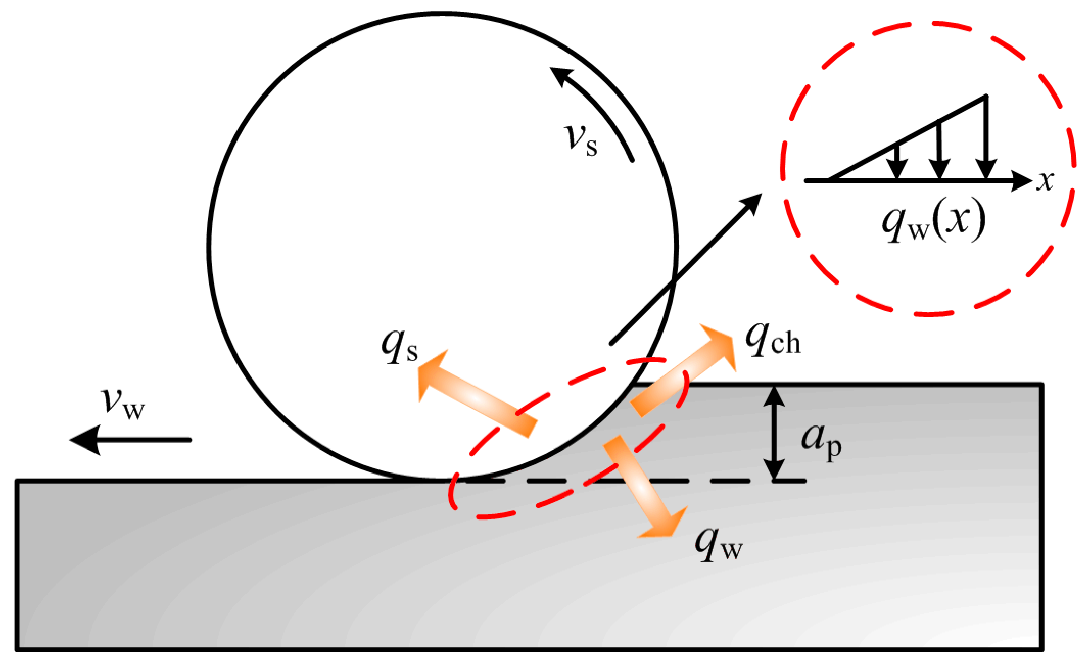
2.1. Heat Source Model for Grind-Hardening Process
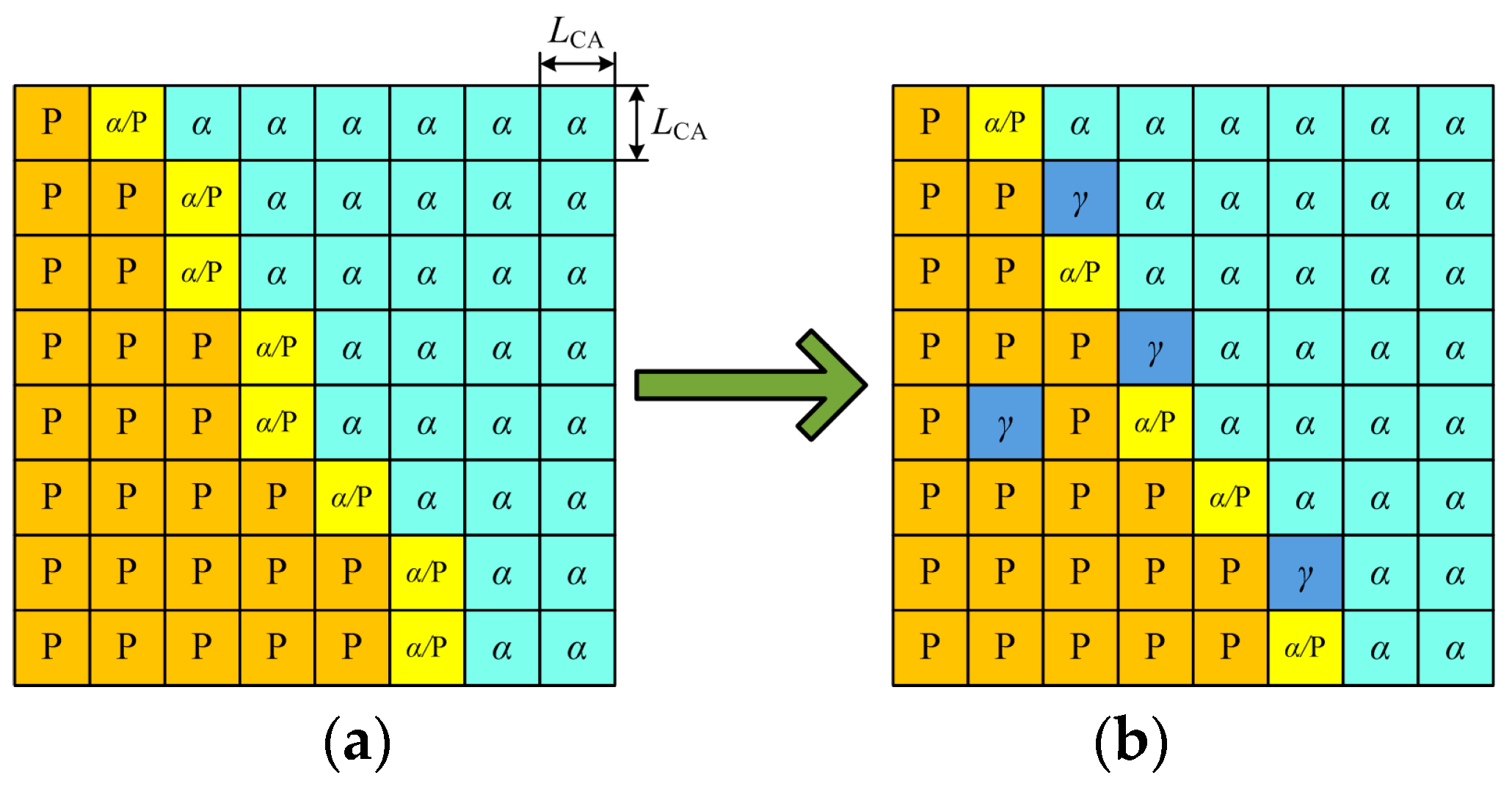
2.2. Dynamic Model for Microstructure Transformation Based on CA
2.2.1. Determination of Austenitization Starting Temperature
2.2.2. Dynamic Model for Austenite Transformation
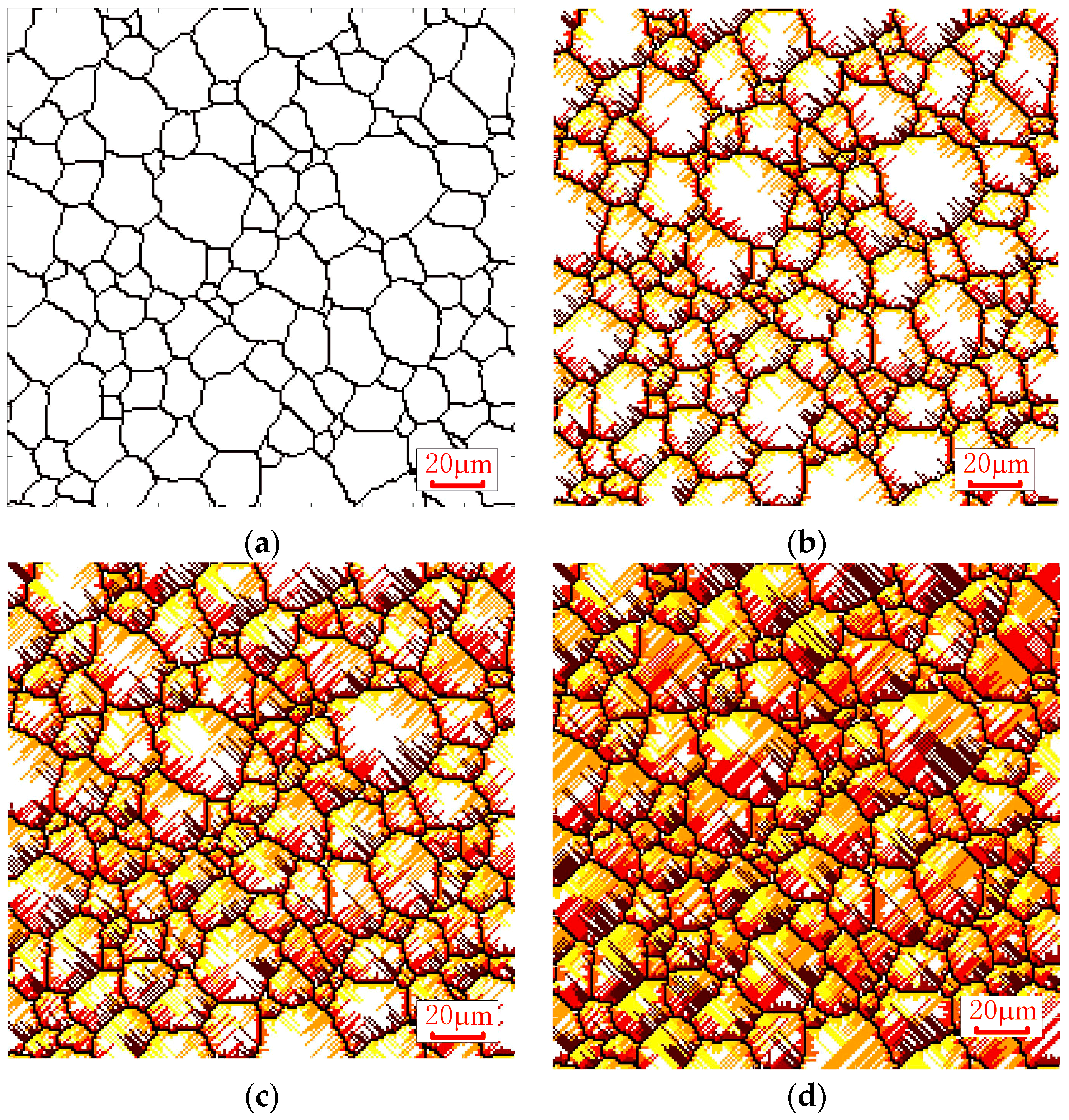
2.2.3. Dynamics Model of Martensitic Transformation
3. Results and Discussions
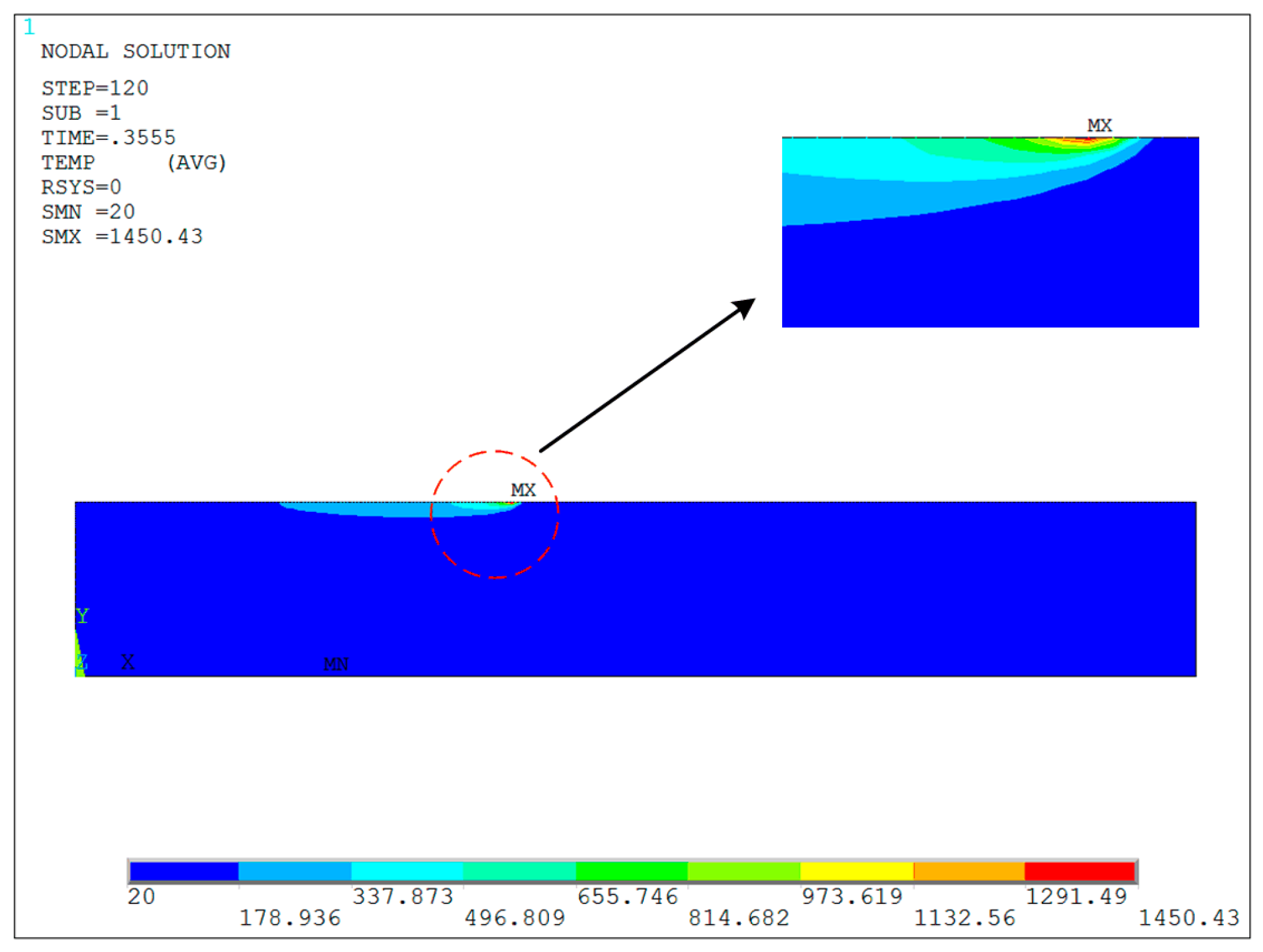
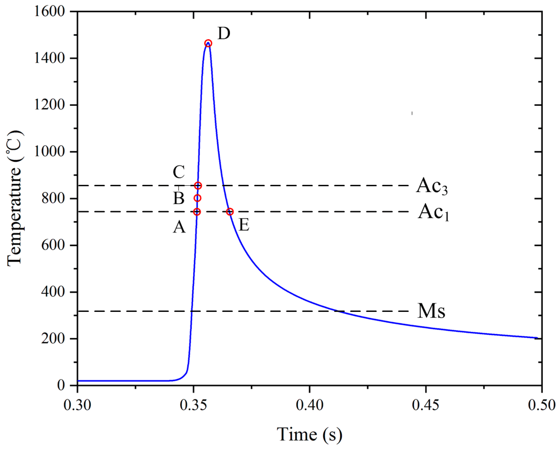
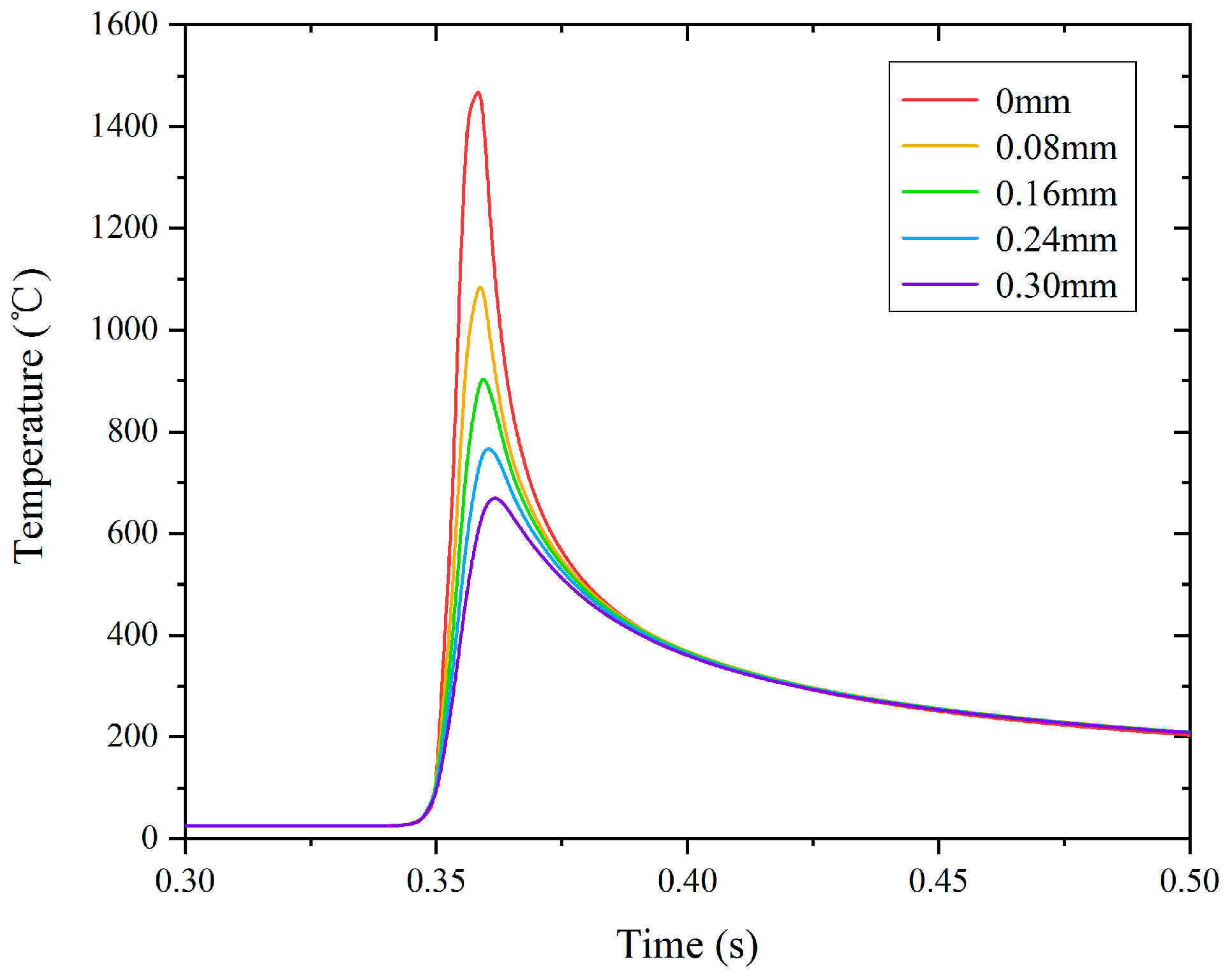
3.1. Temperature Field Simulation and Discussion of Hardened Layer
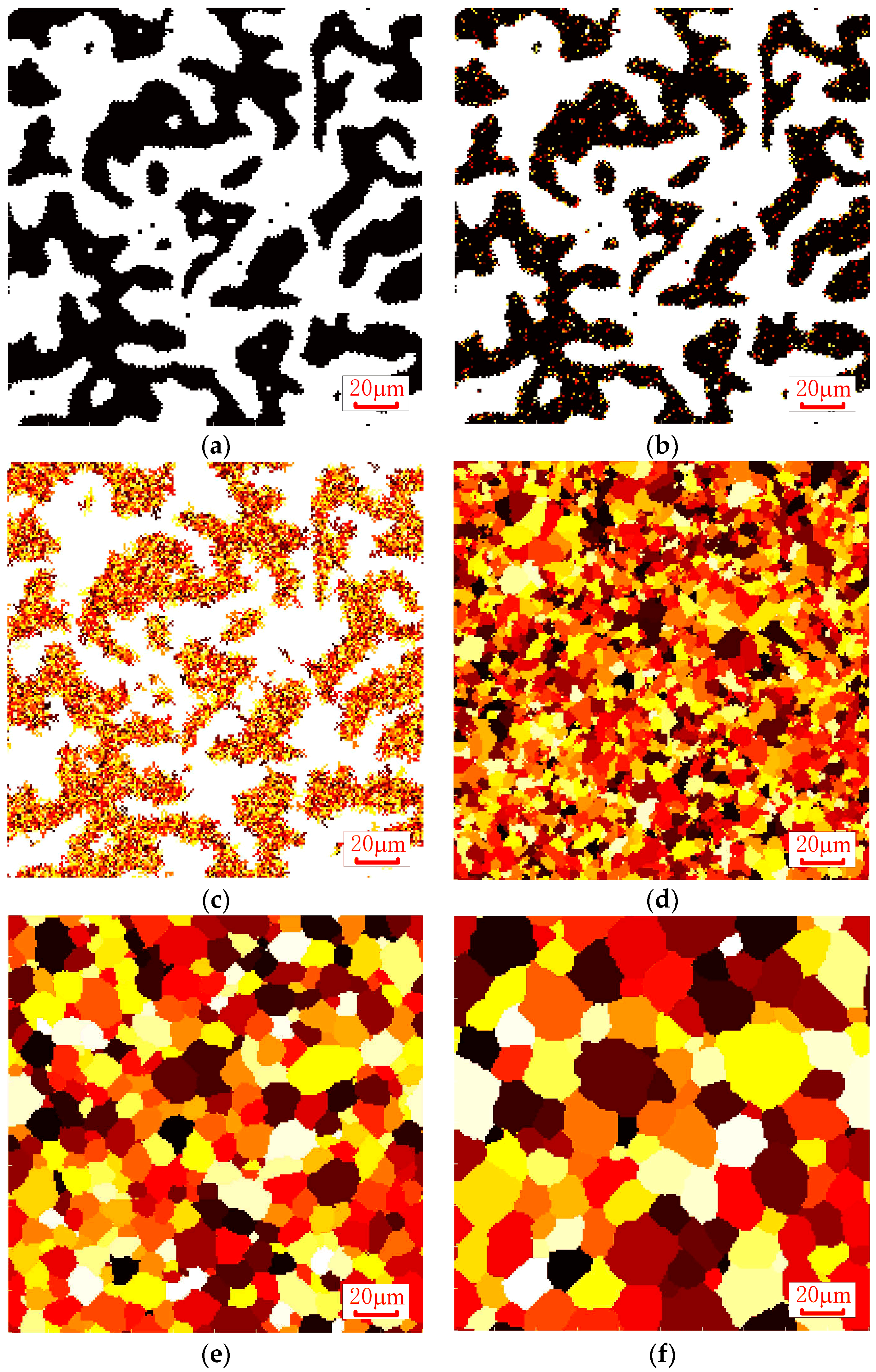
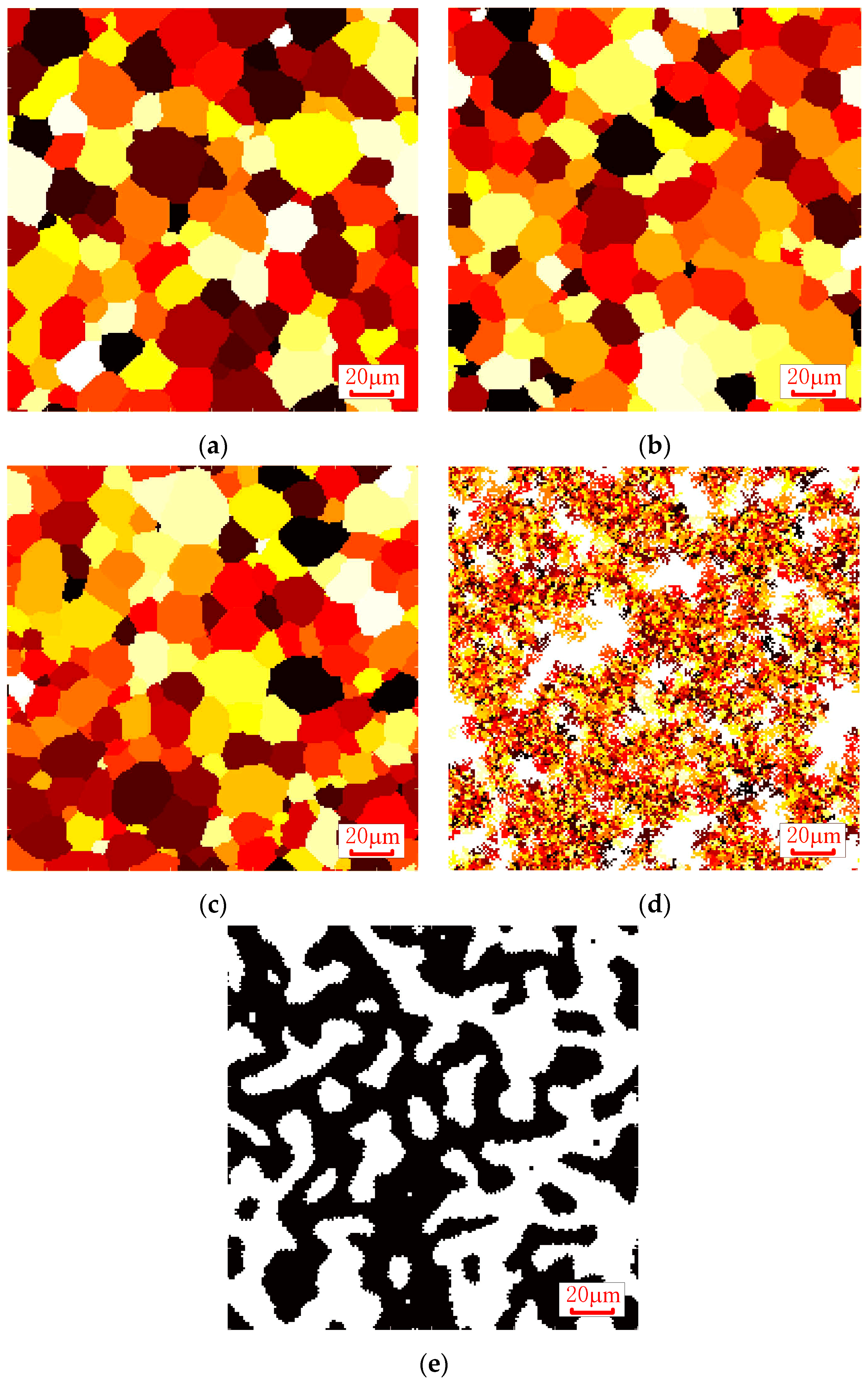
3.2. Microstructure Transformation Simulation of Hardened Layer
3.2.1. CA Model
3.2.2. Microstructure Transformation Simulation of Hardened Layer
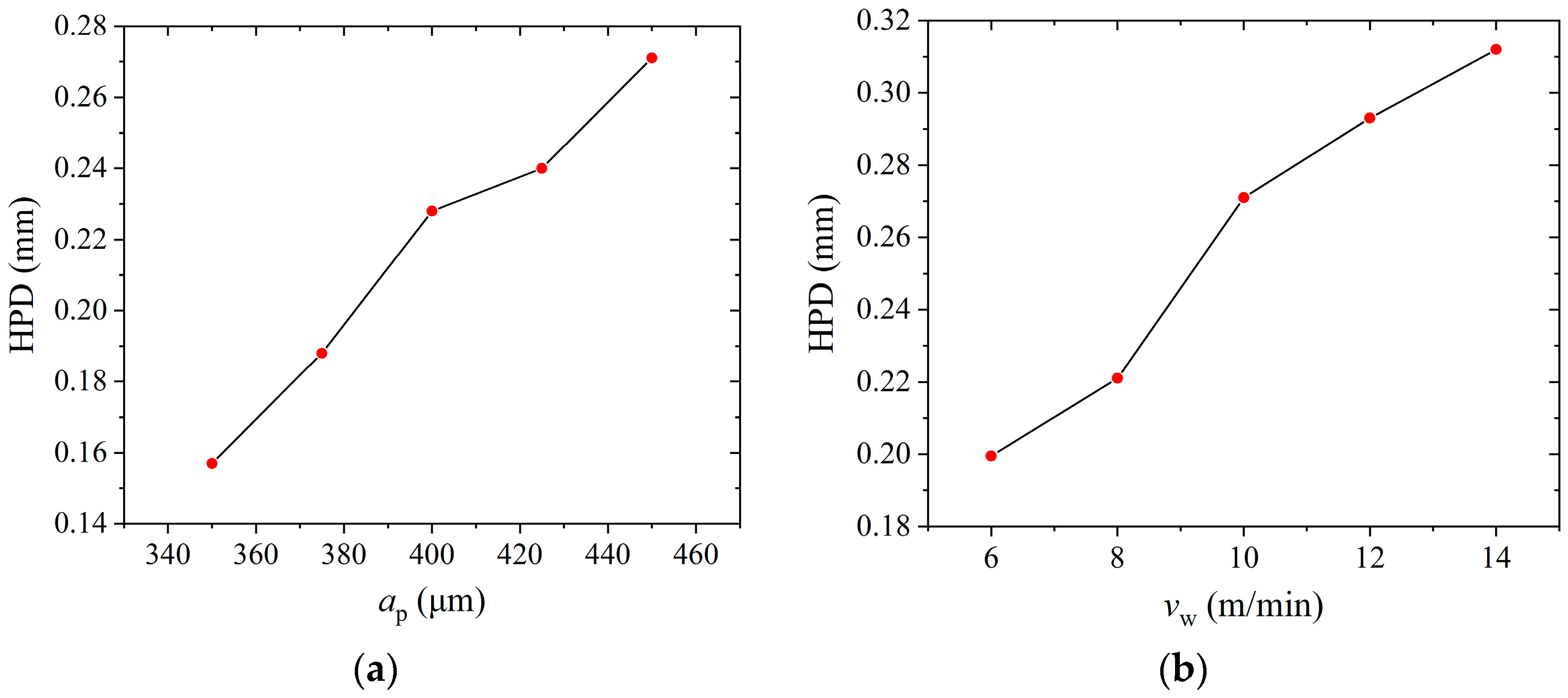
3.2.3. Prediction of HPD
4. Experimental Validation of the Analysis
5. Conclusions
Author Contributions
Funding
Acknowledgments
Conflicts of Interest
References
- Brinksmeier, E.; Brockhoff, T. Utilization of grinding heat as a new heat treatment process. CIRP Ann. Manuf. Technol. 1996, 45, 283–286. [Google Scholar] [CrossRef]
- Deng, Y.S.; Xiu, S.C.; Shi, X.L.; Sun, C.; Wang, Y.S. Study on the effect mechanisms of pre-stress on residual stress and surface roughness in PSHG. Int. J. Adv. Manuf. Technol. 2017, 88, 3243–3256. [Google Scholar] [CrossRef]
- Nguyen, T.; Zhang, L.C.; Sun, D.L.; Wu, Q. Characterizing the mechanical properties of the hardened layer induced by grinding-hardening. Mach. Sci. Technol. 2014, 18, 277–298. [Google Scholar] [CrossRef]
- Brinksmeier, E.; Brockhoff, T. Surface heat treatment by using advanced grinding processes. Metall. Ital. 1999, 91, 19–23. [Google Scholar]
- Brockhoff, T. Grind-hardening: A comprehensive view. CIRP Ann. Manuf. Technol. 1999, 48, 255–260. [Google Scholar] [CrossRef]
- Foeckerer, T.; Zaeh, M.F.; Zhang, O.B. A three-dimensional analytical model to predict the thermo-metallurgical effects within the surface layer during grinding and grind-hardening. Int. J. Heat Mass Transf. 2013, 56, 223–237. [Google Scholar] [CrossRef]
- Alonso, U.; Ortega, N.; Sanchez, J.A.; Pombo, I.; Izquierdo, B.; Plaza, S. Hardness control of grind-hardening and finishing grinding by means of area-based specific energy. Int. J. Mach. Tools Manuf. 2015, 88, 24–33. [Google Scholar] [CrossRef]
- Liu, S.Y.; Yang, G.; Zheng, J.Q.; Liu, X.H. Numerical and experimental studies on grind-hardening cylindrical surface. Int. J. Adv. Manuf. Technol. 2015, 76, 487–499. [Google Scholar] [CrossRef]
- Huang, X.M.; Ren, Y.H.; Wu, W.; Li, T. Research on grind-hardening layer and residual stresses based on variable grinding forces. Int. J. Adv. Manuf. Technol. 2019, 103, 1045–1055. [Google Scholar] [CrossRef]
- Zhao, Y.; Chen, D.F.; Long, M.J.; Arif, T.T.; Qin, R.S. A Three-Dimensional Cellular Automata Model for Dendrite Growth with Various Crystallographic Orientations During Solidification. Metall. Mater. Trans. B 2014, 45, 719–725. [Google Scholar] [CrossRef]
- Sieradzki, L.; Made, L. A perceptive comparison of the cellular automata and Monte Carlo techniques in application to static recrystallization modeling in polycrystalline materials. Comput. Mater. Sci. 2013, 67, 156–173. [Google Scholar] [CrossRef]
- Salehi, M.S.; Serajzadeh, S. Simulation of static recrystallization in non-isothermal annealing using a coupled cellular automata and finite element model. Comput. Mater. Sci. 2012, 53, 145–152. [Google Scholar] [CrossRef]
- Monshat, H.; Serajzadeh, S. Simulation of austenite decomposition in continuous cooling conditions: A cellular automata-finite element modeling. Ironmak. Steelmak. 2019, 46, 513–521. [Google Scholar] [CrossRef]
- Yang, B.J.; Chuzhoy, L.; Johson, M.L. Modeling of reaustenitization of hypoeutectoid steels with cellular automaton method. Comput. Mater. Sci. 2007, 41, 186–194. [Google Scholar] [CrossRef]
- An, D.; Pan, S.Y.; Hang, L.; Dai, T.; Krakauer, B.; Zhu, M.F. Modeling of Ferrite-Austenite Phase Transformation Using a Cellular Automaton Model. ISIJ Int. 2014, 54, 422–429. [Google Scholar] [CrossRef]
- Halder, C.; Bachniak, D.; Madej, L.; Chakraborti, N.; Pietrzyk, M. Sensitivity Analysis of the Finite Difference 2-D Cellular Automata Model for Phase Transformation during Heating. ISIJ Int. 2015, 55, 285–292. [Google Scholar] [CrossRef]
- Su, F.Y.; Liu, W.L.; Wen, Z. Three-dimensional cellular automaton simulation of austenite grain growth of Fe-1C-1.5Cr alloy steel. J. Mater. Res. Technol. 2020, 9, 180–187. [Google Scholar] [CrossRef]
- Yu, X.X.; Lau, W.S. A finite-element analysis of residual stress in stretch grinding. J. Mater. Process Technol. 1999, 94, 13–22. [Google Scholar] [CrossRef]
- Guo, Y.; Xiu, S.C.; Liu, M.H.; Shi, X.L. Uniformity mechanism investigation of hardness penetration depth during grind-hardening process. Int. J. Adv. Manuf. Technol. 2017, 89, 2001–2010. [Google Scholar] [CrossRef]
- Yang, B.J.; Hattiangadi, A.; Li, W.Z.; Zhou, G.F.; McGreevy, T.E. Simulation of steel microstructure evolution during induction heating. Mater. Sci. Eng. A 2010, 527, 2978–2984. [Google Scholar] [CrossRef]
- Sun, C.; Duan, J.C.; Lan, D.X.; Liu, Z.X.; Xiu, S.C. Prediction about ground hardening layers distribution on grinding chatter by contact stiffness. Arch. Civ. Mech. Eng. 2018, 18, 1626–1642. [Google Scholar] [CrossRef]
- Zhu, B.; Zhang, Y.S.; Wang, C.; Liu, P.X.; Liang, W.K.; Li, J. Modeling of the Austenitization of Ultra-high Strength Steel with Cellular Automation Method. Metall. Mater. Trans. A 2014, 45A, 3161–3171. [Google Scholar] [CrossRef]
- Su, B.; Han, Z.Q.; Liu, B.C. Cellular Automaton Modeling of Austenite Nucleation and Growth in Hypoeutectoid Steel during Heating Process. ISIJ Int. 2013, 53, 527–534. [Google Scholar] [CrossRef]
- Halder, C.; Madej, L.; Pietrzyk, M. Discrete micro-scale cellular automata model for modeling phase transformation during heating of dual phase steels. Arch. Civ. Mech. Eng. 2014, 14, 96–103. [Google Scholar] [CrossRef]
- Sun, C.; Liu, Z.X.; Lan, D.X.; Duan, J.C.; Xiu, S.C. Study on the influence of the grinding chatter on the workpiece’s microstructure transformation. Int. J. Adv. Manuf. Technol. 2018, 96, 3861–3879. [Google Scholar] [CrossRef]
- Zheng, C.W.; Xiao, N.M.; Li, D.Z.; Li, Y.Y. Microstructure prediction of the austenite recrystallization during multi-pass steel strip hot rolling: A cellular automaton modeling. Comput. Mater. Sci. 2008, 44, 507–514. [Google Scholar] [CrossRef]
- Andrews, K.W. Empirical formulae for calculation of some transformation temperatures. J. Iron Steel Inst. 1965, 203, 721–727. [Google Scholar]
- Liu, M.H.; Zhang, K.; Xiu, S.C. Mechanism investigation of hardening layer hardness uniformity based on grind-hardening process. Int. J. Adv. Manuf. Technol. 2017, 88, 3185–3194. [Google Scholar] [CrossRef]
- Deng, Y.S.; Xiu, S.C. Research on microstructure evolution of austenitization in grinding hardening by cellular automata simulation and experiment. Int. Adv. Manuf. Technol. 2017, 93, 2599–2612. [Google Scholar] [CrossRef]
- Zhi, Y.; Liu, W.J.; Liu, X.H. Simulation of Martensitic Transformation of High Strength and Elongation Steel by Cellular Automaton. Adv. Mat. Res. 2014, 1004–1005, 235–238. [Google Scholar] [CrossRef]


| Temperature/°C | 20 | 100 | 200 | 300 | 400 | 500 | 600 | 700 | 800 | 900 | 1000 |
|---|---|---|---|---|---|---|---|---|---|---|---|
| Heat capacity/(J/kg °C) | 460 | 480 | 498 | 524 | 524 | 615 | 690 | 720 | 682 | 637 | 602 |
| Heat conductivity/(W/m °C) | 49.77 | 46.76 | 43.24 | 40.29 | 37.87 | 35.96 | 33.18 | 30.52 | 27.96 | 25.92 | 24.02 |
| Density /(kg/m3) | 7850 | 7830 | 7800 | 7770 | 7740 | 7700 | 7685 | 7672 | 7660 | 7651 | 7649 |
| Element | C | Si | Mn | Cr | Ni | Cu |
|---|---|---|---|---|---|---|
| wt% | 0.42–0.5 | 0.17–0.37 | 0.5–0.8 | 0.25 | 0.3 | 0.25 |
| No. | ap (μm) | vw (m/min) | vs (m/s) |
|---|---|---|---|
| 1 | 350 | 10 | 26.4 |
| 2 | 375 | 10 | |
| 3 | 400 | 10 | |
| 4 | 425 | 10 | |
| 5 | 450 | 10 | |
| 6 | 450 | 6 | |
| 7 | 450 | 8 | |
| 8 | 450 | 12 | |
| 9 | 450 | 14 |
| No. | ap (μm) | vw (m/min) | vs (m/s) | Predicted Value (mm) | Experimental Value (mm) | Difference (%) |
|---|---|---|---|---|---|---|
| 1 | 350 | 10 | 26.4 | 0.157 | 0.169 | 7.1% |
| 2 | 375 | 10 | 0.188 | 0.201 | 6.47% | |
| 3 | 400 | 10 | 0.228 | 0.246 | 7.31% | |
| 4 | 425 | 10 | 0.240 | 0.247 | 2.83% | |
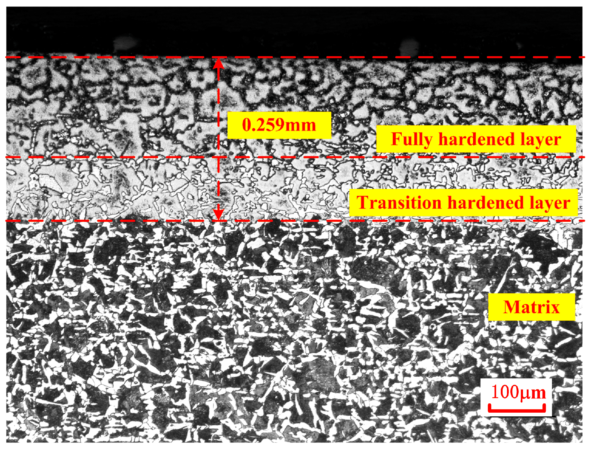
| 5 | 450 | 10 | 0.271 | 0.259 | 4.63% | |
| 6 | 450 | 6 | 0.204 | 0.219 | 6.85% | |
| 7 | 450 | 8 | 0.221 | 0.232 | 4.74% | |
| 8 | 450 | 12 | 0.283 | 0.274 | 3.28% | |
| 9 | 450 | 14 | 0.312 | 0.296 | 5.4% |
© 2020 by the authors. Licensee MDPI, Basel, Switzerland. This article is an open access article distributed under the terms and conditions of the Creative Commons Attribution (CC BY) license (http://creativecommons.org/licenses/by/4.0/).
Share and Cite
Guo, Y.; Liu, M.; Yin, M.; Yan, Y. Modeling of the Evolution of the Microstructure and the Hardness Penetration Depth for a Hypoeutectoid Steel Processed by Grind-Hardening. Metals 2020, 10, 1182. https://doi.org/10.3390/met10091182
Guo Y, Liu M, Yin M, Yan Y. Modeling of the Evolution of the Microstructure and the Hardness Penetration Depth for a Hypoeutectoid Steel Processed by Grind-Hardening. Metals. 2020; 10(9):1182. https://doi.org/10.3390/met10091182
Chicago/Turabian StyleGuo, Yu, Minghe Liu, Mingang Yin, and Yutao Yan. 2020. "Modeling of the Evolution of the Microstructure and the Hardness Penetration Depth for a Hypoeutectoid Steel Processed by Grind-Hardening" Metals 10, no. 9: 1182. https://doi.org/10.3390/met10091182
APA StyleGuo, Y., Liu, M., Yin, M., & Yan, Y. (2020). Modeling of the Evolution of the Microstructure and the Hardness Penetration Depth for a Hypoeutectoid Steel Processed by Grind-Hardening. Metals, 10(9), 1182. https://doi.org/10.3390/met10091182