Author Contributions
Conceptualization, J.-P.B. and A.J.; software, J.H. and B.D.; validation, J.H. and J.M.; resources, B.D. and J.M.; writing—original draft preparation, J.H.; writing—review and editing, J.H., J.-P.B., and A.J.; supervision, J.-P.B. and A.J. All authors have read and agreed to the published version of the manuscript.
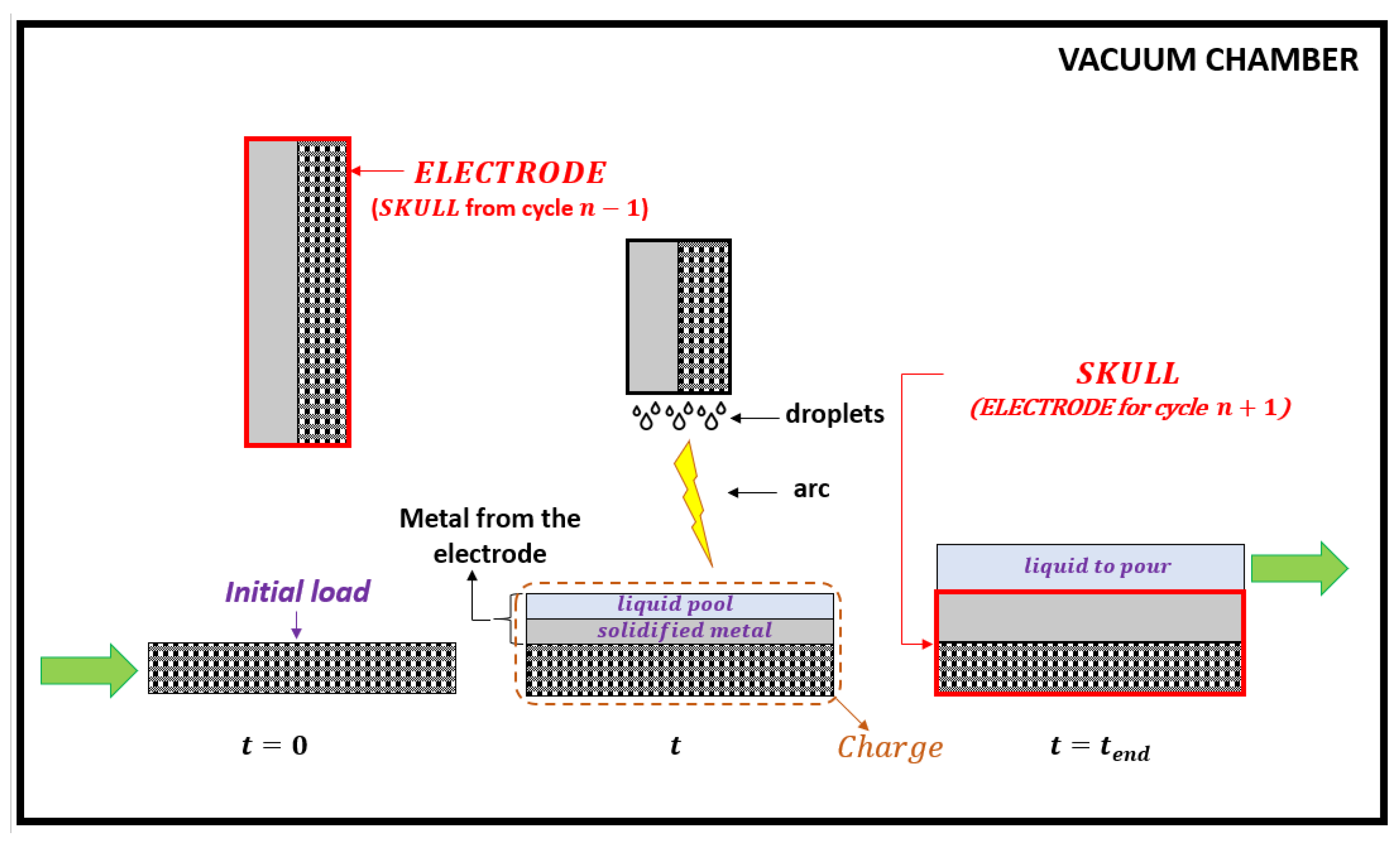
Figure 1.
Schematics of the melting cycle of the VASM process.
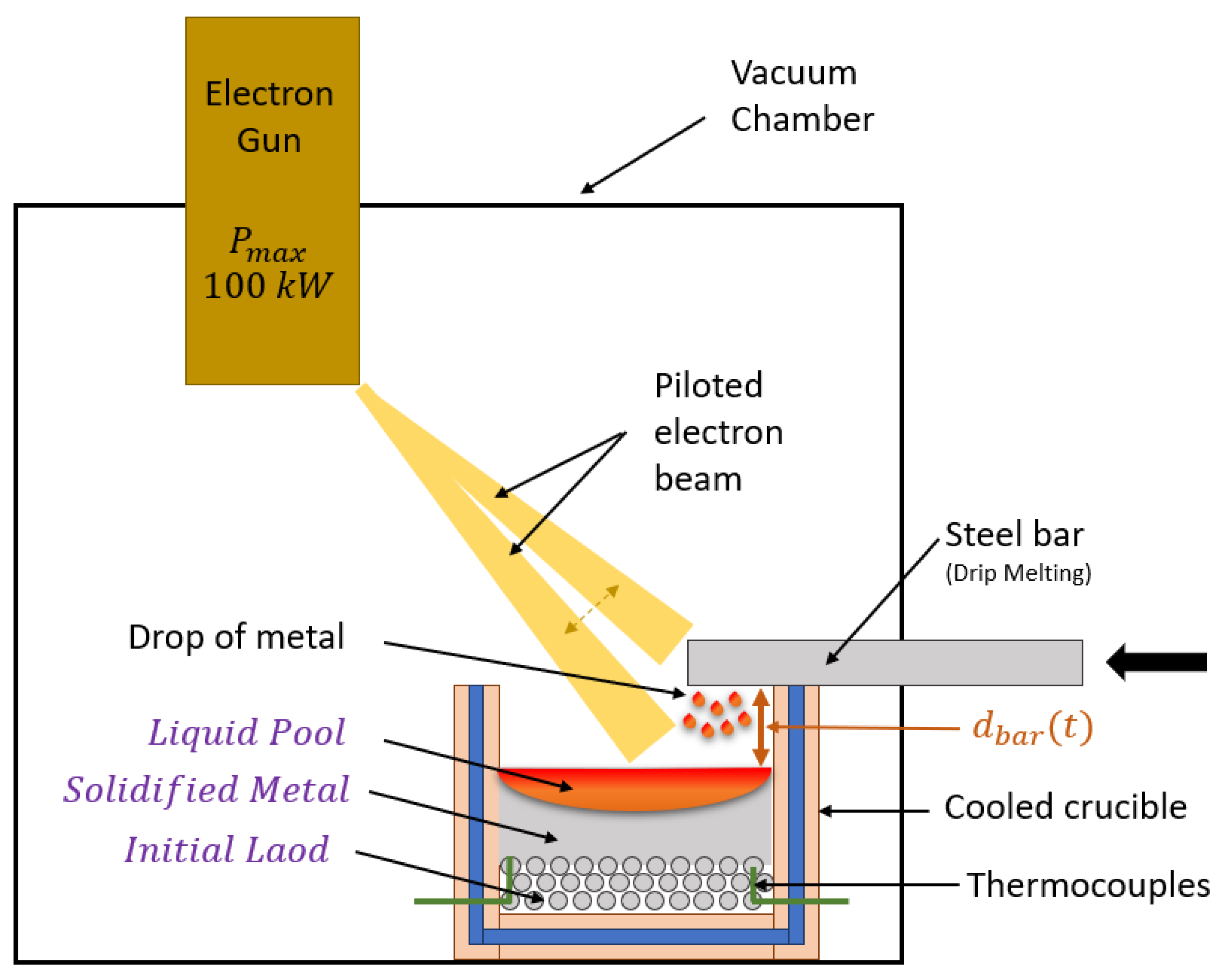
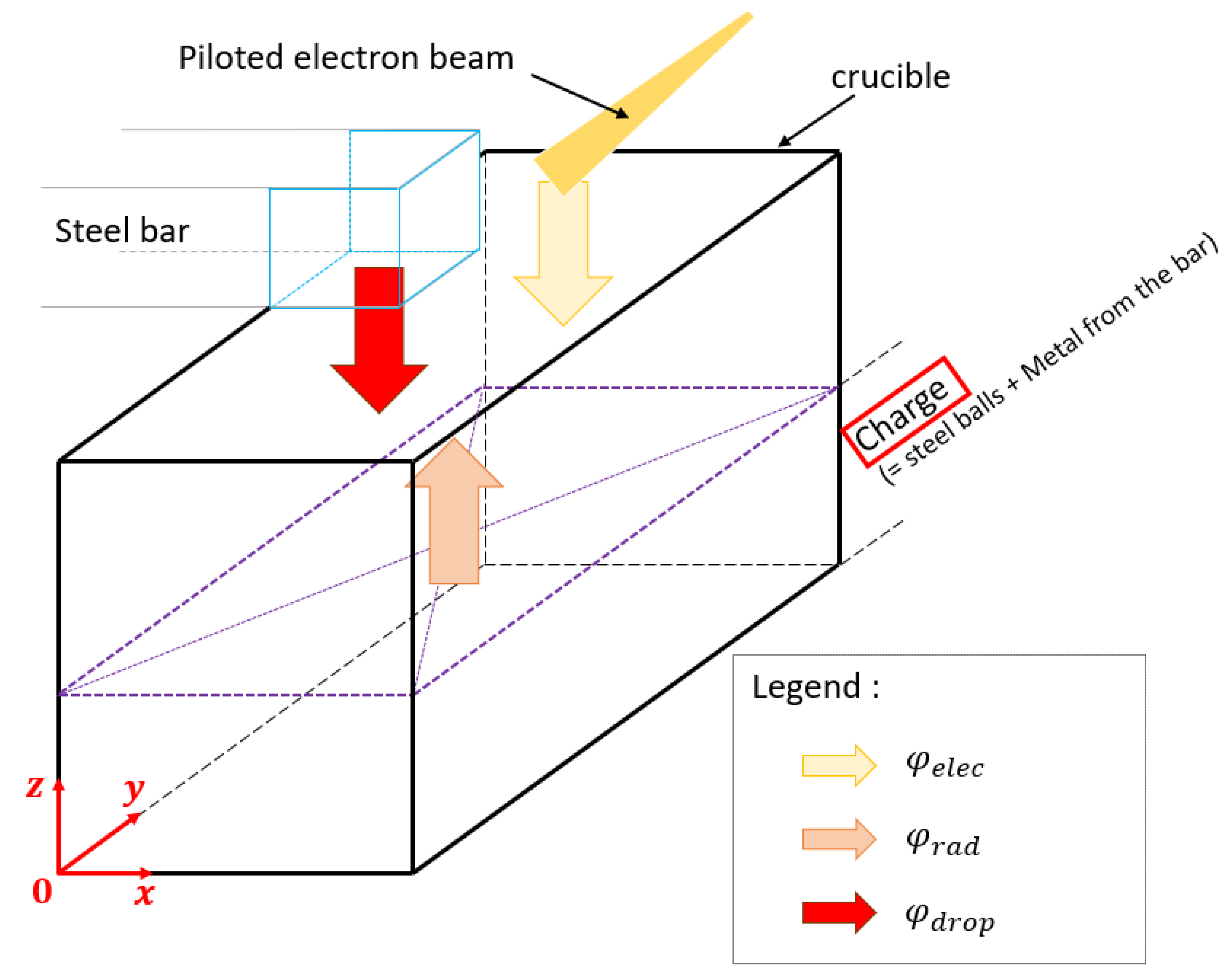
Figure 2.
Schematics of the experimental set-up.
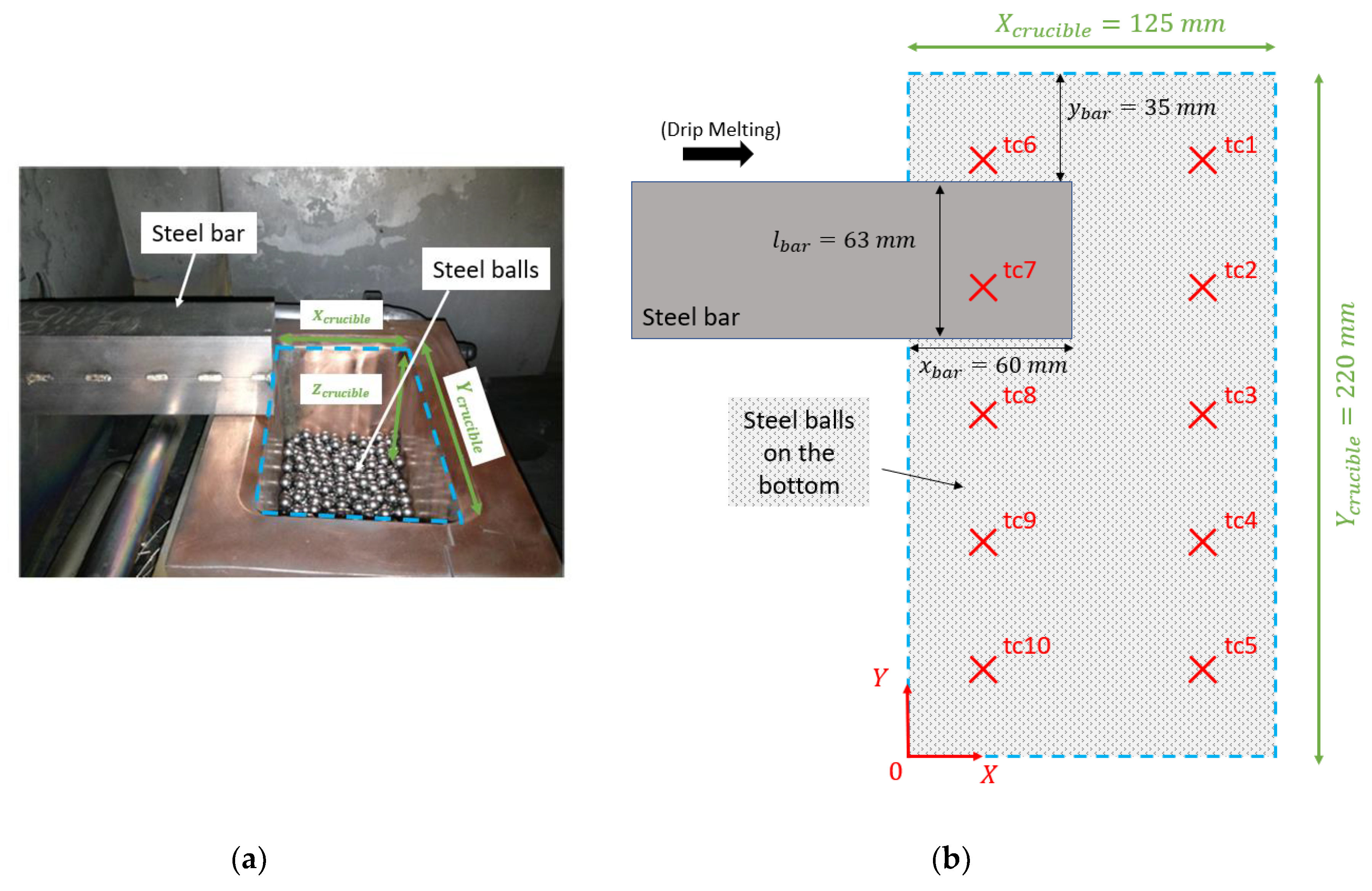
Figure 3.
Set-up of the water-cooled copper crucible. Picture of the crucible (a); top view (XY) of the crucible and locations of the thermocouples (b).
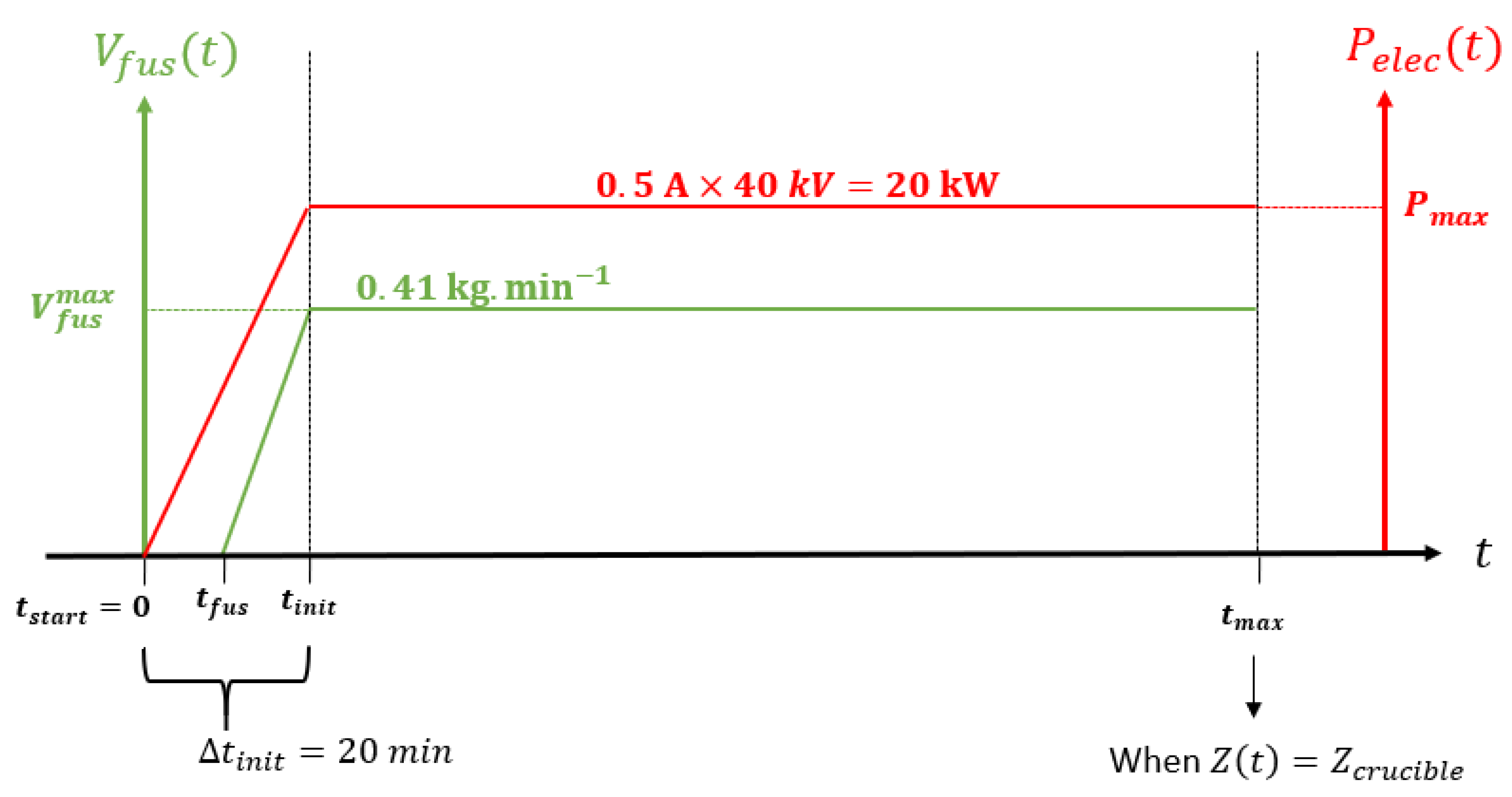
Figure 4.
Experimental electrical power and melting rate versus time.
Figure 5.
Electron beam patterns on the top of the charge.
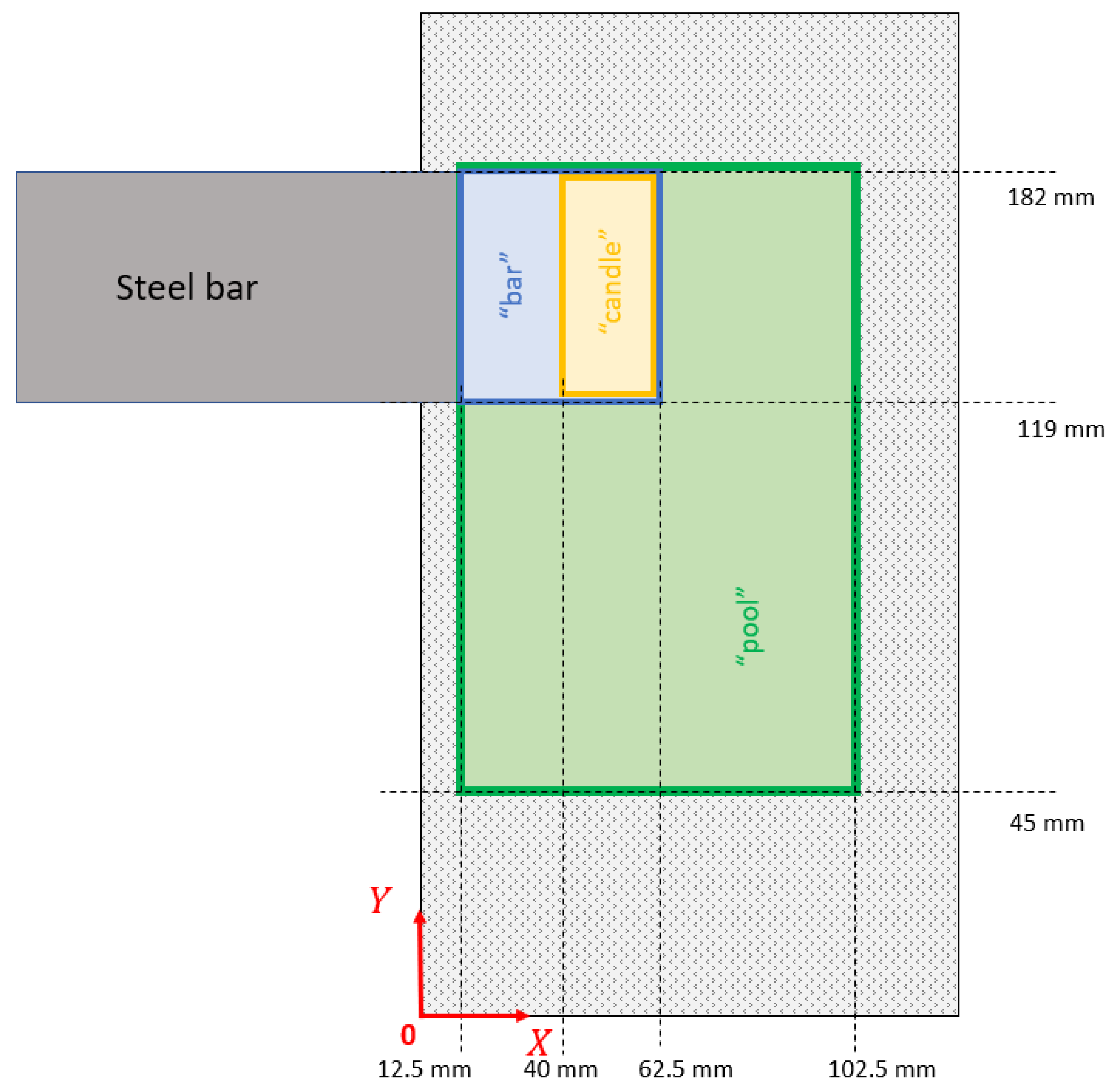
Figure 6.
Schematic of the boundary conditions at the top of the crucible.
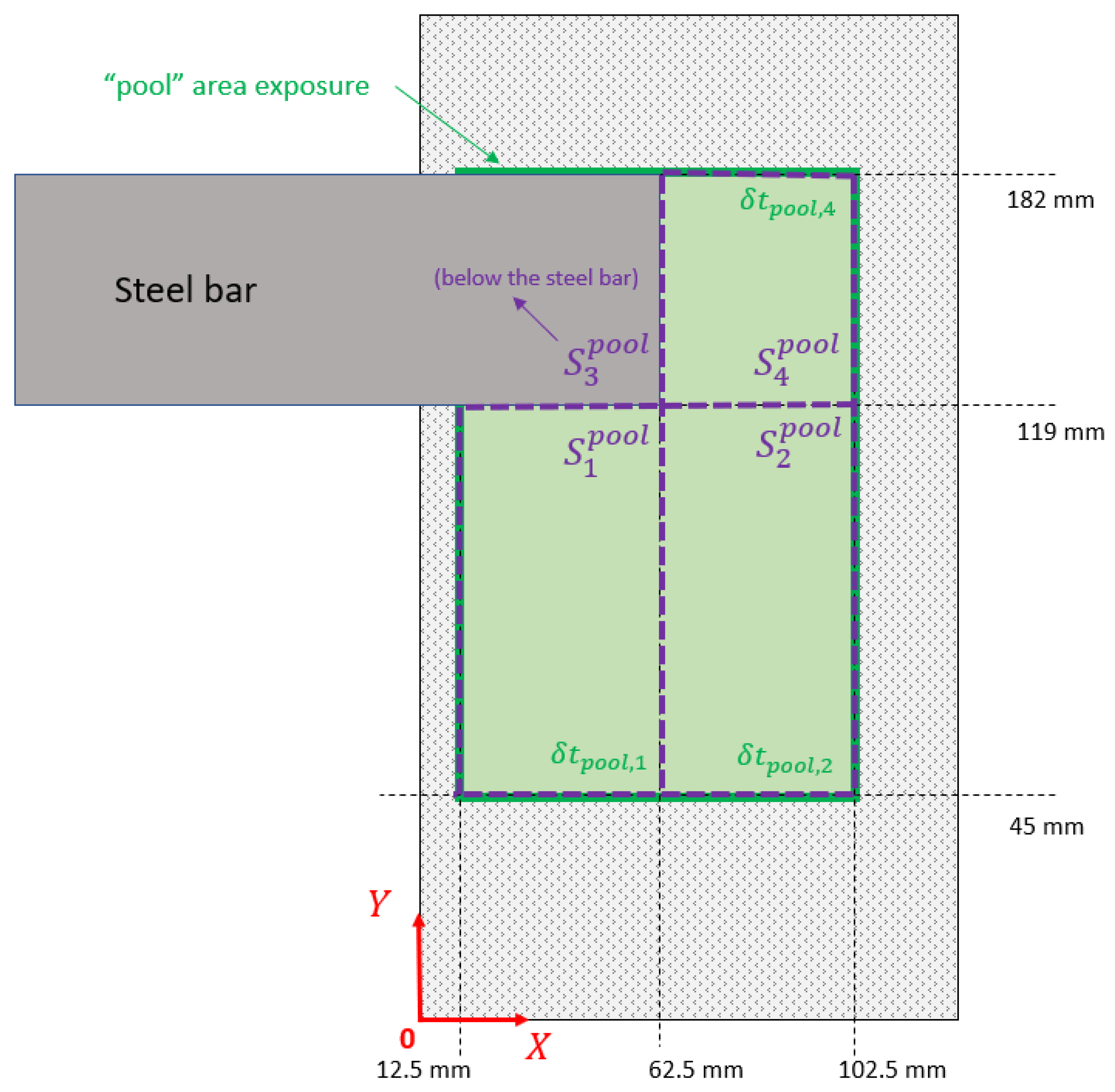
Figure 7.
Subzones of the “pool” surface.
Figure 8.
Meshing of the domain above the crucible top including the bar tip for radiative calculation purpose, the meshing of the charge is addressed in
Section 3.3.
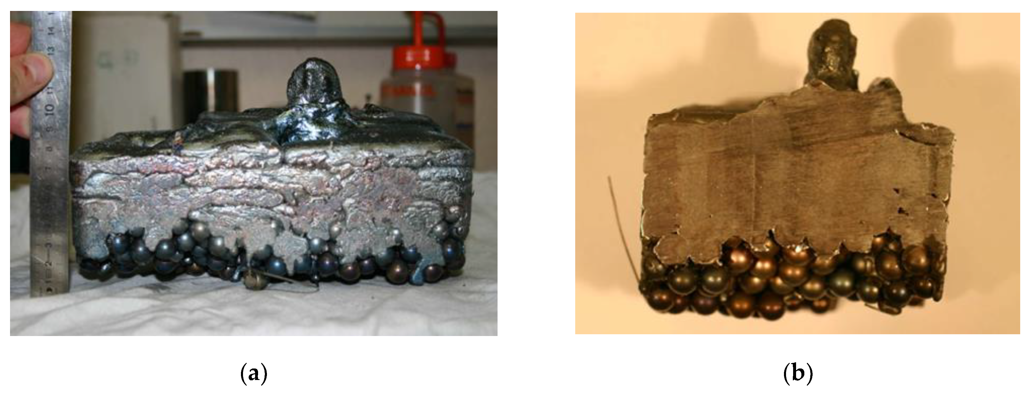
Figure 9.
Pictures of the skull after melting. (a) view from the side. (b) transverse cut.
Figure 10.
Maximum temperature calculated within the charge vs time. .
Figure 11.
Actual thermograms from thermocouples to . .
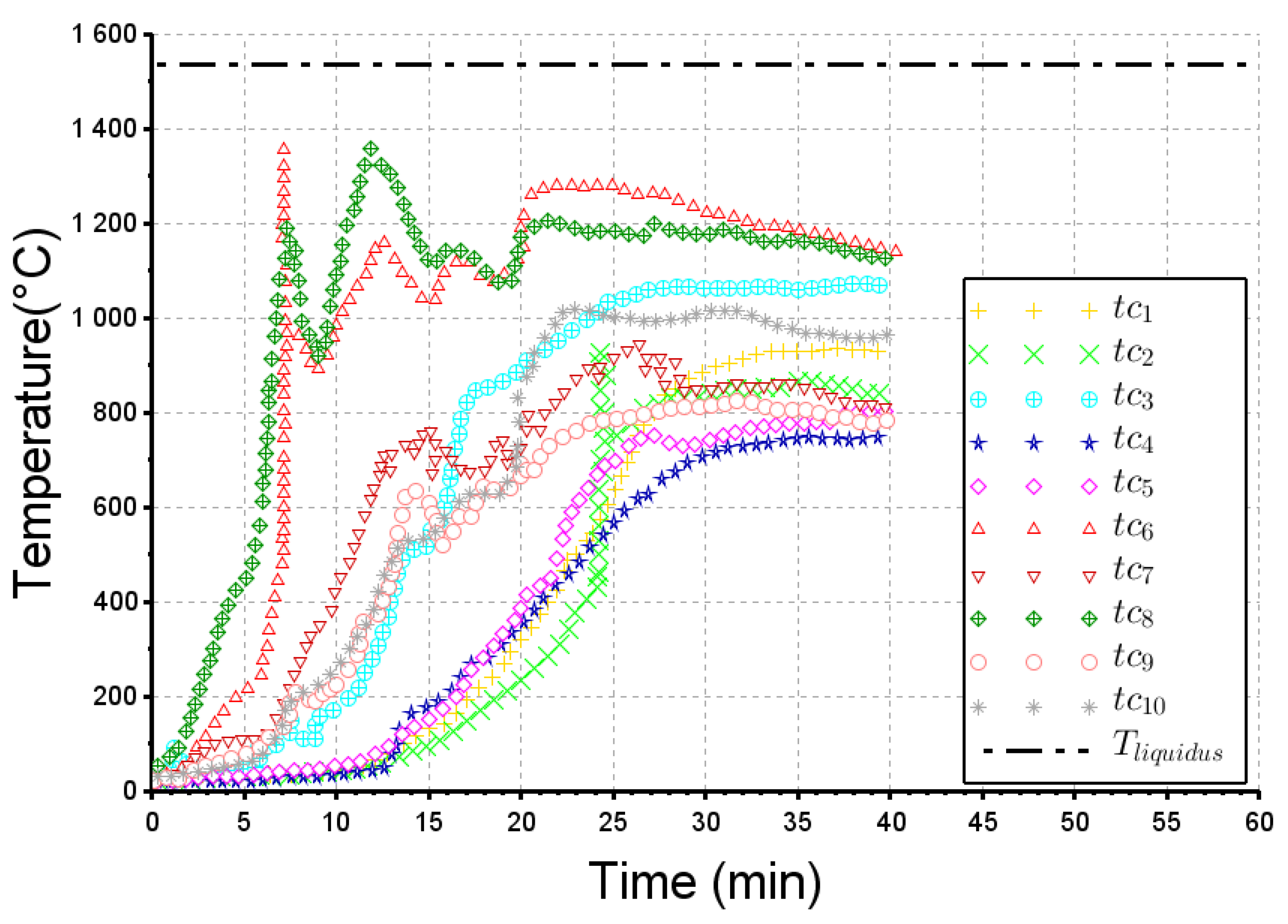
Figure 12.
Computed temperature at the location of thermocouples to . .
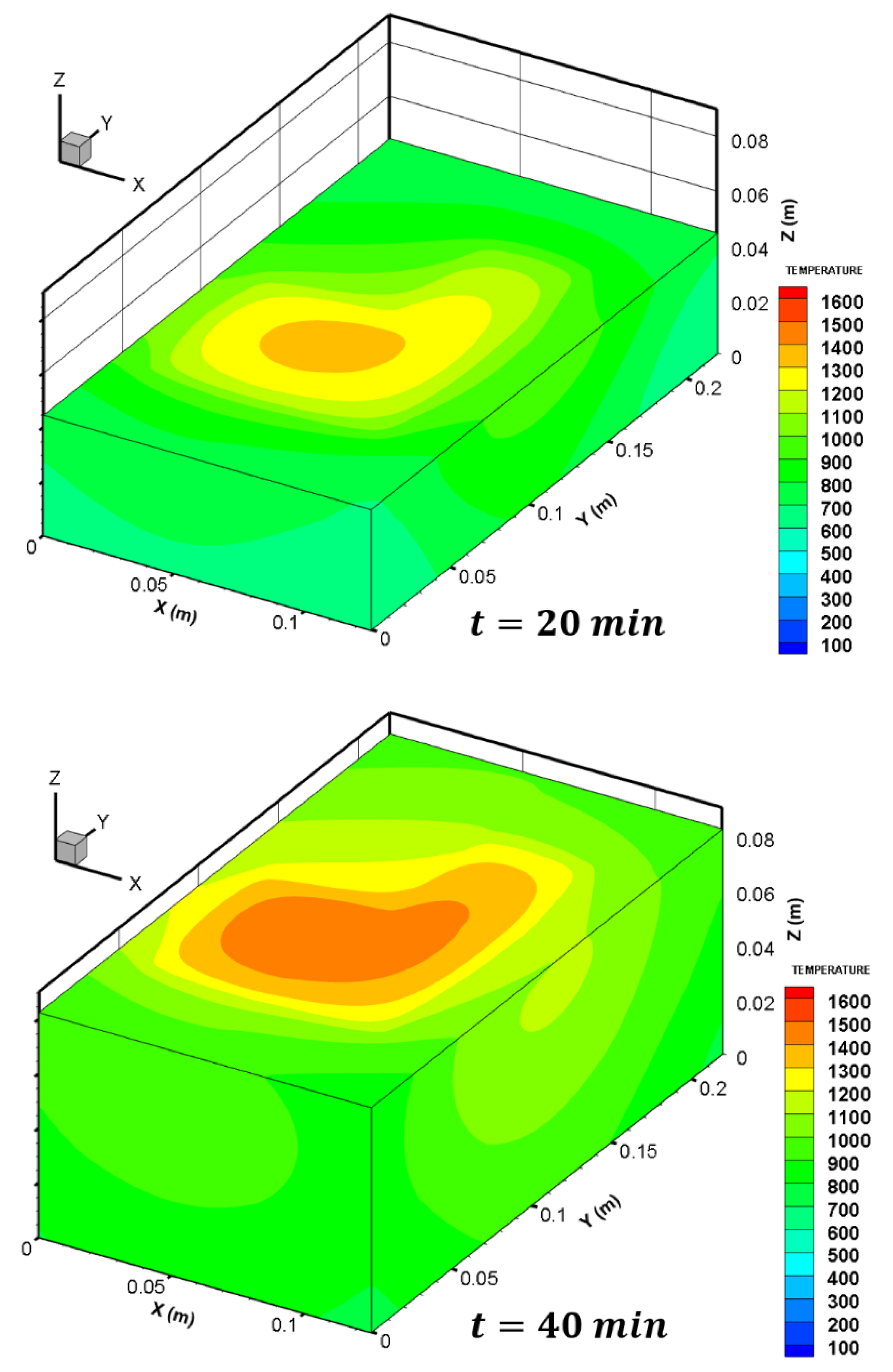
Figure 13.
Three dimensional temperature field computed within the charge at and .
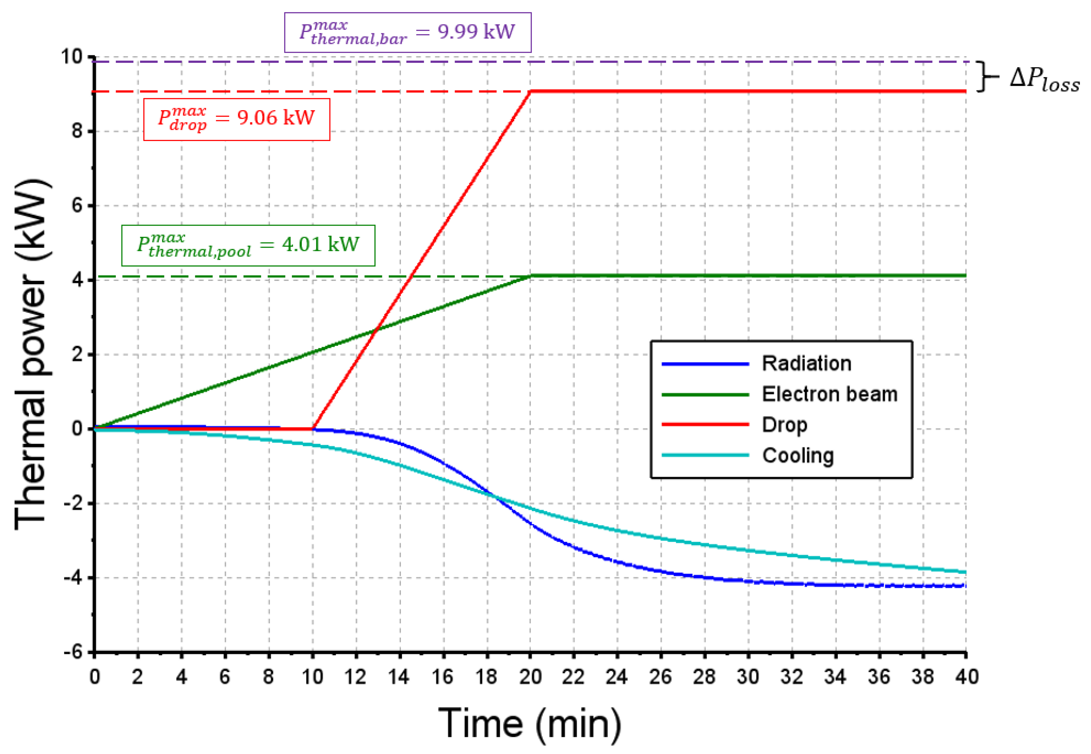
Figure 14.
Assessment of the global heat balance of the charge with time. If positive, the heat power is received by the charge.
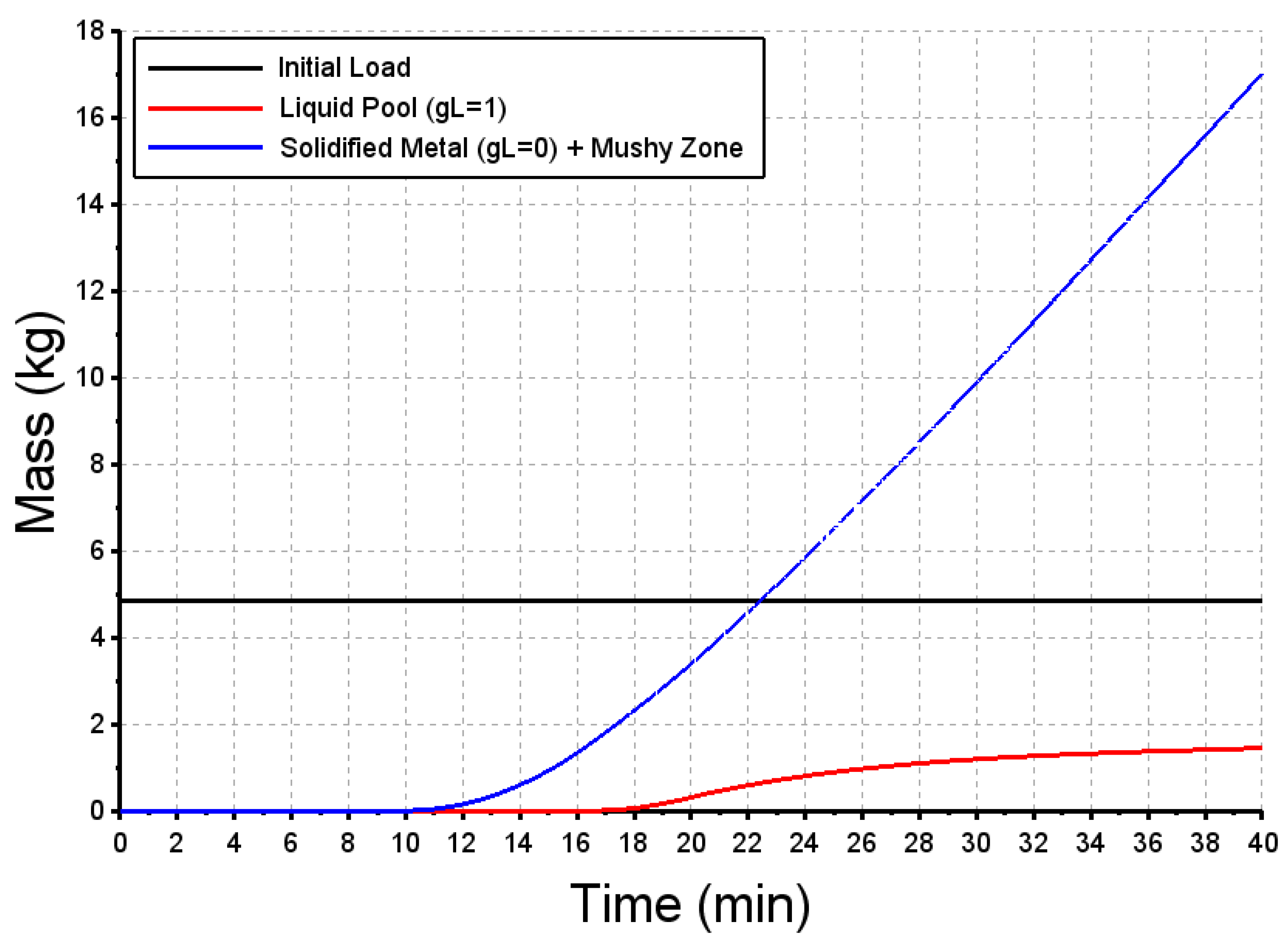
Figure 15.
Predicted mass of the initial load (in black), of the liquid pool (in red) and of the solidified metal including the mushy zone (in blue) vs time. “power+” case.
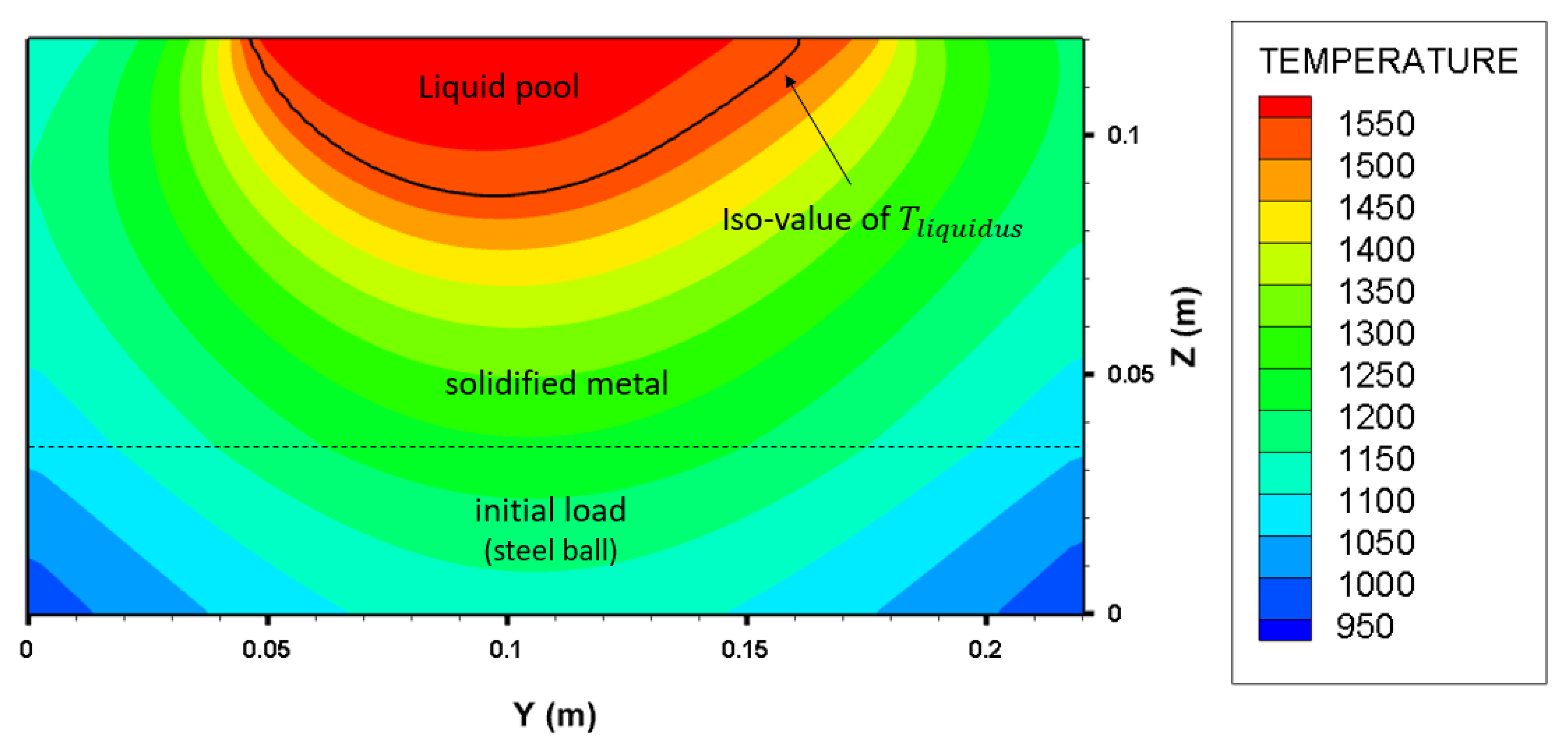
Figure 16.
Computed cross-section of the crucible () at the end of melting (t = 40 min), showing the initial load, solidified steel and liquid pool predicted by the numerical model. “power+” case.
Table 1.
Locations of the thermocouples.
| Thermocouple | X (cm) | Y (cm) | Z (cm) |
|---|
| tc1 | 10 | 16 | 2 |
| tc2 | 10 | 13.5 | 1 |
| tc3 | 11 | 11 | 3 |
| tc4 | 10.6 | 8.5 | 1 |
| tc5 | 10.2 | 6 | 2 |
| tc6 | 2.2 | 16 | 2 |
| tc7 | 2 | 13.5 | 1 |
| tc8 | 1.5 | 11 | 3 |
| tc9 | 1.7 | 8.5 | 1 |
| tc10 | 2.1 | 6 | 2 |
Table 2.
Exposure time of the electron beam on each surface “pool”, “bar” and “candle”, and corresponding thermal power and flux density.
| Pool | Bar | Candle |
|---|
| Exposure time | | | |
| Thermal power | 5.38 | 4.31 | 4.31 |
| Area | 12,330 mm2 | 3150 mm2 | 1417.5 mm2 |
| Thermal flux density | 436.3 mm2 | 1368.3 mm2 | 3040.6 mm2 |
Table 3.
Expressions of , and depending on which phase is the metal.
| Metal Phase | | | |
|---|
| Liquid Pool | | | |
| Mushy zone | | | |
| Solidified metal | | | |
| Initial load | | | |
Table 4.
Exposure time according to the subzone .
| | | | |
|---|
| Area | 3700 mm2 | 2960 mm2 | mm2 | mm2 |
| of “pool” area | | | | |
| | | shadow | |
Table 5.
Thermodynamic values of steel alloy, data from [
19].
| |
| |
| |
| |
| |
| |
| |
| |
| |
Table 6.
Heat thermal balance at t = 40 min.
| Thermal power of the EB (kW) | 14.0 | 100% |
| Thermal power lost by the steel bar (radiation) (kW) | 0.9 | 6.4% |
| Thermal power lost by the charge (water cooling and radiation) (kW) | 8.0 | 57.1% |
| Heating power of the charge (kW) | 5.1 | 36.5% |
Table 7.
New operating conditions compared to the reference case.
| Configuration | | | | | |
|---|
| “reference” | | | | | |
| “power+” | | | | | |
Table 8.
Masses of the three parts of the charge at t = 40 min (“power+” case).
| Total (kg) | 23.3 | 100% |
| Mass of the initial load made of steel balls (kg) | 4.8 | 20.6% |
| Mass of the solidified and mushy metal (kg) | 17.0 | 73.0% |
| Mass of the liquid pool (kg) | 1.5 | 6.4% |
Table 9.
Heat thermal balance at t = 40 min (power+ case).
| Thermal power of the EB (kW) | 25.2 | 100% |
| Thermal power lost by the steel bar (radiation) (kW) | 1.6 | 6.3% |
| Thermal power lost by the charge (water cooling and radiation) (kW) | 13.2 | 52.4% |
| Heating power of the charge (kW) | 10.4 | 41.3% |


