Application of the Cumulative Kinetic Model in the Comminution of Critical Metal Ores

Abstract

Over the last decades, several reliable mathematical models have been developed for simulating ore comminution processes and determining the Work Index. Since Fred Chester Bond developed the Work Index standard procedure in 1961, numerous attempts have been made to find simpler, faster, and economically more advantageous alternative tests. In this paper, a Bond test simulation based on the cumulative kinetic model (CKM) has been checked on a spreadsheet. The research has been accomplished by conventionally determining the kinetic parameters for some Ag and Au ores and for three pure minerals and one rock that are common constituents of the gangue rock. Analysis of the results obtained allowed to develop a simplified procedure for calculating the kinetic parameters and their application to Work Index determination through simulation.

1. Introduction

Energy consumption during the comminution stage has a severe impact on the operational costs of ore processing plants, being a key factor in operation planning and optimization. This situation has drawn the interest of researchers on early stages of ore processing, who tie the amount of energy consumed with the work done in the comminution of the mineral species involved.

The First Law of Comminution or Rittinger’s Law [1] dates back to 1867 and postulates that the energy required in the mineral breakage is directly proportional to the new surface area produced. Later, in 1885, the Second Law of Comminution was postulated by Kick [2], who stated that the energy supplied is proportional to the particle volume, regardless of the original size. In 1952, Fred Chester Bond [3,4] postulated the Third Law of Comminution (also known as Bond’s Law). It states that the energy required is proportional to the length of crack initiating breakage. However, as mentioned by Jankovic et al. [5], the application of Kick’s and Rittinger’s laws has been met with varied success and are not realistic for designing size reduction circuits, while Bond’s Third Law can be reasonably applied to the range in which ball/rod mills operate. In spite of its empirical basis, Bond’s Law is the most widely used method for the sizing of ball/rod mills and has become a standard. Nevertheless, despite being unrivalled, it has an error range of up to 20%. Besides, determining the Work Index (wi) for a given mineral or ore composition is a time-consuming procedure that requires qualified personnel and a significant quantity of sample [6,7,8].

These drawbacks were resolved to some extent by several researchers, who developed alternative methodologies to determine energy consumption during crushing and grinding [9,10,11,12,13,14,15]. Some methodologies [7,16,17,18,19,20] employed mathematical simulations based on tested mathematical models. In all cases, they involve an adequate characterization of the material in the laboratory, followed by the simulation of the grinding and sorting operations of the standard test to determine the Work Index (w_i).

The cumulative kinetic model (CKM) was developed by Laplante et al. [21], and it represents a simple solution to the basic equation proposed by Loveday [22]. As Menéndez-Aguado [8] pointed out, it possesses several advantages, the main of which are that the model is defined by two parameters, simplifying the interpretation of the results and that the parameters determined in the laboratory can be applied at industrial scale [23].

2. Theoretical Background

2.1. The Cumulative Based Kinetic Model

The CKM is based in a first-order kinetic equation, in which the particle breakage rate for a given particle size interval is proportional to the mass existing in that interval. It has the particularity of being defined in terms of only two parameters, which may be determined in laboratory batch tests and then directly applied to the model.

The kinetic parameter (k) is defined as the oversize disappearing rate for a given size class, either at continuous or discontinuous grinding under a piston flow regime, and can be described as shown in Equation (1).

$$W_{\left(x,t\right)}=W_{\left(x,0\right)}\exp \left(-k t\right)$$

(1)

where

W(x,t) = cumulative percent of oversize for size class x in time t.

W(x,0) = cumulative percent of oversize for size class x at the feed.

k = breakage rate constant (min⁻¹)

t = time (min).

The relationship between breakage velocity and particle size is shown in Equation (2):

$$k=C x^n$$

(2)

In Equation (2), C and n are constants depending on the features of the mineral and the mill, as described by Ersayin et al. [24]. They are CKM model parameters and can be determined experimentally. Provided that size distribution in the feed stream is known, C and n allow to calculate the size distribution of the product through Equation (3).

$$W_{\left(x,t\right)}=W_{\left(x,0\right)}\left(\exp \left(-C x^n t\right)\right)$$

(3)

2.2. Determination of the CKM Parameters C and n

Parameters C and n may be calculated simply and quickly from a small amount of sample in a laboratory mill [8]. In our case, since the objective was simulating the Bond tests to obtain w_i, the standard mill designed by Bond was used for characterization purposes.

Keeping the same feed quantity as in Bond test (700 cm³), successive grinding cycles were done at predefined time intervals. After each cycle, a representative sample of the mineral load was extracted, and its particle size distribution (PSD) was obtained. The part of the sample above the reference size was then conveyed back to the mill and new feed was added up to the initial load before resuming the test.

The k values are calculated for several monosizes through linear regression of the retained mass accumulated for each grinding time, using the Equation (1) linearized:

$$\ln \left(W_{\left(x,t\right)}\right)-\ln \left(W_{\left(x,0\right)}\right)=k t$$

(4)

Linearizing Equation (2) and performing a new linear regression for each monosize, C and n are obtained:

$$\ln \left(k\right)=\ln \left(C\right)+n \ln \left(x\right)$$

(5)

Taking into account that Equation (5) is the equation of a straight line, ln(C) is the intercept on the y-axis and n is the slope. Thus, the parameters are set for applying Equation (3) to obtain the size distribution as a function of grinding time.

2.3. Simplified Procedure to Grinding Kinetic Parameters Determination

Figure 1 shows the outcome of Equation (4) as a function of grinding times for monosizes of 840, 420, 149, and 53 µm of a pure quartz sample. It can be seen that the slope (k) remains rather constant irrespective of the time considered, from intermediate values to the end (5 min) of the test. A reduction of the test duration would be important to obtain the kinetic parameters through this procedure.

To check this procedure, this work was aimed at validating the proposed methodology to determine the grinding kinetic parameters. The modelling was then used to determine the Work Index through simulation, and finally, those results were compared for eight different samples with the w_i obtained through the Bond standard test.

3. Methodology

3.1. Sample Preparation

Eight samples were selected, of which four, namely, M1S1, M2S1, M2S2, and M2S3, were critical metal ores (Ag and Au) and the rest consisted of minerals (feldspar, quartz, and calcite) and a rock (pure limestone), being usual constituents of gangue rock.

It must be taken into account that critical metal ores have commonly a very low grade, and thus, it is the gangue composition that defines their grindability behavior.

Heretofore, M1S1 stands for a hydrothermal low sulfidation mineral ore, consisting of veins and veinlets of silica (quartz, chalcedony, and opal) containing free gold, electrum, and Ag sulfosalts, in addition to cassiterite, galena, pyrite, and chalcopyrite. M2S1, M2S2, and M2S3 stand for an interpreted medium-sulfidation epithermal system, containing quartz, carbonates, and, to a lesser extent, Ag-, Au-, Pb-, Cu-, and Zn-bearing sulfides and sulfosalts.

Sample preparation was done following the usual procedures for the standard Bond test [4]: progressive comminution through several steps in jaw crusher, cone crusher, and roll/roller mills, until a final product finer than 6 mesh (3.35 mm) is obtained, avoiding an over-representation of the finest fraction.

The samples finer than 6 mesh were then subsampled with a rotary splitter. The resulting subsamples, 1 kg each approximately, were used in mineralogical, chemical, and grain size characterization and also constituted the feed and the fractions for the Bond and grinding kinetic tests.

Grain size analyses were performed after sieving, approximately 300 g of each sample in a RO-TAP Sieve Shaker using a series of ASTM sieves.

3.2. Work Index Determination

The Bond test for ball mills was performed for each sample following the abovementioned Bond standard procedure [4]. The resulting value was later used as a reference to compare with the Work Index obtained through simulation. An initial feeding sample with a volume of 700 cm³ was weighed and then fed into the standard mill filled up with the ball load defined for the test. After a grinding period of an arbitrary number of revolutions (e.g., 100), the mill was carefully dumped, recovering the maximum possible of the fines from the ball charge and the mill liners to minimize sample losses. The material was sieved to the reference size (P₁₀₀), and the undersize was weighed. An equal mass of new raw material was then added to the oversize feed to compensate loss of the fines.

The process was repeated, weighing the newly produced undersize (G) concerning the reference mesh. This undersize (G) was divided by the number of revolutions resulting in the grams per revolution (Gbp). Once Gbp is known, a new grinding cycle was performed after calculation of the needed revolutions to reach the steady state. The cycle was repeated until the undersize produced per revolution (Gbp) came to an equilibrium and the circulating feed approached 250%. The Gbp of the two last cycles was then averaged to obtain the grindability index of the test. The P₈₀ of the undersize to the reference size was obtained allowing the calculation of the Work Index with Equation (6).

$$w_i=\frac{44.5}{P_{100}^{0.23}Gb{p}^{0.82}\left[\frac{10}{\sqrt{P_{80}}}-\frac{10}{\sqrt{F_{80}}}\right]}$$

(6)

where

w_i = Bond Work Index (kWh/sht).

P₁₀₀ = test reference size (µm).

Gbp = Grindability Index for the mineral (g/rev.).

F₈₀ = grain size corresponding to 80% of the feed undersize (µm).

P₈₀ = grain size corresponding to 80% of the final undersize (µm).

Regarding w_i units, although the original Bond formulation uses short tons (sht), results from this work are given in metric tons, after applying the corresponding conversion factor.

3.3. Determination of the Kinetic Parameters

As mentioned before, the kinetic parameters (C and n) were determined in a Bond standard mill with its corresponding ball charge to avoid variability. According to Ersayin et al. [24], the parameters C and n are a function of both the mineral and mill features.

The test feed was a 700 cm³ representative sample with known particle size distribution. Several grinding runs were performed with different cumulative times (0.5, 1, 2, 3, 4, and 5 min). Size analysis was done between runs, the analyzed sample being reintroduced into the mill before resuming the process. Size analyses were then used first to determine the constant k and then the parameters C and n for each time and size class, using Equations (4) and (5).

3.4. Simulation Based on the Cumulative Kinetic Model

The cumulative kinetic model provides the size distribution of the product from the size distribution of the feed and the grinding times, using Equation (3) and the parameters C and n, determined in the laboratory.

As in the Bond test, an arbitrary initial number of revolutions was set and converted into time units (provided that the mill speed is 70 rpm). Then, using Equation (3), the quantity of product for a reference particle size was calculated. By comparing with the weight of the feed, the resulting undersize and the Gbp were determined for the cycle.

The simulator calculates the new feed (weight and PSD) from the reference size reject of the previous cycle plus the fresh feed that replaces the undersize product of the previous cycle. Next, it calculates the number of revolutions for the following cycle and the grain size distribution of the reconstituted feed. The cycle is repeated until Gbp stability is reached and a circulating load is close to 250%. Finally, the simulation ends after calculating the simulated Work Index value (w_is).

A spreadsheet for performing the simulation is available as Supplementary data.

4. Results

4.1. Simulation of the Work Index, Obtaining the Kinetic Parameters through the Conventional Procedure

Table 1. Comparison between Work Indexes for pure gangue components and reference size 100 µm, obtained through the standard procedure and the simulation (w_i = Work Index; w_is = simulated Work Index).

Ore	Kinetic Parameters		R2	wis (kWh/t)	wi (kWh/t)	Difference (%)
	C	n
Feldspar @100 µm	0.000586	1.07	0.98	11.67	12.41	6.0
Limestone @100 µm	0.001789	0.87	0.97	9.66	9.98	3.2
Calcite @100 µm	0.000973	1.09	0.95	6.41	6.30	−1.7
Quartz @100 µm	0.000448	1.07	0.99	13.77	13.88	0.8

displays the results obtained for the studied usual components of the gangue. It includes the kinetic parameters, the Work Index for the Bond standard procedure, and the Work Index obtained through simulation. The latter two were obtained for a reference size of 100 µm.

Table 2. Comparison between Work Indexes for metal ores and reference mesh of 100 µm, obtained through the standard procedure and the simulation (w_i = Work Index; w_is = simulated Work Index).

Ore	Kinetic Parameters		R2	wis (kWh/t)	wi (kWh/t)	Difference (%)
	C	n
M1S1 @100 µm	0.000792	0.89	0.99	19.56	19.25	1.6
M2S1 @100 µm	0.000451	1.03	0.98	15.55	14.83	−4.9
M2S2 @100 µm	0.000486	1.03	0.98	16.61	15.98	3.8
M2S3 @100 µm	0.000303	1.10	0.99	17.06	17.35	−1.7

displays the results obtained for the critical metal ores studied. It includes the kinetic parameters and Work Indexes obtained through Bond standard procedure and simulation (reference size of 100 µm).

Bond index values were also determined, with a 150 µm reference size, for feldspar and quartz and then compared with those determined through simulation using CKM.

Table 3. Work Indexes for feldspar and quartz (reference sizes 100 and 150 µm) obtained through the standard test and the simulation (w_i = Work Index; w_is = simulated Work Index).

Ore	Kinetic Parameters		R2	wis (kWh/t)	wi (kWh/t)	Difference (%)
	C	n
Feldspar @150 µm	0.000586	1.07	0.98	11.67	12.41	6.0
Feldspar @100 µm				14.19	14.69	3.4
Quartz @150 µm	0.000448	1.07	0.99	13.77	13.88	0.8
Quartz @100 µm				17.34	17.88	3.0

compares the results obtained through the standard procedure and the simulation for both minerals. It was noted that the differences between w_i and w_is for 150 µm were within the range obtained in the previous cases for a reference size of 100 µm.

4.2. Work Index Determination by Obtaining the Kinetic Parameters through the Simplified Procedure

From the results of the tests carried out to determine the kinetic parameters for each sample, it the product size distribution of the longest grinding time test was selected. Then, the slope was determined from the starting time to the end time of the test to obtain k for all the grain size populations involved.

To calculate C and n, the condition was set of using the widest grain size range, with an upper (coarsest) limit of 840 µm and including the finest possible populations without distorting the outcomes significantly. For most cases, this resulted in a lower (finest) limit of 53 µm.

Table 4. Compared results between w_i and w_is using the simplified procedure to obtain the kinetic parameters.

Ore	Size Interval (µm)		Grinding Time (min)	wi (kWh/t)		Difference (%)
	Minimum	Maximum		Real	Simulated
Feldspar @100 µm	53	840	0–4	14.69	13.38	8.91
Feldspar @150 µm	53	840	0–4	12.41	11.20	9.76
Quartz @100 µm	53	840	0–5	17.88	17.82	0.33
Quartz @150 µm	53	840	0–5	13.88	14.63	−5.37
Limestone @100 µm	53	840	0–4	9.98	9.41	5.72
Calcite @100 µm	53	840	0–4	6.30	6.24	0.96
M1S1 @100 µm	74	840	0–3	19.25	21.11	−9.68
M2S1 @100 µm	53	840	0–3	14.83	15.40	−3.85
M2S2 @100 µm	74	840	0–3	15.98	17.01	−6.47
M2S3 @ 100 µm	53	840	0–3	17.35	16.79	3.21

displays a comparison of the Work Indexes obtained through the Bond standard test and the simulation using the kinetic parameters provided by the simplified procedure. It can be seen that Work Indexes from the simulation using the simplified procedure differ from those from the Bond standard procedure by less than 10%.

5. Discussion

The simulation of the Work Index test applying the cumulative kinetic model proved to yield results that differ by less than 10% from those from the Bond standard test. This figure agrees with results by Ahmadi and Shahsavari 2009 [25], who proposed a two-step simplified procedure. They applied a simulation based on the cumulative kinetic model and validated their results over three samples of iron ore and one of copper ore. Their results differed by less than 7% from those yielded by the standard procedure. Previously, Aksani and Sönmez 2000 [7] determined the Bond indexes by means of the cumulative kinetic model with values differing by less than 4% with respect those determined with the standard test.

As to determining the kinetic parameters, the possibility of reducing the procedure to only one grinding test with the greatest possible estimated time to obtain the grain size distribution over which the k index and then the parameters C and n could be calculated was evaluated.

As it can be observed in the graph of Figure 1, illustrating the tests performed with quartz, the slope for each particle size class does not vary much over the time span recorded. This suggests that the determination of the constant k would not require obtaining grain size data at intermediate grinding times.

The graph of Figure 2 shows that k values vary for different particle sizes over the grinding time. For grinding times longer than 3 min, the curve is straight for the grain size class between 595 and 840 µm (20 and 30 mesh), and then after a break in slope, a straight line continues again. It can also be noticed that, with grinding time, the different curves adjust and merge into a new slope.

A similar situation occurs for the remaining studied minerals, as the graph of Figure 3 depicts. This graph shows the variation of k with particle size according to grinding times of feldspar. Similarly, Figure 4 displays the results for the ore M2S2.

The graphs show that the curves display a stable shape after a given grinding time. In all cases, a change in slope takes place for particle size coarser than 700 µm. That is the reason why the simplified procedure should not be extended for particle sizes coarser than 840 µm. (20 mesh). This condition does not involve an important limitation since this is the usual particle size range employed in ball mill grinding.

Indeed, it was decided to use the maximum time employed in for each mineral grinding, highlighting the convenience of using a grinding time of at least 5 min to calculate the kinetic parameters with this procedure.

It can be considered that the simplified procedure permits to determine the grinding kinetic parameters C and n, after carrying out one grinding test and two PSD analyses. This can be done rapidly in the laboratory once the sample is prepared. It is considered a valid procedure for a particle size range between 840 and 53 µm with a grinding time of 5 min, using the standard Bond mill with the standard ball charge. The procedure can be summarized as follows:

(1)

Feed preparation 100% passing a 3350 µm (6 mesh) sieve followed by gradual crushing to avoid the overproduction of fines.

(2)

PSD determination with sieves between 3350 and 37 µm, and determination of the feed characteristic particle size (F₈₀).

(3)

Grinding of a quantity equivalent to 700 cm³ for 5 min.

(4)

PSD analysis to determine the product characteristic particle size (P₈₀).

(5)

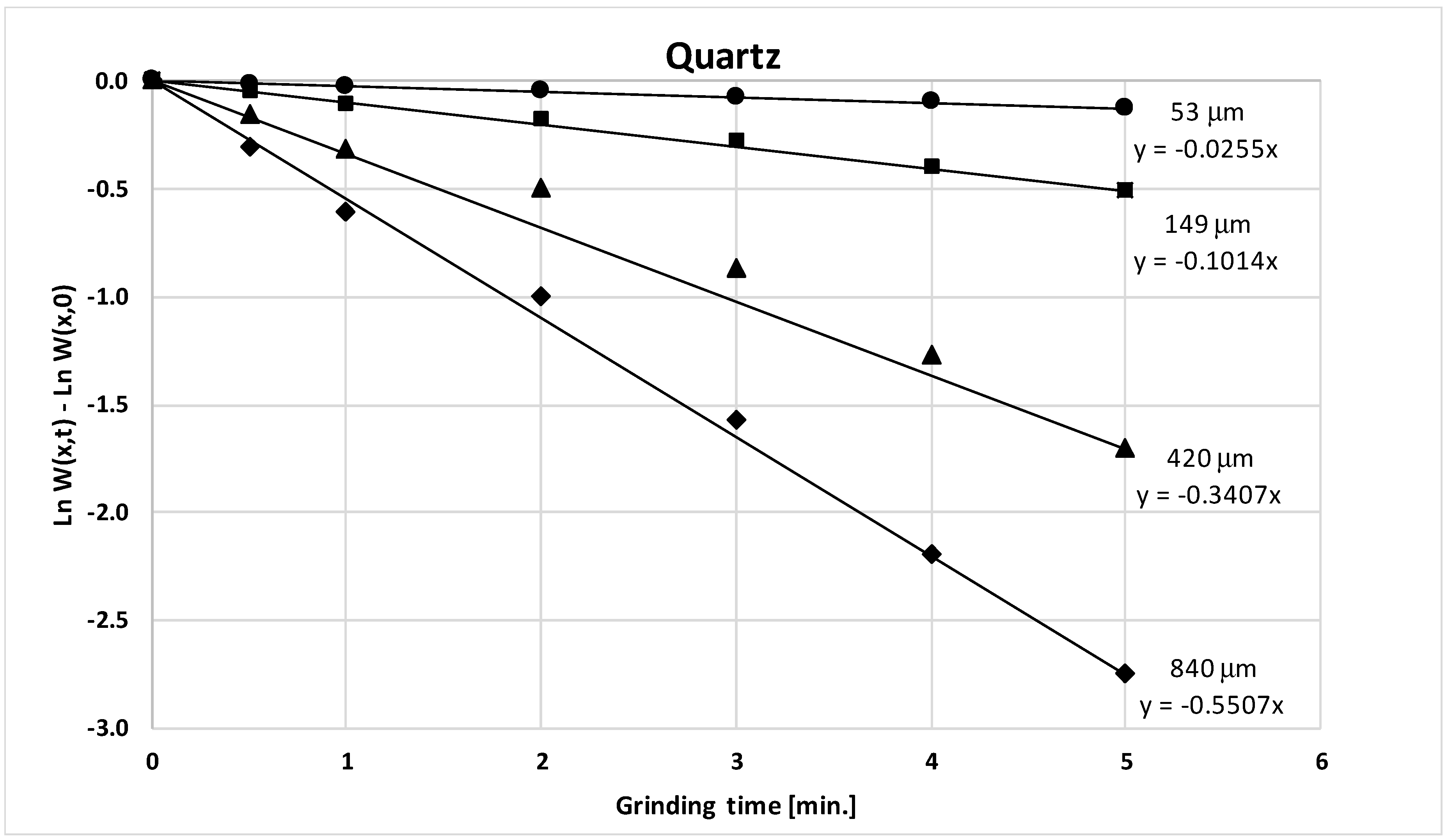
Determination of k for each particle size class (slope from 0 to 5 min).

(6)

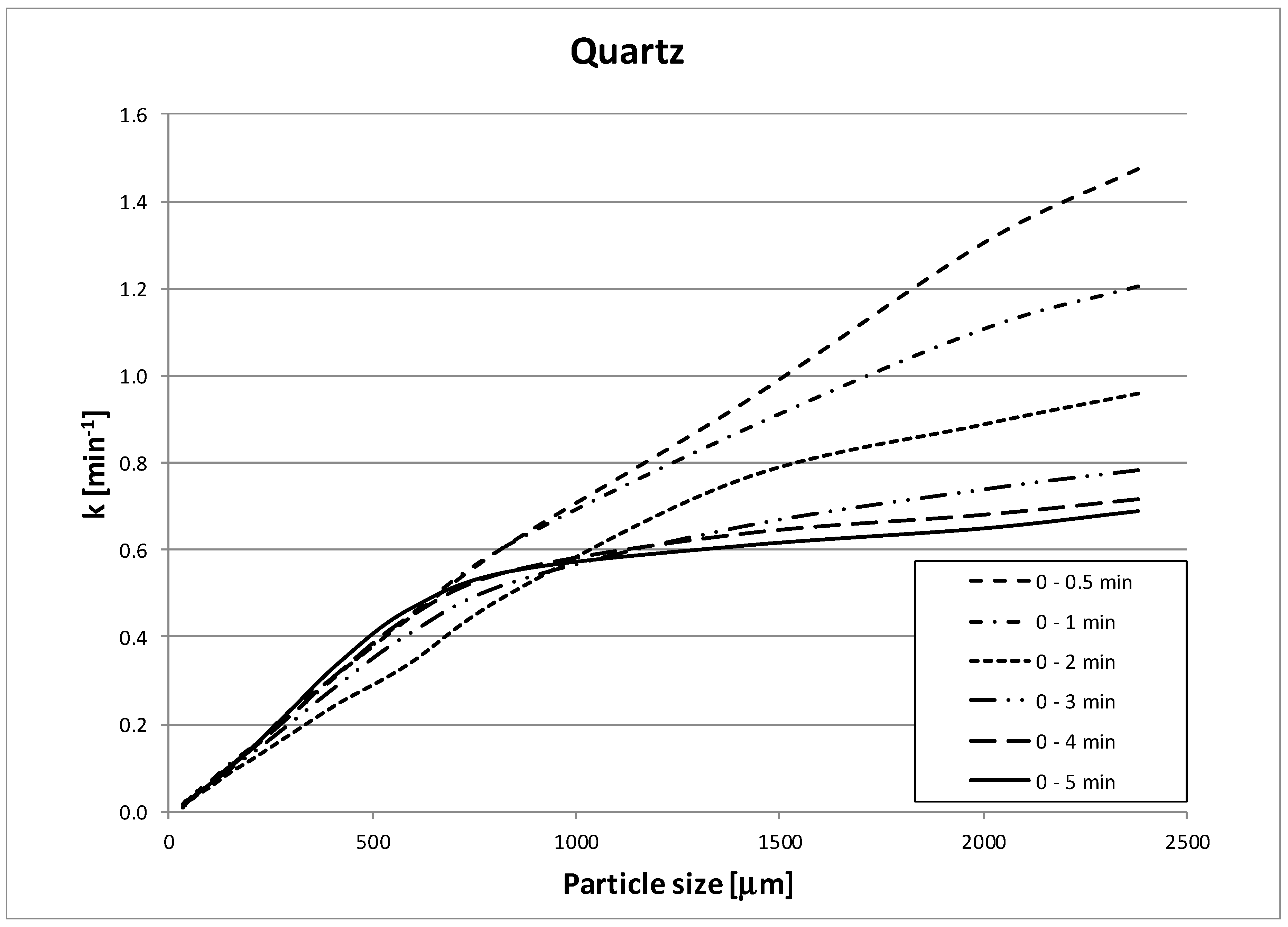
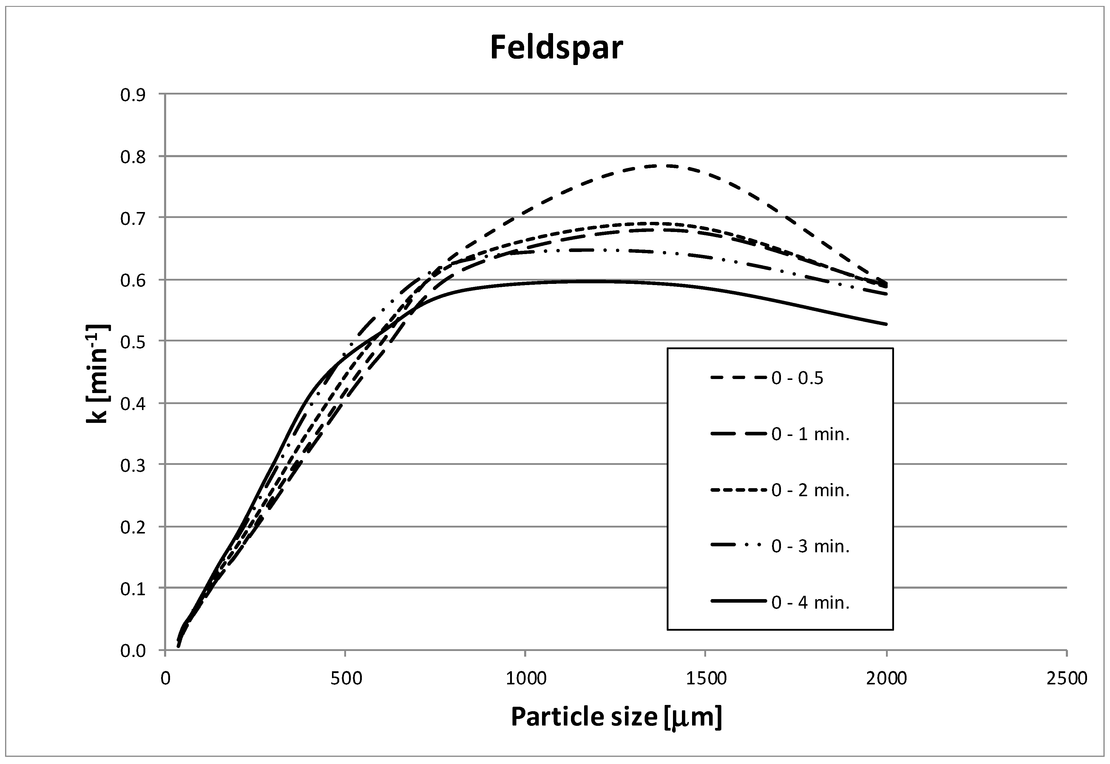
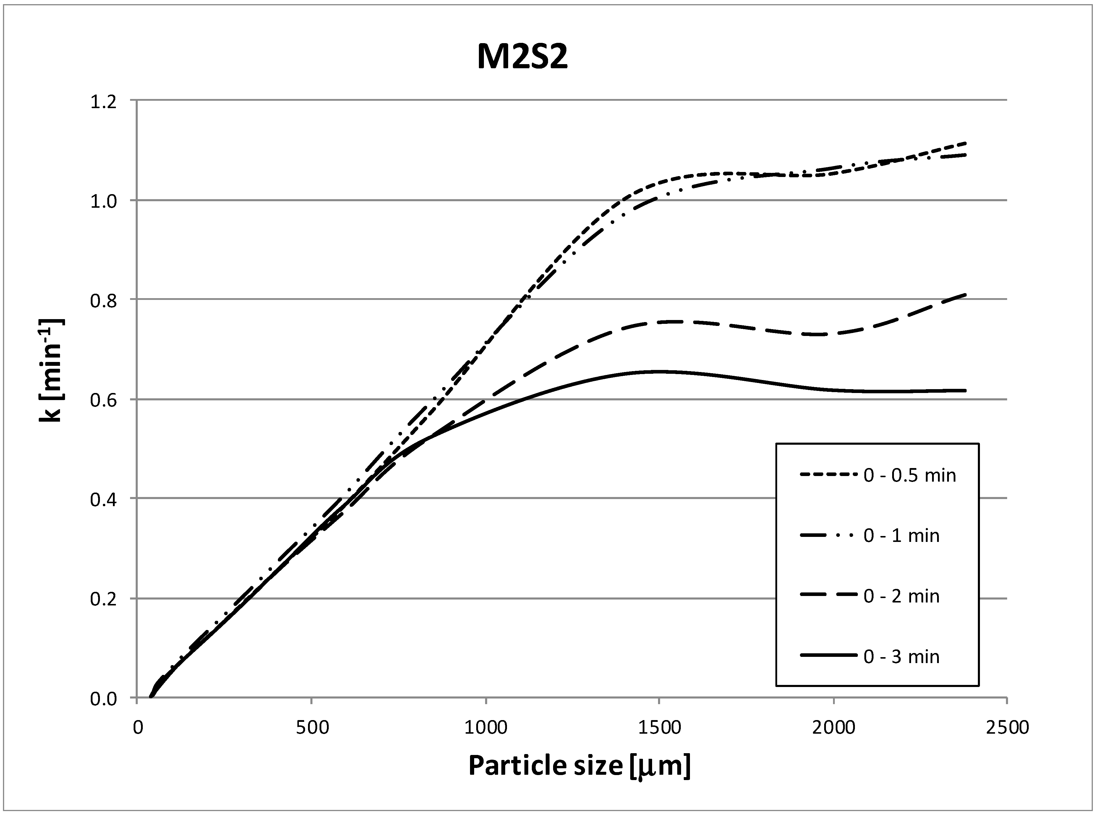
Determination of the slope (n) and the intercept on the y-axis (C) of the logarithmic-scale graph of k as a function of particle size (k vs. particle size).

Once the kinetic parameters are determined, the Bond test can be simulated, and the PSD can be obtained until reaching the grindability value (Gbp or grams per revolution) for a load of 250% and for the reference size (P₁₀₀). Once the feed characteristic grain size (F₈₀), the product characteristic grain size (P₈₀), and the grindability index (Gbp) are known, the Work Index can be calculated with Equation (6).

6. Conclusions

The experimental work done and its further analysis permit to draw the following conclusions:

• The conventional cumulative kinetic model (CKM) is a tool that allows determining the Work Index (w_i) for ball mill grinding, simulating the standard procedure of F.C. Bond. The respective results provided, according to literature, differ from less than 7%.
• A simplified procedure has been proposed to obtain the CKM parameters. It is based on determining k with one grinding time since k variation with particle size is rather constant for times less than 5 min. This makes it valid for simulating batch grinding with residence times on the order specified.
• The proposed simplified procedure has been proven to be valid for using the CKM to simulate the F.C. Bond’s standard test. It permits to obtain the Work Index in ball mill grinding for a reference size range between 840 (20 mesh) and 53 µm (400 mesh), yielding results that differ by less than 10% with respect to real values. This considerably reduces the involved laboratory work, thus being enough with one grinding run and two PSD determinations.

References

1. Rittinger von, P.R. Lehrbuch der Aufbereitungskunde; Ernst and Korn: Berlin, Germany, 1867. [Google Scholar]
2. Kick, F. Das Gesetz der Proportionalen Widerstände und Seine Anwendungen; Arthur Felix: Leipzig, Germany, 1885. [Google Scholar]
3. Bond, F.C. Third Theory of Comminution. Min. Eng. Trans. Aime 1952, 193, 484–494. [Google Scholar]
4. Bond, F.C. Crushing and Grinding Calculations; Allis Chalmers Manufacturing Co.: Milmwaukee, WI, USA, 1961. [Google Scholar]
5. Jankovic, A.; Dundar, H.; Mehta, R. Relationships between comminution energy and product size for a magnetite ore. J. South. Afr. Inst. Min. Metall. 2010, 110, 141–146. [Google Scholar]
6. Sepúlveda, J.; Gutierrez, R. Dimensionamiento y Optimización de Plantas Concentradoras Mediante Técnicas de Modelación Matemática; CIMM: Santiago, Chile, 1986. [Google Scholar]
7. Aksani, B.; Sönmez, B. Simulation of Bond Grindability Test by Using Cumulative Based Kinetic Model. Miner. Eng. 2000, 13, 673–677. [Google Scholar] [CrossRef]
8. Coello Velázquez, A.L.; Menéndez-Aguado, J.M.; Brown, R.L. Grindability of lateritic nickel ores in Cuba. Powder Technol. 2008, 182, 113–115. [Google Scholar] [CrossRef]
9. Berry, T.F.; Bruce, R.W. A simple method of determining the grindability of ores. Can. Min. J. 1966, 87, 63–65. [Google Scholar]
10. Menéndez-Aguado, J.M.; Dzioba, B.R.; Coello-Velazquez, A.L. Determination of work index in a common laboratory mill. Miner. Metall. Process. 2005, 22, 173–176. [Google Scholar] [CrossRef]
11. Bonoli, A.; Ciancabilla, F. The Ore Grindability Definition as an Energy Saving Tool in the Mineral Grinding Processes. In Proceedings of the 2nd International Congress “Energy, Environment and Technological Innovation”, Rome, Italy, 12–16 October 1992. [Google Scholar]
12. Chakrabarti, D.M. Simple Approach to Estimation of Work Index. Trans. Instn. Min. Met. Sect. C Min. Proc. Ext. Met. 2000, 109, 83–89. [Google Scholar] [CrossRef]
13. Napier- Munn, T.J.; Morrell, S.; Morrison, R.D.; Kojovic, T. Mineral Comminution Circuits: Their Operation and Optimization; JKMRC: Queensland, Australia, 1996. [Google Scholar]
14. Prediction of Bond’s work index from measurable rock properties. Int. J. Miner. Process. 2016, 157, 134–144.
15. Rodríguez, B.Á.; García, G.G.; Coello-Velázquez, A.L.; Menéndez-Aguado, J.M. Product size distribution function influence on interpolation calculations in the Bond ball mill grindability test. Int. J. Miner. Process. 2016, 157, 16–20. [Google Scholar] [CrossRef]
16. Lewis, K.A.; Pearl, M.; Tucker, P. Computer Simulation of the Bond Grindability Test. Miner. Eng. 1990, 3, 199–206. [Google Scholar] [CrossRef]
17. Silva, M.; Casali, A. Modelling SAG Milling Power and Specific Energy Consumption Including the Feed Percentage of Intermediate Size Particles. Miner. Eng. 2015, 70, 156–161. [Google Scholar] [CrossRef]
18. Menéndez-Aguado, J.M.; Coello-Velázquez, A.L.; Dzioba, B.R.; Diaz, M.A.R. Process models for simulation of Bond tests. Trans. Inst. Min. Metall. Sect. C Miner. Process. Extr. Metall. 2006, 115, 85–90. [Google Scholar] [CrossRef]
19. Lvov, V.V.; Chitalov, L.S. Comparison of the Different Ways of the Ball Bond Work Index Determining. Int. J. Mech. Eng. Technol. 2019, 10, 1180–1194. Available online: https://ssrn.com/abstract=3452642 (accessed on 5 June 2020).
20. Gharehgheshlagh, H.H. Kinetic grinding test approach to estimate the ball mill work index. Physicochem. Probl. Miner. Process. 2016, 52, 342–352. [Google Scholar]
21. Laplante, A.R.; Finch, J.A.; del Villar, R. Simplification of Grinding Equation for Plant Simulation. Trans. IMM Sec. C 1987, 96, C108–C112. [Google Scholar]
22. Loveday, B.K. An analysis of comminution kinetics in terms of size distribution parameters. J. S. Afr. Inst. Min. Metall. 1967, 68, 111–131. [Google Scholar]
23. Finch, J.A.; Ramirez-Castro, J. Modelling Mineral Size Reduction in Closed-Circuit Ball Mill at the Pine Point Mines Concentrator. Int. J. Min. Proc. 1981, 8, 67–78. [Google Scholar] [CrossRef]
24. Ersayin, S.; Sönmez, B.; Ergün, L.; Akasani, B.; Erkal, F. Simulation of the grinding circuit at Gümüşköy Silver Plant, Turkey. Trans. IMM Sect. C 1993, 102, C32–C38. [Google Scholar]
25. Ahmadi, R.; Shahsavari, S. Procedure for determination of ball Bond work index in the commercial operations. Miner. Eng. 2009, 22, 104–106. [Google Scholar] [CrossRef]
Figure 1. Determination of the kinetic constant, k, for a quartz sample; the lines are drawn from the starting point to the 5 min measurement.
Metals 10 00925 g001
Figure 2. Graph showing the variation of k with particle size for different grinding times, in the case of quartz.
Metals 10 00925 g002
Figure 3. Graph showing the variation of k with particle size for different grinding times, in the case of feldspar.
Metals 10 00925 g003
Figure 4. Graph showing the variation of k with particle size for different grinding times, in the case of M2S2 sample.
Metals 10 00925 g004