Abstract
The applicability of galvanic-cell-based atmospheric corrosion monitoring (ACM) technology has been confirmed empirically in field tests, however the corrosion behaviors on the ACM sensors have rarely been studied systematically. In this study, the influence of temperature, chloride ions, and hydrosulfite (simulated sulfur dioxide) ions on the corrosion behaviors of Fe/Cu-type ACM sensors was investigated. The results show that the hydrosulfite ions led to a larger increase in the Fe/Cu-based ACM current than chloride ions in the initial stage of corrosion, and both changed the components of the corrosion products. Moreover, the hydrosulfite and chloride ions showed a synergistic effect on the corroded ACM sensor. Lastly, a positive correlation between ACM technology and the mass loss method was observed, further indicating that ACM technology can be an effective, convenient, and fast approach to studying the accelerated corrosion behaviors of steels.
1. Introduction
Corrosion widely affects the infrastructure, transportation, and energy sectors [1,2,3,4], and atmospheric corrosion causes most of the loss and damage. At present, severity evaluations of atmospheric corrosion are mainly carried out by corrosion coupons [5,6,7], which are difficult to use to track the dynamic process of atmospheric corrosion continuously [8,9,10]. In contrast, atmospheric corrosion monitoring (ACM) technologies can create detailed descriptions of atmospheric corrosion, and help us to understand how such a process is influenced by the complex environmental parameters [11,12].
Various ACM technologies have been applied to assess the corrosivity of atmospheric environment based on different monitoring principles, such as the galvanic corrosion cell [13,14], electrochemical impedance [15,16,17], and electrical resistance [18,19] measurement. For galvanic-cell-based ACM sensors, active metals and noble metals are assembled as anodes and cathodes, respectively, in a closed cell to form galvanic couples, and a galvanometer is connected in series between the two kinds of electrodes to directly detect the galvanic current [13,14]. The corrosivity of the environment is reflected by the magnitude of the galvanic current, which is generated from the corroded sensor, instead of the substrate. Compared with the ACM technologies based on electrochemical impedance and electrical resistance measurements, the ACM with galvanic cells owns higher sensitivity to the change of atmospheric corrosivity, and avoids the interference of an external current that flows through the materials during measurement [15,16,18,19]. As a result, it is highly desirable to use the galvanic-cell-based ACM technology to assess the corrosivity and describe the corrosion performance of materials under atmospheric environments.
Different from the corrosion mechanism on corrosion coupons, the galvanic effect exists on the galvanic-cell-based ACM sensor. Empirically, the effectiveness of this sensor for sensitively measuring the dynamic changes of environmental corrosivity in the field has been verified [14,20,21,22]. Mansfeld et al. installed a Fe/Cu ACM sensor on the roof and observed that heavy fog significantly provoked the ACM current [20]. Pei et al. employed the Fe/Cu ACM sensor under six exposure fields and found that rain contributed to 64.6–89.0% of the corrosion of the steel, which only accounted for 16.3–29.7% of the exposure time [14]. Mizuno et al. and Pongsaksawad et al. obtained a positive correlation between the electrical quantity output of ACM sensors and the natural corrosion rate of corrosion coupons under three outdoor environments in Thailand and some automotive environments [21,22]. Furthermore, Pei et al. presented the application of machine learning methods to assist the analysis of ACM data and to predict the atmospheric corrosion [23]. However, few studies have evaluated the effectiveness in terms of corrosion products and morphologies. As a result, whether the galvanic effect changes the corrosion behaviors of the anodes on the ACM sensor is unknown. From the perspective of the corrosion behavior, the galvanic effect means the representation of the ACM sensors on standardized coupons can be doubtful. More detailed laboratory studies on the effectiveness of galvanic cell-based ACM technology and the scope of the applicable environments are urgently required.
In this study, an Fe/Cu-type ACM sensor was employed to study the corrosion behavior of steels on the ACM sensors under multiple types of simulated atmospheric environments, including atmospheres with no pollution, and atmospheres with chloride ions, sulfur dioxide, and both ionic contaminants, respectively. After testing, ACM technology was compared with the traditional mass loss method, and the correlation was discussed, with the aim of further verifying the reliability and feasibility of ACM technology for studying atmospheric corrosion in accelerated test environments.
2. Experimental Procedures
2.1. ACM Technology
A schematic diagram of the galvanic cell-based ACM technology is shown in Figure 1. The apparatus mainly consists of a sensor which generates the galvanic corrosion current, and a galvanometer (Saiyi IACM, Beijing, China) that detects the magnitude of the current. The ACM sensor comprises 11 corrosion couples, utilizing Q235 carbon steel (chemical composition given in Table 1) as the anodes and technical pure copper (>99.5% purity) as the cathodes. The anodes and cathodes are separated by glass fiber-reinforced epoxy composite boards (FR4) for electrical insulation. The FR4, with a thickness of 0.5 mm, is used to control the spacing between the metal sheets. The exposed area of each FR4 and metal electrode sheet is 25.0 mm × 0.5 mm. After being completely sealed, the surface of the sensor was abraded by 1200-grit sandpaper, and then we measured the resistance between the cathodes and anodes with a multimeter, making sure that they were not in short-circuit condition when the galvanometer was not connected. If the resistance was higher than 5 × 10⁶ Ohms, the ACM sensor was ready to use. The resolution of the monitored current was 0.01 μA, and the data acquisition frequency was set as once per minute. The measurement error of the galvanometer was within 0.5%.
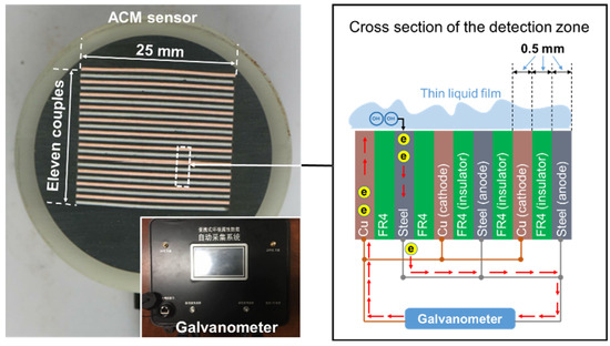
Figure 1.
Schematics showing the design of the Fe-Cu type atmospheric corrosion monitoring (ACM) sensor.

Table 1.
Chemical composition of the Q235 carbon steel (mass%)
When a thin layer of electrolyte is formed on the surface of the ACM sensor, the steels and coppers become electrically connected and this provokes a galvanic corrosion current. Due to the separation of the electrodes by the insulators, the galvanic current has to pass through a galvanometer, by which the ACM current was detected and recorded.
2.2. Laboratory Test Methods
The laboratory tests used to investigate the influence of different environmental factors on the ACM sensors were conducted in a salt spray box (Kemei-60 A), as shown in Figure 2. The size of the internal chamber of the salt spray box is 60 cm × 45 cm × 40 cm, and the pressure of compressed air is 1 ± 0.01 kgf cm−2, and the corrosive solution prepared for the spray is 15 L. Due to that it is difficult to keep the same condition at every location in the chamber, we installed the ACM sensor and the corrosion coupons at the same locations for each test, controlling the difference caused by different test locations. The deionized water (simulating the pure atmosphere), NaCl solution (simulating a marine environment with chloride), NaHSO3 solution (simulating an industrial environment with sulfur dioxide), and a mixed solution comprising NaCl and NaHSO3 were used as the corrosive mediums during the corrosion tests [24,25]. The detailed settings of the environmental factors for four in-door simulated atmospheric environments are shown in Table 2 [25]. To compare the obtained results of the ACM technology with those from the traditional mass loss method, five parallel Q235 carbon steel coupons (50 × 25 × 3 mm3) were placed in the same environment near the ACM sensor, so as to evaluate the atmospheric corrosivity by the mass loss rate.
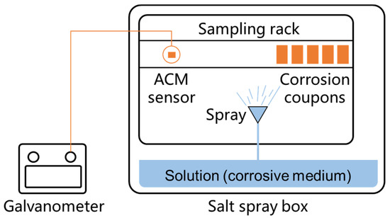
Figure 2.
Illustration of the spray test method in the laboratory.
Table 2.
Environmental factors used for the four simulated atmospheric environments in the laboratory
Each test lasted for 24 h. During testing, the real-time electrical outputs from the ACM sensor were acquired. When the tests were finished, the corrosion coupons were taken out, and the corrosion products on the carbon steel were removed by scrubbing with a wire brush in an 18 wt % hydrochloric acid solution, as specified in ISO8407 C.3.5 [26]. Then, the average mass loss was calculated using the weight difference of the specimens before and after the spray test.
2.3. Analytical Methods
After finishing the test, the macroscopic morphology of the ACM sensor surfaces was recorded by a Canon750D camera. The microstructure of the sensor surfaces was characterized by scanning electron microscopy (SEM, FEI Quanta250, Hillsboro, OR, USA), and all the SEM figures were shown as secondary electron images. Moreover, the crystal structures of the corrosion products on the Q235 metal sheets of ACM sensors were determined by X-ray diffracting (XRD, Rigaku Ultima IV, Tokyo, Japan) with CuKα radiation, and the scanning range was 10° to 90° in θ–2θ mode, with a scanning rate of 4°/min. The applied voltage was 40 kV and the filament current was 30 mA.
3. Results and Discussion
3.1. Effect of Temperature
Figure 3a displays the real-time values of the ACM current output from the ACM sensor under different temperatures. It is seen that the ACM current significantly increased after a certain time. This phenomenon can be explained by the working mechanism of the salt spray box. The salt spray box maintained its internal environment by intermittent spraying. When spraying, we observed a jump in the current values, showing that ACM technology could track and monitor the fluctuations of material corrosion caused by dynamic changes of environment. The macro morphologies of the sensor surface after 24-h spraying are shown in Figure 3b. Due to the weak corrosivity of deionized water and short corrosion time, the rust layers were thin and scattered over the surfaces of the sensors. As the temperature increased, the rust became more obvious. Combined with the ACM current variation in Figure 3a, the right peak of the ACM current caused by the second spray was obviously higher than that caused by the first spray for each temperature; this was caused by the promoting effect of the rust layer in forming a thicker thin liquid film during the initial stage of the corrosion [14]. The sensor surface was smooth for the first spray, but it was rusted during the second spray. Figure 3c shows the natural corrosion rate (r) acquired from the corrosion coupons and the average galvanic current (I) output by the ACM sensor under different temperatures during the continuous spray tests with deionized water. It can be clearly seen that both the corrosion rate and the average current increased with temperature. These results are in accordance with the laws in the Arrhenius equation [27,28,29], and the corrosion rate increased by nearly three times from 35 °C to 45 °C.
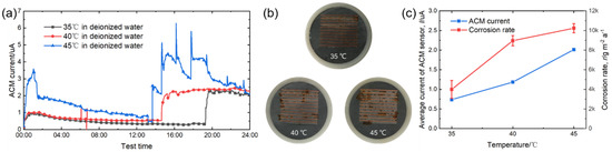
Figure 3.
(a) Real time ACM current; (b) the macro morphologies of the ACM sensor; (c) mass loss rate and average current of the ACM sensors at different temperatures.
The micro surface morphologies of the steels on the ACM sensors after testing with deionized water are shown in Figure 4. The corrosion products were granular and stacked, with high porosity and poor protection to the substrate. These corrosion products could not inhibit the oxygen transmission, but were more conducive to the formation of a thin liquid film, and caused the ACM current to have an increasing trend in Figure 3a. Figure 5 shows the XRD results of the corrosion products at different temperatures. The compositions of these corrosion products were all mainly magnetite (Fe3O4), with a small amount of lepidocrocite (γ-FeOOH) and goethite (α-FeOOH). As a result, higher temperatures only accelerated the corrosion process but did not vary the corrosion behaviors on the Fe/Cu-based ACM sensor.
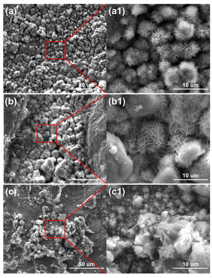
Figure 4.
Surface morphology of the corrosion products formed on the anodes of the ACM sensor after the continuous spray test with deionized water at different temperatures: (a) 35 °C; (b) 40 °C; (c) 45 °C.
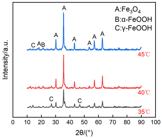
Figure 5.
Composition of the corrosion products formed on the anodes of the ACM sensor after the continuous spray test with deionized water at different temperatures.
3.2. Effect of Chlorine Ions
Figure 6a demonstrates the real-time variation of the ACM current under different concentrations of NaCl solutions. Compared with deionized water, chloride ions in NaCl solution caused the evaporation process of the thin liquid film to become more difficult and did not show the same promoting effect for the second spray. After 24 h, the ACM current under 3.5% NaCl showed the highest value. The surfaces of the corroded ACM sensors are shown in Figure 6b; the corrosion was slight, and the macro morphology did not alter significantly with the changed NaCl concentrations. Figure 6c shows the natural corrosion rate data and average ACM galvanic current data under different NaCl solution concentrations. Obviously, the average current of the ACM sensor increased significantly when we used 1% NaCl solution as the corrosion medium instead of deionized water. Then, the concentration of NaCl solution changed from 1% to 7% and the average current became constant. The influence of chloride on material corrosion was dominant due to the hygroscopicity, penetrability, and electroconductibility [30], and the concentration directly affected the corrosion rate in yearly field tests [30,31,32,33]. These promoting effects lead to a higher average current of the ACM sensor from 0% to 1% concentration, as shown in Figure 6c. However, the crucial mechanism of chloride in promoting corrosion is accumulation in the rust layers, inducing the formation of non-protective corrosion products [30,32,34,35]. This leads to the impact of chloride being cumulative, and it becomes more dominant in long-term tests under marine atmospheres. For example, Alcántara et al. found that for the first half year of atmospheric corrosion, the corrosion rates of mild steel were 118.6 μm a−1 and 114 μm a−1 in the locations with chloride deposition rates of ~100 mg m−2 d−1 and ~50 mg m−2 d−1, respectively. After one year, the corrosion rates exhibited a larger difference (65.5 μm a−1 and 50.1 μm a−1) [32]. For the tests in this study, the corrosion time was short, and the corrosion stage was speculated to be in the initial stage. Therefore, it is reasonable to consider the promoting effect of chloride with different NaCl concentrations (1–7%) was not obvious in this study, which leads to similar macro morphologies and average ACM currents, as seen in Figure 6b,c. Moreover, we observed the highest value under 3.5% NaCl solution, both in average ACM current and corrosion rate. This phenomenon might be attributed to the strong electrolytes. According to the theory of strong electrolytes, the migrating rates of the ions should slow down owing to the increasing interaction of Na+ and chloride ions with a high concentration of NaCl solution, which does not favor increasing the conductivity of the electrolyte film and slightly inhibits corrosion [36]. The increase in ions also reduced the dissolved oxygen [37]. As a result, a decline in both the current and corrosion rate was observed above a NaCl concentration of 3.5%, as shown in Figure 6c. Furthermore, the natural corrosion rate of the steels and ACM current had a similar development trend.
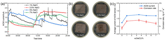
Figure 6.
(a) Real time ACM current; (b) the macro morphologies of the ACM sensor; (c) mass loss rate and average current of the ACM sensor at different concentrations of NaCl solution.
The micro morphologies of the steels on the ACM sensor during the NaCl spray are shown in Figure 7. The morphologies at each concentration were similar, all illustrating large plate-like particles with high porosity and big gaps, which are the typical features of lepidocrocite. The corrosion products were speculated to be non-protective due to their structure. That assumption was verified by the XRD results in Figure 8, showing that the compositions of these corrosion products were the same, indicating the change in the NaCl concentration did not vary the composition of corrosion products formed on the surface of the ACM sensor. The corrosion products were mainly lepidocrocite, with a small amount of goethite and magnetite, which were different from the corrosion products under deionized water. The difference might be attributed to the presence of chloride ions. Previous studies showed that chloride ions would be benefit to form more lepidocrocite in the rust layers at first, and then akaganeite (β-FeOOH) as time went on [30,38]. This caused the same corrosion behavior on the sensor: lepidocrocite became the main component in the rust layers, as shown in Figure 8. The porous structure and strong electrochemical activity of lepidocrocite would further enhance the moisture absorption and provoke a higher ACM current on the sensor, similar to the increase in the corrosion rate of the coupons. In summary, the corrosion behaviors of the ACM sensor were in accordance with that of the coupons under an environment with chlorine ions.
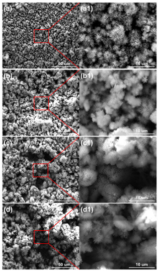
Figure 7.
Surface morphology of the corrosion products formed on the anodes of the ACM sensor after the continuous spray test with NaCl solution at different concentrations: (a) 1%; (b) 3.5%; (c) 5%; (d) 7%.
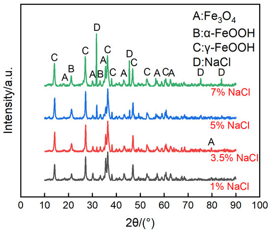
Figure 8.
Composition of corrosion products formed on the anodes of the ACM sensor after the continuous spray test with NaCl solution at different concentrations.
3.3. Effect of Hydrosulfite Ions
Figure 9a shows the real-time ACM current data under different concentrations of NaHSO3 solution. Compared with Figure 3a and Figure 6a, the current values observed here were larger due to the introduction of acidic ions. The current showed a downward trend in sulfate solutions during 24-h spray. The macro morphologies in Figure 9b show that the corrosion products covered the surface on the ACM sensors, and the corrosion tended to be more severe with increased acidic ions. The developing trend of the natural corrosion rate and average galvanic current was similar, as shown in Figure 9c. Unlike chloride ions, hydrosulfite ions not only enhanced the conductivity of the electrolyte layer, but also provided an anodic depolarizer. Thus, the hydrosulfite ions were more corrosive at the initial stage of corrosion than chloride ions [39,40]. Furthermore, this environment triggered an excessive galvanic effect, and led to an obviously higher current and corrosion rate when the concentration of hydrosulfite ions rose, as shown in Figure 9c.
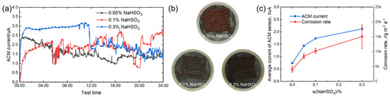
Figure 9.
(a) Real time ACM current; (b) the macro morphologies of the ACM sensor; (c) the variation of the mass loss rate and average current of the ACM sensor at different concentrations of NaHSO3 solution.
Figure 10 shows the surface morphologies of the steel on the ACM sensors after spraying with NaHSO3 solution. It was observed that the block structure morphology became increasingly prevalent as the NaHSO3 concentration increased from 0.05% to 0.3%. Usually, hydrosulfite ions lower the pH of electrolytes and dissolve the initial corrosion products of lepidocrocite [41], which causes lepidocrocite to exist in the outer rust layer. Here, higher concentrations of hydrosulfite ions resulted in more goethite and iron hydrosulfite (FeSO3) and caused denser microtopography with some cracks of the corrosion products, as shown in Figure 10c. As for the cracks on the inner layer, the growth of goethite and iron hydrosulfite resulted in stress on the interface between the rust layer and substrate. Due to the poor deformation capacity of the rust, cracks were generated in the inner rust layer. As mentioned above, the current showed a downward trend in sulfate solutions (Figure 9a), and we speculated that an environment with higher corrosivity made the corrosion process faster in the initial stage. Then, the ACM current showed a declining trend over a short time. Besides, the corrosion products seemed to be more protective in the sulfate solutions, which would inhibit the contact between the corrosive medium and substrate. Both of these may have caused the downward trend in the sulfate solutions. The XRD results are shown in Figure 11. The main corrosion products were lepidocrocite under 0.05% NaHSO3 solution. When the concentration of solution reached 0.3%, the content of lepidocrocite and goethite decreased, and iron hydrosulfite could be detected easily, which verified the speculations above. The unchanged type of corrosion products signified the change in the NaHSO3 concentration did not influence the corrosion mechanism of the anodes on the ACM sensor. However, the primary component of the corrosion products changed from lepidocrocite to iron hydrosulfite, showing the dominant change of corrosion process into the depolarization of the acid ions. This XRD result and the micro morphology of the corrosion products were similar to those found in a previous study investigating corrosion coupons [42], indicating that the corrosion behaviors under similar environments were consistent.
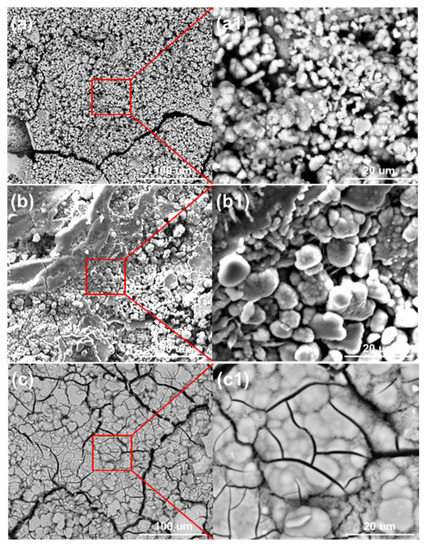
Figure 10.
Surface morphology of corrosion products formed on the anodes of the ACM sensor after the continuous spray tests at different concentrations of NaHSO3 solution: (a) 0.05%; (b) 0.1%; (c) 0.3%.
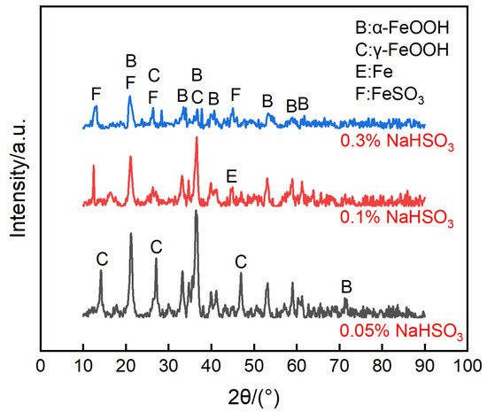
Figure 11.
Composition of the corrosion products formed on the anodes of the ACM sensor after the continuous spray tests at different concentrations of NaHSO3 solution.
3.4. Effect of Combined Ionic Contaminants
Figure 12 shows the real-time ACM current data, the macro morphologies of the ACM sensors, the natural corrosion rate curve, and the average ACM galvanic current curve under different concentrations of NaCl with 0.1% NaHSO3. Compared with Figure 6, the corrosion became more serious with the addition of 0.1% NaHSO3. Moreover, as seen in Figure 12c, the presence of an additional 3.5% NaCl was of benefit for raising the ACM current and corrosion rate in the 0.1% NaHSO3 solution, showing that the promoting effect of chloride was not inhibited by the addition of NaHSO3. In summary, the combined effect of chloride and hydrosulfite ions on the corrosion of steels, both in the ACM sensors and in the corrosion coupons, was greater than that caused by each single component.
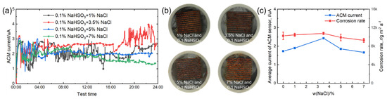
Figure 12.
(a) Real time ACM current, (b) the macro morphologies of the ACM sensor; (c) the variation of mass loss rate and average current of ACM sensor at 0.1% NaHSO3 concentration with different concentrations of NaCl solution.
As shown in Figure 13, the morphologies of the corrosion products on the sensors were complex. Filamentous products floated on the surface, and small-sized blocks with many cracks sank to the bottom. The corrosion products were mainly goethite and iron hydrosulfite, with less lepidocrocite, which was demonstrated by the XRD results in Figure 14. We speculate that the chloride ions could not significantly improve the ACM current in the acidic environment due to the partial dissolution of the lepidocrocite. This speculated corrosion behavior is similar to the synergistic effect of chloride ions and sulfur dioxide on the coupons [43,44].
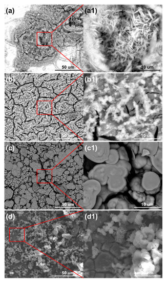
Figure 13.
Surface morphology of corrosion products formed on the anodes of the ACM sensor after the continuous spray tests of mixed solution at 0.1% NaHSO3 concentration, with different concentrations of NaCl solution: (a) 1%; (b) 3.5%; (c) 5%; (d) 7%.
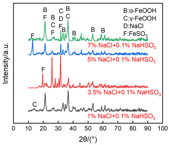
Figure 14.
Composition of corrosion products formed on the anodes of the ACM sensor after the continuous spray tests of mixed solution at 0.1% NaHSO3 concentration, and different concentrations of NaCl solution.
3.5. Correlation between the ACM Current and Corrosion Rate
Figure 15 presents the correlation between the average current of the ACM sensor (I) and corrosion rate of the corrosion coupons (r). The correlation equation is written as
where r is expressed in g m−2 a−1 and I is expressed in μA. As seen in Figure 9b and Figure 12b, the corrosion products covered the surface of the sensors. We considered that the conductivity of the corrosion products might cause a short-circuit of the ACM sensors, leading to a rapid decrease in the detected current. Nevertheless, despite the different environments, I correlated well with r, indicating the negligible influence of the short circuit. Among the corrosion products (e.g., magnetite, goethite, lepidocrocite, and ferrihydrite), magnetite has the highest conductivity [45]. However, Figure 9b and Figure 12b show that the main corrosion products formed after the test were goethite, lepidocrocite, and iron hydrosulfite, without magnetite. More importantly, the electrical resistivity of the electrolyte layer (0.5–5 Ohms cm [46,47]) formed on the sensor surface was expected to be much lower than that of the corrosion product oxide layers on the steel surfaces (106–1.1 × 10⁸ Ohms cm) [48]. Thus, we inferred that the change in the corrosion product conductivity would not induce a major impact on the sensor output current. In this way, a good correlation between the average current of the ACM sensor and the corrosion rate of the corrosion coupons was achieved.
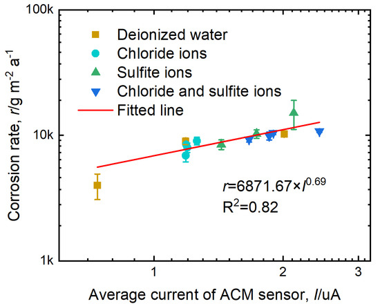
Figure 15.
Relationship between the average current of the ACM sensor and corrosion rate of the corrosion coupons.
4. Conclusions
A Fe/Cu-type ACM sensor was employed to explore the influence of different environmental factors on the ACM sensor, and investigate the corrosion behaviors of the steels on the ACM sensor. A higher temperature only accelerated the corrosion process of the ACM sensor, but did not alter the corrosion behaviors. The chloride ions promoted the formation of lepidocrocite in the rust layers on the ACM sensor surface and increased the current values. Meanwhile, the hydrosulfite ions led to a larger increase in the ACM current than chloride ions at the initial stage of corrosion, and changed the components and morphologies of the corrosion products, especially under a high concentration of hydrosulfite ions. Moreover, the hydrosulfite and chloride ions exhibited a synergistic effect on the corroded ACM sensor. The investigated corrosion behaviors under multiple environments on the ACM sensor surface were in accordance with the corrosion coupons. Lastly, a positive correlation between the ACM technology and the mass loss method was observed, and we found that the coverage of the corrosion products did not affect the effectiveness of the sensor in this study. In summary, from the perspective of corrosion behaviors, the representation of the ACM sensors regarding the standardized coupons was feasible. ACM technology can be an effective, convenient, and fast approach to study the accelerated corrosion behaviors of steels.
Our future work will focus on quantitatively establishing a transformational correlation between the real-time ACM current and the instantaneous corrosion rate, considering changes in environmental factors and an extended timeframe. It is expected that this approach would expand the usefulness of ACM technology for the evaluation of the corrosion resistance of materials.
Author Contributions
Conceptualization, K.X. and X.L.; Methodology, Z.P. and L.C.; Formal analysis, Z.P.; Investigation, Z.P., Q.L., and J.W.; Data curation, L.C.; Writing—original draft preparation, Z.P.; Writing—review and editing, Z.P., K.X., L.M., and X.L.; Supervision, K.X. and X.L.; Project administration, X.L. All authors have read and agreed to the published version of the manuscript.
Funding
This research was funded by the National Key Research and Development Program of China (no. 2016YFB0700500).
Acknowledgments
The authors acknowledge financial support from the National Key Research and Development Program of China (no. 2016YFB0700500) and National Environmental Corrosion Platform.
Conflicts of Interest
The authors declare no conflict of interest.
References
- Li, X.; Zhang, D.; Liu, Z.; Li, Z.; Du, C.; Dong, C. Materials science: Share corrosion data. Nature 2015, 527, 441–442. [Google Scholar] [CrossRef] [PubMed]
- Grøntoft, T.; Verney-Carron, A.; Tidblad, J. Cleaning costs for European sheltered white painted steel and modern glass surfaces due to air pollution since the year 2000. Atmosphere 2019, 10, 167. [Google Scholar] [CrossRef]
- Javaherdashti, R. How corrosion affects industry and life. Anti-Corros. Methods Mater. 2000, 47, 30–34. [Google Scholar] [CrossRef]
- Shi, Y.; Yang, B.; Liaw, P.K. Corrosion-Resistant High-Entropy Alloys: A Review. Metals 2017, 7, 43. [Google Scholar] [CrossRef]
- Azmat, N.S.; Ralston, K.D.; Muddle, B.C.; Cole, I.S. Corrosion of Zn under acidified marine droplets. Corros. Sci. 2011, 53, 1604–1615. [Google Scholar] [CrossRef]
- Thierry, D.; LeBozec, N. Corrosion products formed on confined hot-dip galvanized steel in accelerated cyclic corrosion tests. Corrosion 2009, 65, 718–725. [Google Scholar] [CrossRef]
- Veleva, L.; Pérez, G.; Acosta, M. Statistical analysis of the temperature-humidity complex and time of wetness of a tropical climate in the Yucatan Peninsula in Mexico. Atmos. Environ. 1997, 31, 773–776. [Google Scholar] [CrossRef]
- Boelen, B.; Schmitz, B.; Defourny, J.; Blekkenhorst, F. A literature survey on the development of an accelerated laboratory test method for atmospheric corrosion of precoated steel products. Corros. Sci. 1993, 34, 1923–1931. [Google Scholar] [CrossRef]
- Institute, T.B.S. Corrosion of metals and alloys—Corrosivity of atmospheres—Classification, determination and estimation. In ISO 9223: 2012; The British Standard Institute: London, UK; European Committee for Standardization: Brussels, Belgium, 2012. [Google Scholar]
- Zhi, Y.; Fu, D.; Zhang, D.; Yang, T.; Li, X. Prediction and Knowledge Mining of Outdoor Atmospheric Corrosion Rates of Low Alloy Steels Based on the Random Forests Approach. Metals 2019, 9, 383. [Google Scholar] [CrossRef]
- Purwasih, N.; Kasai, N.; Okazaki, S.; Kihira, H. Development of Amplifier Circuit by Active-Dummy Method for Atmospheric Corrosion Monitoring in Steel Based on Strain Measurement. Metals 2018, 8, 5. [Google Scholar] [CrossRef]
- Purwasih, N.; Kasai, N.; Okazaki, S.; Kihira, H.; Kuriyama, Y. Atmospheric Corrosion Sensor Based on Strain Measurement with an Active Dummy Circuit Method in Experiment with Corrosion Products. Metals 2019, 9, 579. [Google Scholar] [CrossRef]
- Shi, Y.; Fu, D.; Zhou, X.; Yang, T.; Zhi, Y.; Pei, Z.; Zhang, D.; Shao, L. Data mining to online galvanic current of zinc/copper Internet atmospheric corrosion monitor. Corros. Sci. 2018, 133, 443–450. [Google Scholar] [CrossRef]
- Pei, Z.; Cheng, X.; Yang, X.; Li, Q.; Xia, C.; Zhang, D.; Li, X. Understanding environmental impacts on initial atmospheric corrosion based on corrosion monitoring sensors. J. Mater. Sci. Technol. 2020. [Google Scholar] [CrossRef]
- Nishikata, A.; Zhu, Q.; Tada, E. Long-term monitoring of atmospheric corrosion at weathering steel bridges by an electrochemical impedance method. Corros. Sci. 2014, 87, 80–88. [Google Scholar] [CrossRef]
- Yadav, A.P.; Suzuki, F.; Nishikata, A.; Tsuru, T. Investigation of atmospheric corrosion of Zn using ac impedance and differential pressure meter. Electrochim. Acta 2004, 49, 2725–2729. [Google Scholar] [CrossRef]
- Thee, C.; Hao, L.; Dong, J.; Mu, X.; Wei, X.; Li, X.; Ke, W. Atmospheric corrosion monitoring of a weathering steel under an electrolyte film in cyclic wet–dry condition. Corros. Sci. 2014, 78, 130–137. [Google Scholar] [CrossRef]
- Kamsu-Foguem, B. Knowledge-based support in Non-Destructive Testing for health monitoring of aircraft structures. Adv. Eng. Inform. 2012, 26, 859–869. [Google Scholar] [CrossRef]
- Li, Z.; Fu, D.; Li, Y.; Wang, G.; Meng, J.; Zhang, D.; Yang, Z.; Ding, G.; Zhao, J. Application of An Electrical Resistance Sensor-Based Automated Corrosion Monitor in the Study of Atmospheric Corrosion. Materials 2019, 12, 1065. [Google Scholar] [CrossRef] [PubMed]
- Mansfeld, F.; Kenkel, J.V. Electrochemical monitoring of atmospheric corrosion phenomena. Corros. Sci. 1976, 16, 111–122. [Google Scholar] [CrossRef]
- Mizuno, D.; Suzuki, S.; Fujita, S.; Hara, N. Corrosion monitoring and materials selection for automotive environments by using Atmospheric Corrosion Monitor (ACM) sensor. Corros. Sci. 2014, 83, 217–225. [Google Scholar] [CrossRef]
- Pongsaksawad, W.; Viyanit, E.; Sorachot, S.; Shinohara, T. Corrosion assessment of carbon steel in Thailand by atmospheric corrosion monitoring (ACM) sensors. J. Met. Mater. Miner. 2010, 20, 23–27. [Google Scholar]
- Pei, Z.; Zhang, D.; Zhi, Y.; Yang, T.; Jin, L.; Fu, D.; Cheng, X.; Terryn, H.A.; Mol, J.M.C.; Li, X. Towards understanding and prediction of atmospheric corrosion of an Fe/Cu corrosion sensor via machine learning. Corros. Sci. 2020, 170, 108697. [Google Scholar] [CrossRef]
- Liu, Q.; Luo, H.; Dong, C.F.; Xiao, K.; Li, X.G. The electrochemical behavior of brass in NaHSO3 solution without and with Cl. Int. J. Electrochem. Sci. 2012, 7, 11123–11136. [Google Scholar]
- Cheng, X.; Jin, Z.; Liu, M.; Li, X. Optimizing the nickel content in weathering steels to enhance their corrosion resistance in acidic atmospheres. Corros. Sci. 2017, 115, 135–142. [Google Scholar] [CrossRef]
- Qian, H.; Zhang, D.; Lou, Y.; Li, Z.; Xu, D.; Du, C.; Li, X. Laboratory investigation of microbiologically influenced corrosion of Q235 carbon steel by halophilic archaea Natronorubrum tibetense. Corros. Sci. 2018, 145, 151–161. [Google Scholar] [CrossRef]
- Qiu, L.-G.; Wu, Y.; Wang, Y.-M.; Jiang, X. Synergistic effect between cationic gemini surfactant and chloride ion for the corrosion inhibition of steel in sulphuric acid. Corros. Sci. 2008, 50, 576–582. [Google Scholar] [CrossRef]
- Soltis, J.; Laycock, N.J.; Krouse, D. Temperature dependence of the pitting potential of high purity aluminium in chloride containing solutions. Corros. Sci. 2011, 53, 7–10. [Google Scholar] [CrossRef]
- Prosek, T.; Nazarov, A.; Stoulil, J.; Thierry, D. Evaluation of the tendency of coil-coated materials to blistering: Field exposure, accelerated tests and electrochemical measurements. Corros. Sci. 2012, 61, 92–100. [Google Scholar] [CrossRef]
- Ma, Y.; Li, Y.; Wang, F. Corrosion of low carbon steel in atmospheric environments of different chloride content. Corros. Sci. 2009, 51, 997–1006. [Google Scholar] [CrossRef]
- Morcillo, M.; Chico, B.; Díaz, I.; Cano, H.; Fuente, D.D.L. Atmospheric corrosion data of weathering steels. A review. Corros. Sci. 2013, 77, 6–24. [Google Scholar] [CrossRef]
- Alcántara, J.; Chico, B.; Díaz, I.; Fuente, D.D.L.; Morcillo, M. Airborne chloride deposit and its effect on marine atmospheric corrosion of mild steel. Corros. Sci. 2015, 97, 74–88. [Google Scholar]
- Krivy, V.; Kubzova, M.; Kreislova, K.; Urban, V. Characterization of Corrosion Products on Weathering Steel Bridges Influenced by Chloride Deposition. Metals 2017, 7, 336. [Google Scholar] [CrossRef]
- Mi, N.; Ghahari, M.; Rayment, T.; Davenport, A.J. Use of inkjet printing to deposit magnesium chloride salt patterns for investigation of atmospheric corrosion of 304 stainless steel. Corros. Sci. 2011, 53, 3114–3121. [Google Scholar] [CrossRef]
- Weissenrieder, J.; Leygraf, C. In situ studies of filiform corrosion of iron. J. Electrochem. Soc. 2004, 151, B165–B171. [Google Scholar] [CrossRef]
- Qu, Q.; Yan, C.W.; Zhang, L.; Wan, Y.; Cao, C.N. Influence of Nacl Deposition on Atmospheric Corrosion of A3 Steel in the Presence of SO2. Acta Metall. Sin. Engl. Lett. 2002, 15, 409–415. [Google Scholar]
- Liu, S.; Sun, H.; Sun, L.; Fan, H. Effects of pH and Cl− concentration on corrosion behavior of the galvanized steel in simulated rust layer solution. Corros. Sci. 2012, 65, 520–527. [Google Scholar] [CrossRef]
- Sudakar, C.; Subbanna, G.N.; Kutty, T.R.N. Effect of anions on the phase stability of γ-FeOOH nanoparticles and the magnetic properties of gamma-ferric oxide derived from lepidocrocite. J. Phys. Chem. Solids 2003, 64, 2337–2349. [Google Scholar] [CrossRef]
- Wang, Z.; Liu, J.; Wu, L.; Han, R.; Sun, Y. Study of the corrosion behavior of weathering steels in atmospheric environments. Corros. Sci. 2013, 67, 1–10. [Google Scholar] [CrossRef]
- Okonkwo, P.C.; Shakoor, R.A.; Benamor, A.; Mohamed, A.M.A.; Al-Marri, M.J.F.A. Corrosion Behavior of API X100 Steel Material in a Hydrogen Sulfide Environment. Metals 2017, 7, 109. [Google Scholar] [CrossRef]
- Wang, J.H.; Wei, F.I.; Chang, Y.; Shih, H.C. The corrosion mechanisms of carbon steel and weathering steel in SO2 polluted atmospheres. Mater. Chem. Phys. 1997, 47, 1–8. [Google Scholar] [CrossRef]
- Misawa, T.; Asami, K.; Hashimoto, K.; Shimodaira, S. The mechanism of atmospheric rusting and the protective amorphous rust on low alloy steel. Corros. Sci. 1974, 14, 279–289. [Google Scholar] [CrossRef]
- Cao, X.; Xu, C. Synergistic effect of chloride and sulfite ions on the atmospheric corrosion of bronze. Mater. Corros. 2006, 57, 400–406. [Google Scholar] [CrossRef]
- Knotkova, D.; Dean, S.W.; Kreislova, K. International Atmospheric Exposure Program: Summary of Results: Developed by ISO/TC 156/WG 4, Atmospheric Corrosion Testing and Classification of Corrosivity of Atmosphere; ASTM International: West Conshohocken, PA, USA, 2010; pp. 10–65. [Google Scholar]
- Guskos, N.; Papadopoulos, G.J.; Likodimos, V.; Patapis, S.; Yarmis, D.; Przepiera, A.; Przepiera, K.; Majszczyk, J.; Typek, J.; Wabia, M.; et al. Photoacoustic, EPR and electrical conductivity investigations of three synthetic mineral pigments: Hematite, goethite and magnetite. Mater. Res. Bull. 2002, 37, 1051–1061. [Google Scholar] [CrossRef]
- Jagannadha Sarma, V.V.; Subba Rao, C. Electrical conductivity of rain water at Visakhapatnam, India. J. Geophys. Res. 1972, 77, 2197–2200. [Google Scholar] [CrossRef]
- Hermans, T.; Paepen, M. Combined Inversion of Land and Marine Electrical Resistivity Tomography for Submarine Groundwater Discharge and Saltwater Intrusion Characterization. Geophys. Res. Lett. 2020, 47, e2019GL085877. [Google Scholar] [CrossRef]
- Habib, K. Measurement of surface resistivity/conductivity of carbon steel in 5–20 ppm of KGR-134 inhibited seawater by holographic interferometry techniques. In Optical Measurement Systems for Industrial Inspection VII, Proceedings of the SPIE—International Society for Optics and Photonics, Munich, Germany, 23–26 May 2011; Peter, L., Ed.; Curran Associates: Manila, Philippines, 2011. [Google Scholar]


© 2020 by the authors. Licensee MDPI, Basel, Switzerland. This article is an open access article distributed under the terms and conditions of the Creative Commons Attribution (CC BY) license (http://creativecommons.org/licenses/by/4.0/).