Article

Environmental Fatigue Analysis of Nuclear Structural Components: Assessment Procedures, Loads, and a Case Study

1
LADICIM (Laboratory of Materials Science and Engineering), University of Cantabria, E.T.S. de Ingenieros de Caminos, Canales y Puertos, Av/ Los Castros 44, Santander, 39005 Cantabria, Spain
2
EDF China, Beijing 100000, China
3
INESCO Ingenieros, CDTUC, Av/ Los Castros 44, Santander, 39005 Cantabria, Spain
4
EDF – DIPNN – DT, 69001 Lyon, France
*
Author to whom correspondence should be addressed.
Metals 2020, 10(5), 609; https://doi.org/10.3390/met10050609
Submission received: 20 April 2020 / Revised: 6 May 2020 / Accepted: 7 May 2020 / Published: 8 May 2020
(This article belongs to the Special Issue Environmental Fatigue Assessment of Metallic Materials and Components)

Abstract

:
Nowadays, environmental fatigue assessment is mandatory in many countries, in the design and operational stages of nuclear structural components. The analysis of environmental fatigue can be a complex engineering process that is generally performed following national or international procedures. Such procedures are not always based on the same assumptions, and novel analysts may find a confusing variety of documents. Moreover, once a specific procedure has been chosen for the analysis, it is possible to complete the fatigue assessment by using design transients (and loads) or, alternatively, real loads provided by monitoring systems. In this context, this paper provides a comprehensive review of the different environmental fatigue assessment procedures and a brief description of the different types of load inputs (design vs. real data). The work is completed with a case study, in which the (fatigue) cumulative usage factor is estimated in a particular nuclear component by using one of the abovementioned assessment procedures (NUREG/CR-6909) and two options for the load inputs.

1. Introduction

Fatigue is an important degradation mechanism for pressure vessels and piping systems, especially in nuclear power plants (NPPs). Consequently, a great deal of scientific work has been undertaken and numerous tests have been performed to understand the principles and find rules to deal with this issue [1]. Fatigue evaluation plays a significant role in assuring the integrity of aged plant components. The fact that the fatigue life may be reduced in (nuclear) aggressive environments was first discovered in Japan in the 1980’s and in the last four decades, this situation has been widely studied in NPPs [2].
However, experimental results have indicated that additional parameters should be taken into account to describe the influence of the coolant on the fatigue performance of pressure vessels and piping systems of light water reactors (LWRs) [1]. Different laboratory works have identified the influence of key parameters on fatigue cracking and have established the effects of these key parameters on the fatigue life of selected steels used in nuclear plants [3,4]. These key parameters are the strain rate, the fluid/metal temperature, and the concentration of dissolved oxygen (DO) in the water. Other parameters, such as water flow or thermal treatment, also have some influence, while the sulphur content also has an influence in carbon and low alloy steels.
Nevertheless, it is also known that there are other parameters affecting the fatigue life, such as the surface roughness [5,6], mean stress [5,6], and existence of hold periods in the strain waveform [7,8], which are not directly considered in the fatigue design of NPP components. The effect of these parameters is implicitly considered in safety factors or design curves, but their precise effect is not well-known and great benefits (e.g., better designs and higher safety) could be obtained in the case of developing better knowledge on them, which has been the main aim of the INCEFA-PLUS project [4].
In any case, environmentally assisted fatigue must be taken into account in two situations: license renewal applications for nuclear power plants [5] and the design of new reactors [6].
Two assessment philosophies have traditionally been proposed for incorporating the effects of LWR coolant environments into fatigue evaluations.
The development of environmentally adjusted design fatigue curves is the first of these philosophies. The environmental effect is directly considered through the application of curves, and the fatigue cumulative usage factor is directly obtained through the application of tools, such as the Miner´s rule:
C U F = n 1 N 1 + n 2 N 2 + + n m N m ,
where ni is the applied number of cycles of a given load pair, Ni is the allowable number of cycles for this load pair (derived from design fatigue curves obtained for the particular environment and temperature being analysed), and m is the number of load pairs being considered.
The second philosophy is the use of a fatigue life correction factor, Fen, to adjust fatigue usage values (calculated with a design air curve) for environmental effects. The Fen factor, which can be understood as an environmental correction factor in terms of cycles, has the following form [9]:
F e n = N 25 A N 25 W ε ˙ T P ,
where N25 is the number of cycles required for the peak tensile stress to drop 25% from its initial value, N25A is the fatigue life (in cycles) in air at room temperature, N25W is the fatigue life (in cycles) in water at the temperature of interest, P is a constant for a given temperature and dissolved oxygen content, and ε ˙ T is the strain rate during the rising load phase (%·s−1).
The Fen factor is applied in the fatigue cumulative usage factor (CUF) derived from the Miner´s rule (or any other similar approach) as follows:
C U F = F e n , 1 n 1 N 1 + F e n , 2 n 2 N 2 + + F e n , m n m N m ,
where ni is the applied number of cycles of a given load pair, Ni is the allowable number of cycles for this load pair (obtained from curves derived in air conditions), Fen,i is the corresponding environmental factor, and m is the number of load pairs being considered. The Fen factor depends, for a particular type of material, on the temperature, dissolved oxygen, sulphur content, and strain rate.
Within this framework, national and international efforts have been dedicated to the development of environmental fatigue assessment (EFA) procedures, and have provided a number of documents based on different assumptions and assessment philosophies. The first aim of this paper is to summarize the current situation regarding the different EFA procedures and how they incorporate environmental effects into the analyses.
On the other hand, fatigue monitoring systems (FMS) constitute an alternative for the fatigue assessment of components and structures. These systems allow this type of assessment to be performed (regardless of the EFA procedure being used) in a real-time, automated way and, for this purpose, require the records of all the parameters affecting the stress state of the component being assessed. This kind of approach is an alternative to the traditional consideration of design loads (i.e., design transients), which is a simpler and more conservative way to derive the stress state in nuclear structural components. The second aim of this work is to visualize the differences derived from the use of real loads (provided by FMS) instead of design loads.
Finally, with the purpose of exemplifying the previous considerations in a real case, the NUREG/CR-6909 [3] methodology is applied in a case study of a real nuclear structural component, and the corresponding fatigue cumulative usage factor when using design loads and real loads is derived.
Section 2 presents a summary of the main EFA procedures, Section 3 describes the differences between design loads and monitorized (real) loads, and Section 4 includes the case study. Finally, Section 5 presents the corresponding conclusions.

2. Incorporating Environmental Effects into Fatigue Assessments

The development of fatigue models to be applied in NPPs encompasses not only the corresponding fatigue curves, but also the incorporation of environmental effects and mean stress effects into fatigue assessments. There are a number of EFA procedures, many of which are related to national regulations, whose implicit physical assumptions are not always fully equivalent. This section provides an overview of the different EFA procedures used worldwide, their main corresponding characteristics, and how they deal with environmental fatigue.

2.1. Former Fatigue Curves

The main former fatigue curves (ASME 2007 [10], RCC- M 2007 [11], etc.) do not include the effect of the NPP environment on fatigue, but do include the effect of the mean stress. The mean air curves are fitted based on εa-N data (corresponding to axial strain-controlled tests, conducted in air on small-scale polished specimens, with a strain ratio of −1). The strain amplitude εa is converted into the stress amplitude Sa using the Young’s modulus associated with the corresponding design curve. A mean stress correction is then applied to this equivalent Sa-N mean curve, using the modified Goodman relationship. Finally, transference factors on life and stress amplitude are applied to the modified Sa-N mean curves, in order to include the effects unaccounted for in laboratory testing.
The basic fatigue equation that is used to fit the data has the following form:
ln ( N ) = A B · ln ( ε a C ) ,
where A, B, and C are three constants to be determined; N is the number of cycles; and εa is the strain amplitude. Here, Equation (4) will be referred to as the Langer curve [12]. Other fatigue models can be used, such as the Basquin model, which is as follows:
ε a = A · N B ,
where A and B are constants to be adjusted, N is the number of cycles, and εa is the strain amplitude.
The mean air curve is determined with a standard statistical regression method (least squares) based on the fatigue equation given above.
The factors that are used to transition from the mean air curve to the design curve are essentially determined based on literature reviews. For both factors on life and strain amplitude, the final factors are a multiplication of single sub-factors. The overall approach is summarized in Table A1 (Appendix A).
The weak point of this approach is the small amount of data that supports the sub-factors when transitioning from the mean air curve to the design curve. This weakness is subsequently amplified by the definition of single sub-factors to represent life and strain amplitude reduction: fatigue data is highly scattered and it is difficult to determine a single representative factor. The same comment applies to the Goodman mean stress correction, which is essentially theoretical and based on the Goodman diagram.
These fatigue curves have been used widely over the past 50 years. Most of the NPPs operating or in construction today in the USA, France, China, Finland, Germany, and other countries have been designed using these fatigue curves.

2.2. NUREG/CR-6909

The NUREG/CR-6909 [3,13,14] was developed as an improvement of the previous fatigue methodology, although the construction of the fatigue curve is very similar. The main difference between this approach and the previous methodology is the inclusion of pressurized water reactor (PWR) environment effects through an Fen (environmental) factor in the former.
The mean air curve that is defined uses the Langer fatigue equation (see above) and fits the data with the total least-square methodology.
The mean stress correction is the same as the original fatigue curve (i.e., the Goodman mean stress correction).
One significant improvement of this approach relates to the factors enabling the transition from the mean air curve to the design curve. Concerning the factor on life, different sub-factors are identified, but the most extensive effort is made to determine the coefficient on data scatter and material variability. The approach is based on [15]. The sub-factors are all given as a range and not a single number. These sub-factor ranges are then combined using a Monte Carlo analysis to obtain the global factor on life.
The environmental effects are studied through the results of testing campaigns in LWR environments. The environmental factor (Fen) expressions are simply established through a study of the data trends. The various effects are listed (surface finish, LWR environment, temperature, hold times, etc.) and conclusions are based on data showing an effect or non-effect of the parameter being studied experimentally ([3,13,14]).
The overall approach is summarized in Table A1.

2.3. ASME Code Cases

Two Code Cases were added to the ASME Boiler and Pressure Vessel Code in order to include EAF in fatigue calculations: Code Case N-761 [16] and Code Case N-792-1 [17]. The latter relates to the NUREG/CR-6909 method (see Section 2.2) to incorporate EAF, while the former is a different method based on a set of multiple fatigue curves that include the effect of temperature and the strain rate.
The Code Case N-761 presents the specificity of proposing one fatigue curve to cover all effects, including LWR environmental effects. The rationale for this decision is that analysts are faced, in practice, with the difficulty of transients with different strain rates and temperatures: one fatigue curve proposal that covers all configurations enables hesitations to be overcome in the choice of an adequate strain rate or temperature for the calculation. Another reason put forward in [18] is that modern finite element analysis (FEA) methods allow for a higher degree of refinement of the analyses, which gradually makes the margins of the ASME code shrink. In this context, implementing one fatigue curve enables an adequate level of margin to be maintained.
The construction of the fatigue curve is based on the same method as that of the NUREG/CR-6909 curve. Factors of up to five for the number of cycles are then added to account for environmental effects. These factors are determined by experimental results in LWR environments. In any case, the factor for environmental effects is only applied to life (N). The argument put forward in [18] is that for a low number of cycles, once a crack has initiated, crack propagation can occur very rapidly, so there should be an extra margin in that domain.
The obvious advantage of the approach is its simplicity. On the other hand, this method can be very conservative; in the case of difficulties in determining the strain rate of combined transients, it will end up being the lowest fatigue curve that will be prescribed. Moreover, as in NUREG/CR-6909, this approach does not take into account the competition between the detrimental effects.
The overall approach is summarized in Table A1.

2.4. EN-13445

The European standard EN-13445 [19] presents a different approach to defining a fatigue model. This approach does not currently include EAF, but proposals are currently underway in this direction [20].
The design fatigue curve is built from a mean air curve, to which the factors of 10 for life and 1.3 for the stress range are applied. These factors only seem to be linked to data scatter: it is indeed stated that the design curves are located at three standard deviations from the mean air curve, where the standard deviations only seem to be evaluated based on data scatter.
The mean air curve does not relate to the ASME fatigue curve, but is the result of “testing in air on a large range of steels” (including non-nuclear grades) [19]. The main references for building the mean air fatigue curves are the German AD-Merkblatt S2 [21] and work from 1970 led by MPA-Stuttgart. For non-welded components, it is not explicitly indicated in EN-13445 how the mean air model was derived (from which fatigue equation (Langer, Basquin, etc.)) and with which fit (total least squares or another method), although it seems that the fitting equation is built with a specific fit that includes the ultimate tensile strength (UTS) (Figure 1).
Concerning the fatigue curves for welded components, since these curves are straight lines in a log-log domain, it seems that the Basquin model was selected.
Once this design curve is obtained, EN-13445 explains that additional coefficients need to be applied to the curve to account for effects that are linked to the components or the loads being applied: for welded components, the fatigue curve needs to be further corrected for temperature and thickness effects. In addition, different fatigue (FAT) classes are given, depending on the nature of the analysed weld; for non-welded parts, the fatigue curve needs correction for the temperature, mean stress, thickness, and surface roughness.
The fatigue curve endurance limits are determined, depending on whether the loadings have a variable amplitude. In the case of non-variable amplitude loadings, the endurance limit is constant and given in EN-13445. The constant value of the fatigue endurance limit is given as a fraction (~0.45) of the ultimate strength, which is an approach that has been developed since the first Wohler curves were derived. In the case of variable amplitude loadings, a fatigue curve equation is given. The Miner–Haibach approach [22], with a modified slope of the fatigue curve, is used to account for this effect.
Concerning the environmental effects, [20] puts forward a concept that could be applicable in conjunction with fatigue curves from EN-13445. It introduces coefficients, depending on the temperature and strain rate that are to be directly included in the fatigue curve. The overall approach is summarized in Table A1.

2.5. RCC-M Approach

Two proposals to modify the RCC-M code (or Requests for Modification (RM)) were submitted in late 2014 and were incorporated into the 2016 version of the RCC-M code [11], as Rules in Probationary Phase. This so-called RCC-M approach encompassed not only a proposal for a fatigue curve, but also a dedicated method to incorporate environmental effects.
The mean air curve specified in this document is identical to the one in NUREG/CR-6909. This conclusion was reached [23] based on a statistical comparison of the air data available and the NUREG/CR-6909.
The coefficients on life and strain amplitude were determined as the combination of international research and the results from French experimental campaigns [24]. Concerning the factor on life, it is calculated as the statistical combination of aggravating parameters linked to the component effect, the loading effect, and data scatter. These three categories recall the ones in NUREG/CR-6909 (surface roughness, loading history, size effect, and data scatter), but each one is intended to cover a much wider range of effects than NUREG/CR-6909. For instance, the component effect covers the surface roughness, the size effect, and the effect of a strain gradient through the thickness. The objective of covering a wider range of effects is to acknowledge interactions between effects [24], as well as to leave room for other effects that are unaccounted for. The final coefficients are given as ranges, which are combined through statistical methods, as in NUREG/CR-6909. This leads to a final coefficient of 10.
Concerning the factor on strain amplitude, as in NUREG/CR -6909, it is recognised that the combination of the aggravating effect is not applicable and that the greatest aggravating effect is applicable. In this case, the largest value is the one associated with data scatter and calculated through the application of four statistical evaluations [25]. It is finally fixed as 1.4.
Relative to the mean stress, the method is identical to NUREG/CR-6909 and consists of the Goodman mean stress correction.
Finally, regarding EAF, the proposal is a combination of the NUREG/CR-6909 approach and the introduction of the Fen-integrated criterion. The Fen-integrated quantity translates the part of environmental effects, which is considered to already be covered, or “integrated”, in the design fatigue curve. The general idea is to perform EAF assessment and evaluate the Fen factor using the NUREG/CR-6909 approach, and then compare the Fen value with the Fen-integrated criterion. If the Fen value is greater than the Fen-integrated value, then the usage factor needs to include EAF; if the Fen value is smaller than the Fen-integrated value, the environmental effects are already covered by the design fatigue curve and no additional effort is required. This Fen-integrated criterion was established thanks to French experimental campaigns [24] and a statistical calculation similar to NUREG/CR-6909. A summary of the methodology can be found in Table A1.
It is worth noting that this approach is exclusively applicable to stainless steel grades that conform to the RCC-M specifications.

2.6. DCFS Approach

The Design Committee on Fatigue Strength (DCFS) in Japan has been working on updating the fatigue curves in the JSME code [26]. This committee was put together in 2011 by the Japan Welding Engineering Society to develop a fatigue evaluation method and is currently approaching the final stage of work and issuing proposals.
The construction of the fatigue methodology started with a best fit curve that was established through the total least-squares fitting methods and using the same fatigue equation as that in the NUREG/CR-6909 (Langer form) [27]. Once this curve was obtained, it was corrected using two methods, stress or cycles, and the number of cycles taken for the analysis is the smallest between the two lives obtained. The correction of cycles starts by correcting for mean stress by using the Smith–Watson–Topper (SWT) correction [28].
The effect on surface finish is accounted for at the stage of calculating the alternating stress Salt, by applying a fatigue strength reduction factor Ksf [29]. This factor is determined through the analysis of experimental data, as a function of the maximum height of the profile Rz, as defined in ISO 4287:1996 [30] (see [29] for more details). Finally, a coefficient employed to cover data scatter on life is applied. This coefficient is determined as the 95% percentile of the whole data set analysed and not obtained through the NUREG/CR-6909 methodology.
It should be noted that no coefficient on size effect is applied, unlike in other approaches.
Concerning the fatigue endurance limit, the approach is comparable to that in EN-13445, where the endurance limit is determined separately from the rest of the data fit and depends on whether the loading studied is variable.
The environmental effects are seemingly taken into account through the JNES proposal [31], which was determined based on experimental data. The Japanese proposal was one of the first proposals to account for EAF in fatigue calculations. The environmental factor (Fen) expressions were simply established through a study of the data trends, which was an approach that was subsequently followed in NUREG/CR-6909. The overall approach is summarized in Table A1.
As for NUREG/CR-6909, one main comment on the EAF methodology is that it does not include the possible interactions between aggravating parameters. This approach is still under discussion among the DCFS committee. The conclusion of the work is destined to be integrated into the JSME code.

2.7. KTA Approach

The KTA approach [32] includes a fatigue curve, as well as a method for incorporating environmental calculations. The KTA air data fit is based on a Langer fatigue equation with a total least-square method [33]. It is worth noting that two fits for high or low temperature are carried out, as a clear temperature effect was shown on Titanium-stabilized austenitic stainless steels [7,33].
Based on these mean air models, factors on life and strain amplitude were applied. Concerning the factor on life, the same approach as in NUREG/CR-6909 was applied [33] (factor of 12). Concerning the factor on strain amplitude, the factor of 1.79 was obtained as the result of the multiplication of EN-13445 factors for surface roughness (fS), thickness (fe), and mean stress (fm) and a coefficient on data scatter of 1.27.
Finally, concerning EAF, the specificity of the German approach is the introduction of thresholds on fatigue usages calculated with a design air curve (e.g., 0.4 for austenitic stainless steels [34]). Under these thresholds, no action is deemed necessary to deal with EAF, while, beyond these thresholds, action has to be taken. These thresholds are calculated by evaluating representative Fen factor values for the Reactor Cooling System (RCS) and dividing the fatigue criteria of 1 by the Fen factor. The actions encompass online monitoring, experimental testing, and analytical calculations. In the case of analytical calculations, the NUREG/CR-6909 method can be used in conjunction with realistic boundary conditions [33]: these include approaches such as the one presented in RCC-M or the introduction of a transferability factor determined by experimental work [8], which includes beneficial and aggravating effects (hold times, transients, etc.). The overall approach is summarized in Table A1.
The specificity of the KTA approach is the differentiation between temperature levels, which has resulted in the definition of multiple fatigue curves. In practice, it can always be difficult to decide which curve to apply when combining peaks and valleys occurring at different temperatures. These modifications were integrated into the KTA code rule 3201.2 from version 2014 onwards. It is currently being used in fatigue monitoring programs in Germany.

2.8. General Remarks

The EFA procedures described above provide a wide perspective on the different methodologies that may be applied to the EFA of NPPs. They follow analogous approaches in many of the assumptions: the definition of mean curves in air; fitting of the experimental results; and considerations of components, mean stress, and environmental effects. However, the tools used to cover such topics may be different, e.g., least squares vs. maximum likelihood, Langer vs. Basquin, Goodman vs. Smith–Watson–Topper, or Fen factor vs. specific curves, to cover environmental conditions.
All of the procedures have a physical basis and, when they have been applied in practical situations, they have all provided safe assessments. Worldwide, NUREG/CR-6909 is the most generally used one, although procedures such as those proposed by RCC-M, KTA, and DCFS have strong national implantation and have overcome their national borders.

3. Design Loads vs. Real Loads

When performing EFA, it was first proposed that transients took place following particular design characteristics (i.e., design transients), especially regarding the value and the evolution of temperature and pressure. This approach was revealed to be overly conservative, as many structural components reached a CUF of 1 (i.e., fatigue failure) after 40 years of operation, when actually, they had little fatigue damage. The reason for this circumstance (overconservatism) is twofold: first, design transients provide temperature, loading, and/or strain rate conditions that may be significantly more severe than those generated by real loads, and second, the number of occurrences considered in design is usually higher than those really occurring in plants.
This was acknowledged by NUREG/CR-6260 [35], which stated and demonstrated that the use of fatigue monitoring systems providing the real operating conditions of the structural components being assessed (against fatigue) could be a major source of reduction of the abovementioned conservatism. In other words, using real operating conditions instead of those derived from design transients would reduce the generalized conservatism obtained when performing fatigue analyses on nuclear components. This document [35] may be considered as the trigger for the use of monitoring systems in NPPs. Figure 2 [36] shows an example of how stresses and temperatures are monitored in a given critical component (Safe End of a feedwater nozzle) of a power plant [36]. The aspect of the design transients may be consulted in the design specifications of the nuclear plant being analysed, which follow the applicable design code (e.g., [10]), with a much simpler evolution of the parameters involved.
Different organisations have developed fatigue monitoring systems with the aim of facilitating the fatigue assessment of nuclear components. The specifications and technical bases of monitoring systems are not covered here. For a general overview, the reader may consult [37]. Here, it suffices to say that these systems allow a quick automated fatigue assessment to be performed using real data, avoiding the use of design (generally conservative) data. The original prototypes date back to the mid-80s of the past century (led by EPRI), and allowed the stress components at critical locations to be derived from data obtained by the instrumentation that was available at that time. The subsequent monitoring systems increased their capacities, providing (beyond the stress evolution at critical locations) an automated detection and register of the cycles, and the automated calculation of the CUF, among others.
The main benefits derived from the use of fatigue monitoring systems are the following:
-
Safety of the NPP. Assessments are performed using real conditions, so the resulting evaluations are more accurate and representative of the actual conditions of the structural components;
-
Economic benefits, given that unnecessary repairs, replacements, and/or inspections are avoided;
-
Operational advantages. Fatigue has been identified as a Time-Limited Ageing Analysis (TLAA) and its assessment is mandatory for long-term operation (LTO) in NPPs;
-
Organizational aspects, such as (a) an automated register of the transients, avoiding a manual register and the associated inaccuracies and the necessary conservative treatment of data; (b) automated real-time assessments, avoiding human errors; and (c) detection of those areas in the NPP with a higher CUF, prioritizing inspections and optimizing operational decisions.
The following section will provide a quantification of the differences derived from the fatigue analysis using real data provided by monitoring systems when compared to the results obtained when using design transients.

4. The Case Study

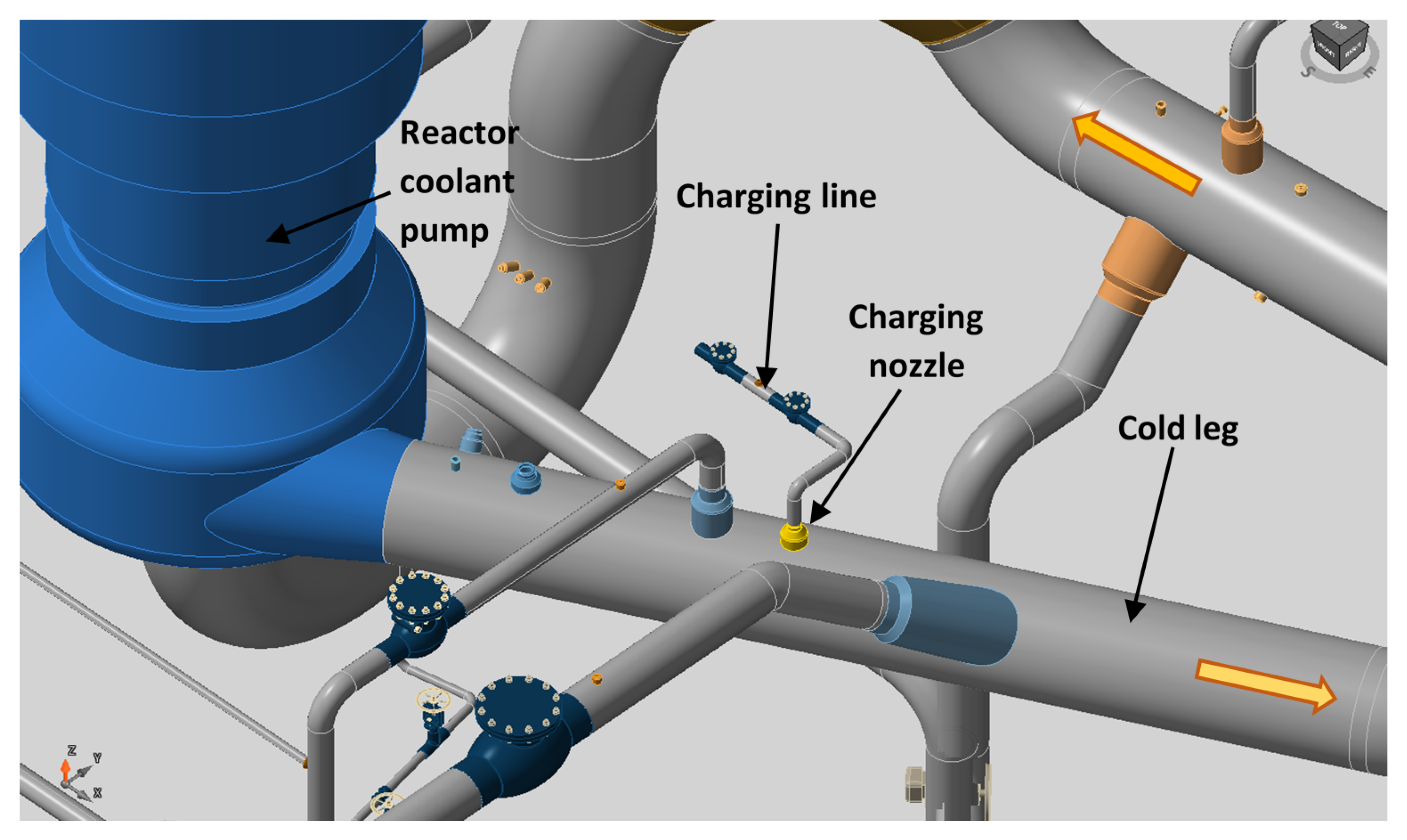
This section describes the environmental fatigue assessment (EFA) in a real nuclear structural component. More precisely, the analysis was performed in the inner radius of the charging nozzle of a PWR NPP. Figure 3 presents a scheme of the system, with the charging line, the charging nozzle, and the cold leg of the reactor coolant system (RCS), which are some of the components involved. 
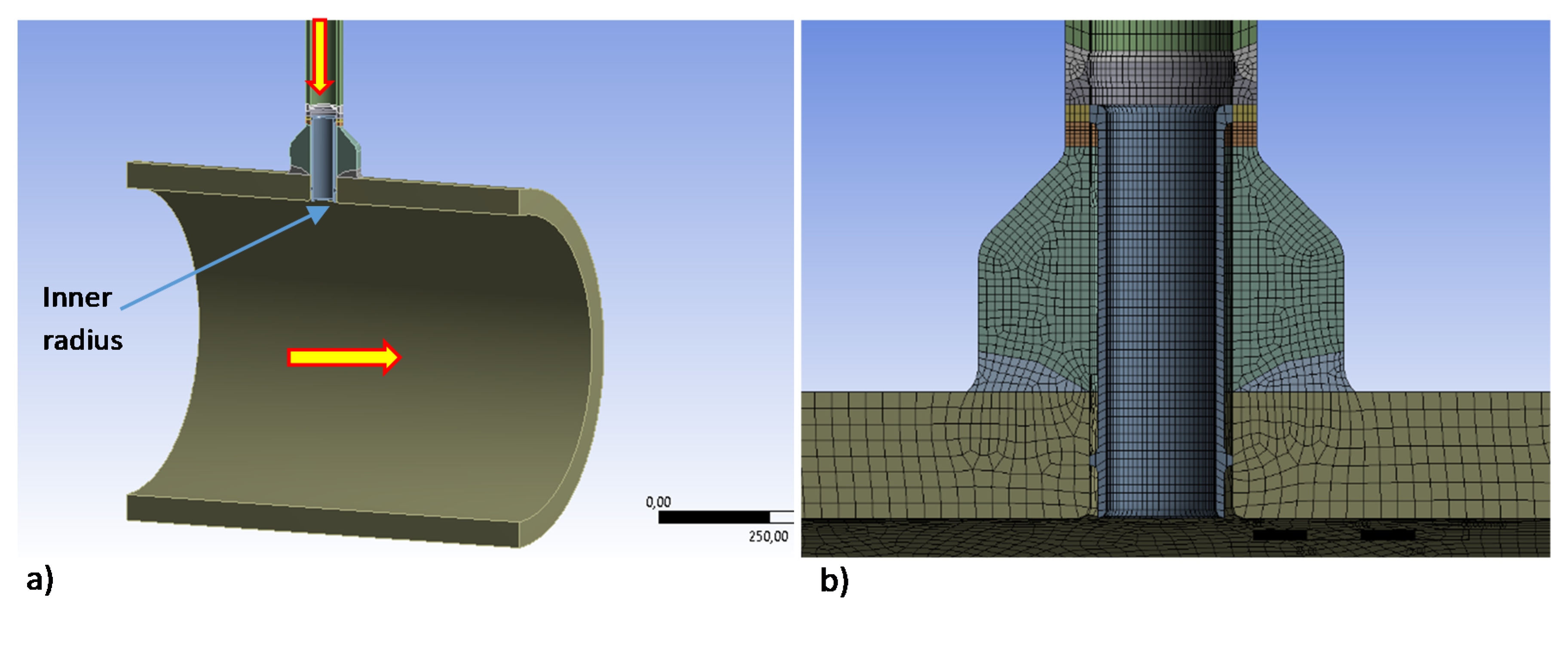
Figure 4 shows a scheme of the charging nozzle and the inner radius location at which the EFA was performed, together with the FEA model used in the stress calculation. The nozzle connects the charging line of the chemical and volume control system (CVCS) with the cold leg of the reactor coolant system (RCS) of the PWR plant. The cold leg had an inner diameter of 698.5 mm (27.5 inch) and an outer diameter of 816.34 mm (22.86 inch), whereas the inner and outer diameters of the nozzle were 66.65 mm (2.624 inch) and 88.9 mm (3.5 inch), respectively. The cold leg was made of stainless steel SA-351 Gr. CF8A and the charging nozzle was made of stainless steel SA-376 TP316, following ASME specifications.
The inner radius is typically the critical location of the charging nozzle when performing EFA. This statement has been widely validated worldwide through numerous assessments in the nuclear fleet, and has been confirmed by the stress analysis performed in this particular case, where higher stress variations appeared in such a location.
The stress report of the corresponding NPP indicates a design CUF in this inner radius location of 0.9 in 40 years.
The resulting T-joint was symmetrical in the longitudinal direction, so the FE analysis was completed by modeling one-half of the geometry. The same mesh was used to solve both thermal and mechanical problems.
Fatigue damage was analysed by using fatONE (Fatigue Management System) [38], which allows the stresses caused by design transients and real transients at critical locations to be evaluated.
Each component analysed requires the corresponding boundary conditions to be determined at every moment. These conditions are derived from the measurements provided by the instrumentation that has previously been installed in the NPP.
Temperature, pressure, and flow data defined at the design stage of the NPP are used to derive the design stresses at each particular location, whereas real-time stresses are derived from the data provided by the plant instrumentation. In both cases, FEA and the use of transference constants and Green functions are required. Finally, once the stresses are known (design stresses or real stresses), it is possible to complete the fatigue assessment.
When dealing with EFA, fatONE is able to implement different expressions of Fen. In this case, the NUREG/CR-6909 Rev.0 [14] formulation provided for stainless steels was used, together with the NUREG/CR-6909 new design fatigue curve for stainless steels in air (Table 9 in [14]):
Fen = exp(0.734-TO*·(/dt)*),
with
T* = 0, (T < 150 °C)
T* = (T−150)/175, (150 ≤ T < 325 °C)
T* = 1, (T ≥ 325 °C)
(/dt)* = 0, (/dt > 0.4%/s)
(/dt)* = ln((/dt)/0.4), (0.0004 > /dt < 0.4%/s)
(/dt)* = ln(0.0004/0.4), (/dt < 0.0004%/s)
O* = 0.281, (all dissolved oxygen levels).
T is the working temperature, /dt is the strain rate, and O is the dissolved oxygen (DO) (0.04 ppm in the cases analysed). Quantification of the differences obtained when using other Fen expressions provided by alternative procedures may be consulted in [39]. Such differences are generally very moderate, although significant variations (up to 80%) have been detected for some particular cases. In the case of austenitic stainless steel 304L, a difference of 30% was observed in the worst case [39].
This case study evaluates two sequences of transients and, additionally, these transients were analysed as design transients and real transients. Therefore, four EFAs have been completed.
The first sequence, which is more simple, consists of a cool-down, followed by a heat-up, process. The second sequence corresponds to a whole cycle of the plant for two refueling operations (18 months). Table 1 presents the list of transients and the number of design occurrences for this particular NPP.
Table 2 shows the transients of the second sequence (the first sequence is straightforward, with transients A and B).
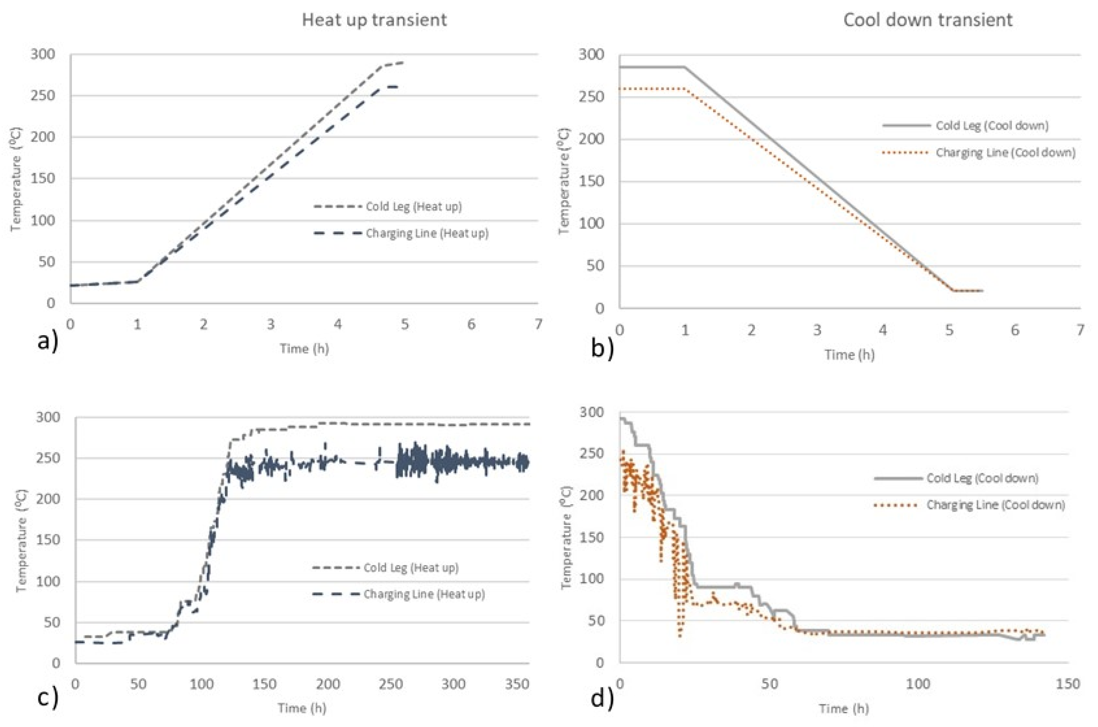
Figure 5 shows a comparison of the design and real (in-plant) transients (heat-up and cool-down). It can be observed that real transients have a longer duration than design transients: design transients usually take 5 h, while real heat-ups may take up to 3 days and cool-downs may take up to 2 days for the NPP concerned here. 
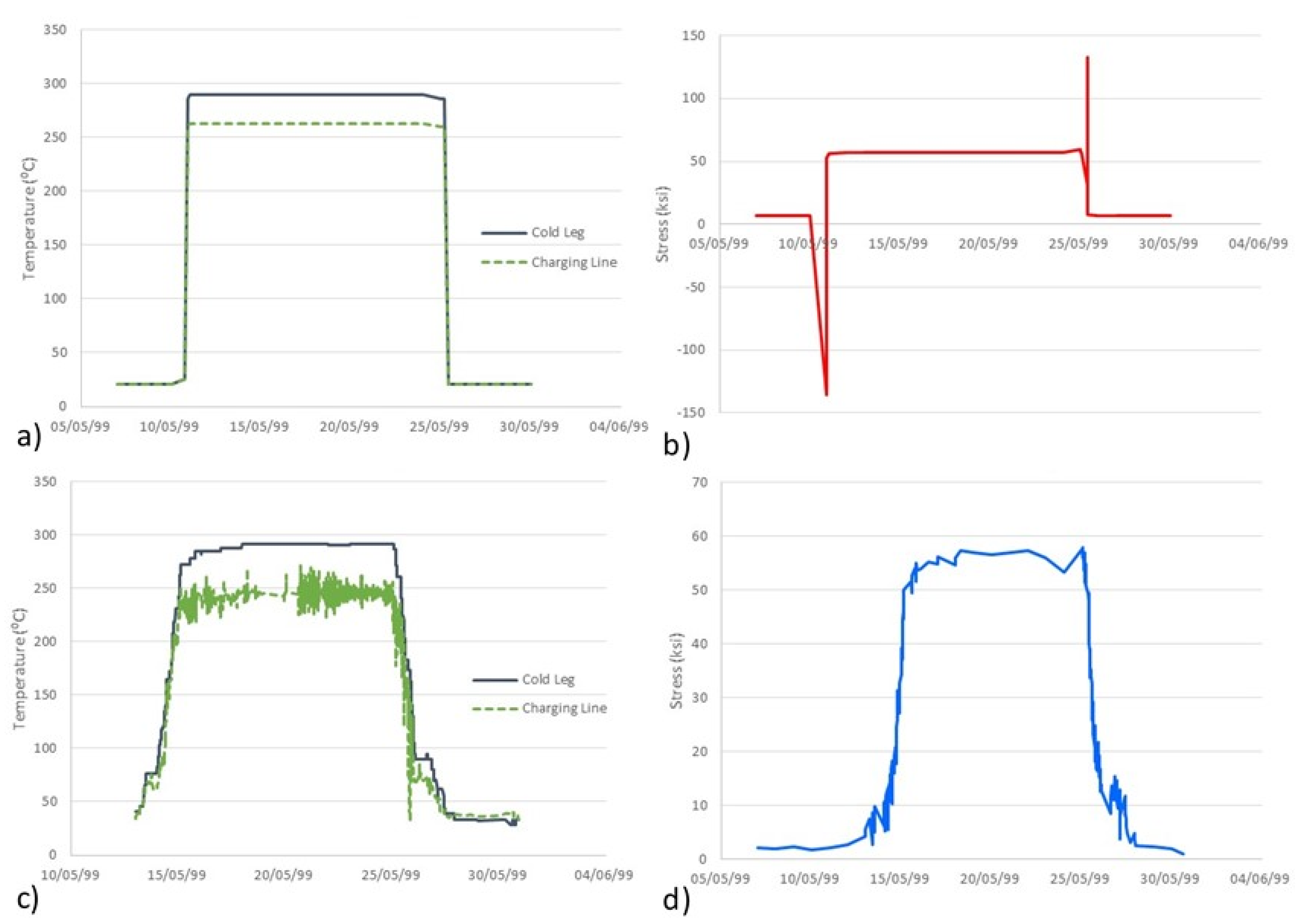
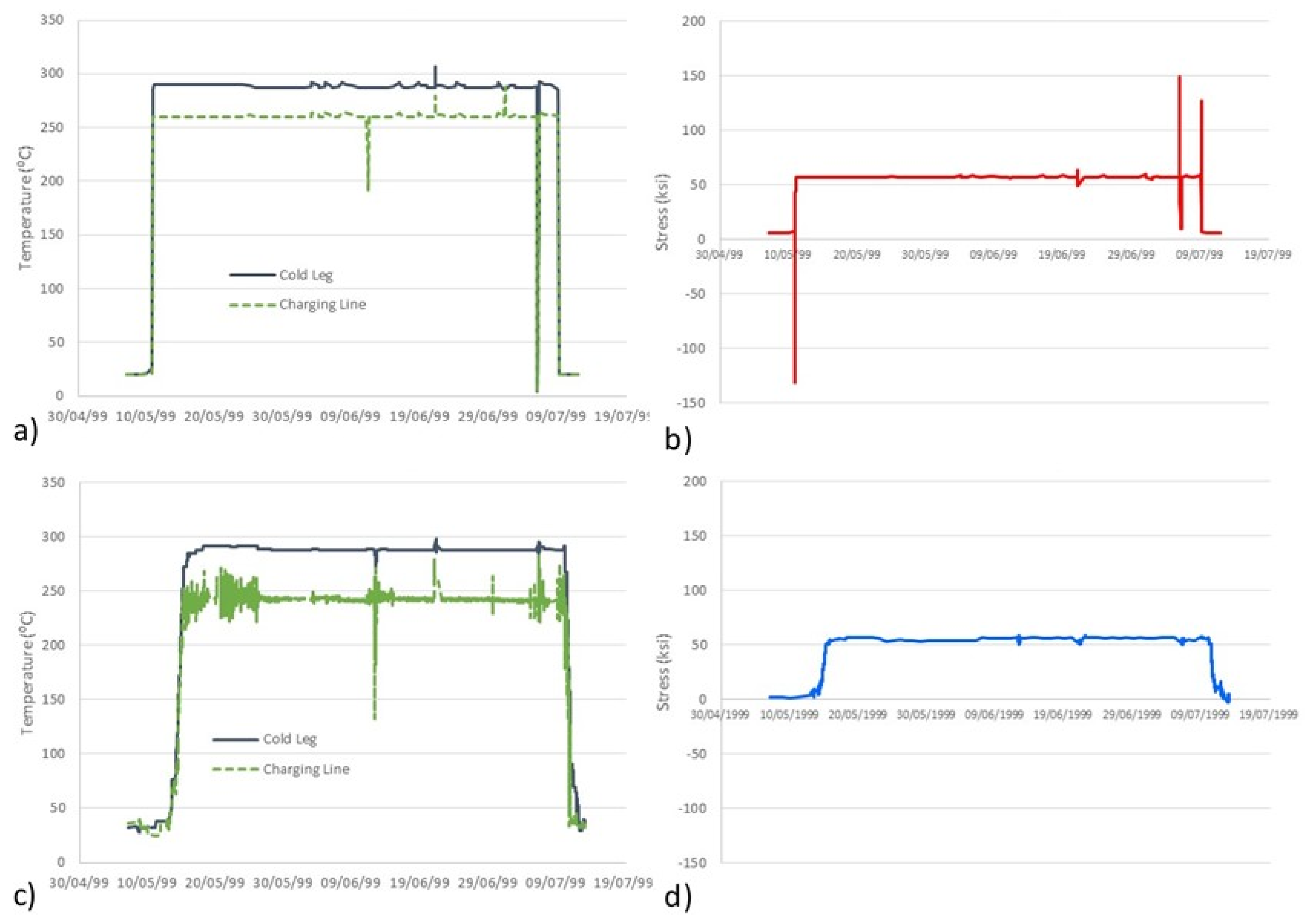
Figure 6 shows the corresponding evolution of the temperature and one of the stress components in the component being analysed during the heat-up cool-down sequence. It is important to notice how the use of Green functions in combination with abrupt transients (e.g., design transients) leads to significant stress peaks that do not appear when the transients take longer times (e.g., actual transients). Likewise, Figure 7 shows the evolution of temperature and one stress component during the second sequence of transients. Beyond the different durations of the transients (which directly affect the strain rate and, thus, the Fen factor), the stress values derived in the analyses exhibit peak values (then, stress ranges) which are significantly different when considering design and real (in-plant) transients.
Considering this, the EFA could be completed. As mentioned above, the assessment followed NUREG/CR-6909 [14]. Table 3 shows the resulting CUFs, with the different intermediate results gathered in Appendix B. The term CUF refers to the cumulative usage factor without any consideration of environmental effects, and CUFen refers to the cumulative usage factor considering the environmental effects (CUFen = CUF·Fen). Cycle counting was performed by employing the Rainflow approach, following the guidelines presented in [40].
A sharp reduction can be observed in the CUF obtained when using real data from monitoring systems. When the environmental effect is not measured, the consideration of real stresses reduces the CUF by a factor of 620 (first sequence) or 271 (second sequence); when the environmental effect is considered through the Fen factor, the CUFen factor is reduced by a factor of 1785 (first sequence) or 816 (second sequence). Therefore, for the cases analysed here, the consideration of real data (vs. design data) not only reduces the loads (and stress ranges) used in fatigue analysis, but also reduces the environmental effects through a lower Fen factor. All this has evident consequences for the structural integrity assessment of the components and demonstrates the overconservatism associated with the use of design transients.

5. Conclusions

When performing environmental fatigue assessments (EFAs) of nuclear components, it is (technically) possible to use a wide range of technical documents or standards. Moreover, load inputs may be derived from design transients or from real data captured by monitoring systems. This paper has provided an overview of the different EFA procedures, providing a comprehensive scheme on their different hypotheses, assumptions, and ways of dealing with environmental effects. The paper has also provided an explanation of the benefits of considering real data derived from real transients instead of design data derived from design transients.
It finally includes a case study in which an environmental fatigue assessment is performed for two sequences of transients in a particular location (inner radius) of a nuclear structural component (charging nozzle). The assessments follow NUREG/CR-6909, and were completed by using both real and design data. It has been demonstrated how the cumulative usage factor (CUF and CUFen) is drastically reduced when using real loads provided by monitoring systems. In this case, when no environmental effects are considered, the CUF obtained using real data is approximately two orders of magnitude times lower than that obtained from design transients, for the two sequences of transients considered here. When environmental effects are considered through the Fen factor methodology, the CUFen obtained using real transients is around three orders of magnitude lower that that derived from design transients.

Author Contributions

Conceptualization, S.C. (Sergio Cicero); methodology, S.C. (Sergio Cicero), S.C. (Sam Cuvillez), T.M., S.A., Y.V., and R.C.; software, Y.V. and R.C.; validation, S.C. (Sergio Cicero) Y.V., and R.C.; formal analysis, S.C. (Sergio Cicero), S.C. (Sam Cuvillez), T.M., S.A., Y.V., and R.C.; investigation, S.C. (Sergio Cicero), S.C. (Sam Cuvillez), T.M., S.A., Y.V., and R.C.; writing—original draft preparation, S.C. (Sergio Cicero) and T.M.; writing—review and editing, S.C. (Sergio Cicero), S.C. (Sam Cuvillez), T.M., S.A., Y.V., and R.C. All authors have read and agreed to the published version of the manuscript.

Funding

This research was funded by EURATOM, grant number 662320.

Conflicts of Interest

The authors declare no conflict of interest.

Appendix A

Table A1. Overview of the different EFA approaches.
Approach Former Fatigue CurvesNUREG/CR-6909CC
N-761
EN-13445 (Non- Weld.)EN-13445 (Weld)RCC-M DCFS KTA
Cases used or future useOver past 50 years to design PWR NPPFor license extension in USAN/ANon-nuclear industries & some conventional island componentsFor EDF NPP life extensionN/AFatigue monitoring in Germany
Data fitting equationLanger equationSpecific fitting eq. including UTSBasquin eq.Langer equation
Fatigue curveMean air curve with total least squares fitMean air curve with total least square fit and endurance determined separatelyMean air curve with total least squares fitMean air curve with total least squares fit and endurance determined separatelyMean air curve with total least squares fit
Gap between laboratory and componentLifeTranslation coefficients with multiplicationAggravating effects ranges with statistical combination Factor on life and cycles (safety factor or 3 standard deviation of data scatter) + explicit factor for aggravating parametersAggravating effects ranges with statistical combinationFactor for data scatter (β on cycles) + factor surface roughnessAggravating effects ranges with statistical combination
Strain amplitudeHighest coefficient identified through literature reviewHighest coefficient identified as being data scatter – Evaluation of its value through statistical approachesFactor for data scatter (α on stress) + factor surface roughnessMultiplication of factors taken from EN-13445 and coefficient on data scatter
Mean stressGoodman correctionFactor fm to account for mean stressN/AGoodman correctionSmith-Watson-Topper correctionsFactor from EN-13445
Environmental effectsN/AFen factor determined through study of data trendsIntegrated as part of the fatigue curve through a factor on lifeN/AFen NUREG/CR-6909 + Fen-integrated criteria determined through French testing campaignsFen factor determined through study of data trends (JNES)EAF thresholds on the usage factor + use of Fen factor with a transferability factor to include realistic conditions

Appendix B

Table A2. Calculations performed to derive the cumulative usage factor (CUF) and the cumulative usage factor considering the environmental effects (CUFen) in the first sequence of design transients. ΔSp: total stress range in the pair; ΔSn: primary + secondary stress range in the pair; Ke: elastic-plastic penalty factor; Salt: alternative stress; N: number of cycles; Na: maximum number of allowable cycles.
Cycle StartCycle EndΔSpΔSnKeSaltNNaCUFFenCUFen
07/05/1999 00:00:0010/05/1999 21:56:59146.254.30176.870.528771.737·10−411.737·10−4
10/05/1999 21:56:5925/05/1999 09:41:54275.894.752.54368.60.5598.465·10−39.207.792·10−2
25/05/1999 00:00:0025/05/1999 09:06:0929.7925.65116.4811,933,8755.170·10−715.170·10−7
25/05/1999 09:41:5426/05/1999 00:00:00129.541.42164.990.550829.838·10−519.838·10−5
-------Total8.74·10−3-7.82·10−2
Table A3. Calculations performed to derive CUF and CUFen in the first sequence of real transients. ΔSp: total stress range in the pair; ΔSn: primary + secondary stress range in the pair; Ke: elastic-plastic penalty factor; Salt: alternative stress; N: number of cycles; Na: maximum number of allowable cycles.
Cycle StartCycle EndΔSpΔSnKeSaltNNaCUFFenCUFen
07/05/1999 00:00:0025/05/1999 01:36:0058.5452.34130.780.573,6336.790·10−65.373.646·10−5
25/05/1999 01:36:0030/05/1999 15:24:0959.6452.77131.370.568,5727.291·10−617.291·10−6
-------Total1.41·10−5-4.38·10−5
Table A4. Calculations performed to derive CUF and CUFen in the second sequence of design transients. ΔSp: total stress range in the pair; ΔSn: primary + secondary stress range in the pair; Ke: elastic-plastic penalty factor; Salt: alternative stress; N: number of cycles; Na: maximum number of allowable cycles.
Cycle StartCycle EndΔSpΔSnKeSaltNNaCUFFenCUFen
07/05/1999 00:00:0010/05/1999 21:56:59141.379.821.77131.70.55968.389·10−418.389·10−4
10/05/1999 21:56:5906/07/1999 00:05:10288.9151.73.33506.20.5311.628·10−28.461.378·10−1
21/06/1999 03:35:3921/06/1999 03:35:5615.3318.1918.4991-010
06/07/1999 00:05:1006/07/1999 07:17:00142.397.462.69202.20,52162.315·10−312.315·10−3
06/07/1999 03:05:0006/07/1999 03:55:0015.928.19918.0691-010
06/07/1999 04:05:0006/07/1999 04:55:0032.6319.66116.8711,669,7195.989·10−715.989·10−7
06/07/1999 05:05:0006/07/1999 05:55:0034.8223.25118.381972,8741.027·10−611.027·10−6
06/07/1999 06:05:0006/07/1999 06:55:0036.7526.49119.831624,5021.601·10−611.601·10−6
06/07/1999 07:17:0009/07/1999 05:01:54121.089.772.30146.60.54561.095·10−39,099.963·10−3
09/07/1999 00:07:3809/07/1999 04:40:1935.1339.80119.381714,8161.398·10−611.398·10−6
09/07/1999 05:01:5410/07/1999 00:00:00124.457.14162.390.558508.547·10−518.547·10−5
-------Total2.06·10−2-1.51·10−1
Table A5. Calculations performed to derive CUF and CUFen in the second sequence of real transients. ΔSp: total stress range in the pair; ΔSn: primary + secondary stress range in the pair; Ke: elastic-plastic penalty factor; Salt: alternative stress; N: number of cycles; Na: maximum number of allowable cycles.
Cycle StartCycle EndΔSpΔSnKeSaltNNaCUFFenCUFen
07/05/1999 00:00:0012/06/1999 06:59:0059.8673.221.4244.340.518,7372.668·10−55.121.366·10−4
12/06/1999 06:59:0012/07/1999 22:20:0064.4876.221.5653.020.510,2444.880·10−514.880·10−5
-------Total7.55·10−5-1.85·10−4

References

  1. Rothenhöfer, H.; König, G. Managing Environmental Fatigue of the Real Components in a PWR. In Proceedings of the ASME 2010 Pressure Vessels and Pipping Conference, Bellevue, WA, USA, 18–22 July 2010; PVP2010-25979; American Society of Mechanical Engineers: New York, NY, USA, 2010; pp. 247–254. [Google Scholar]
  2. Nakamura, T.; Miyama, S. Environmental Fatigue Evaluation in PLM Activities of PWR plant. E-J. Adv. Maint. 2010, 2, 82–100. [Google Scholar]
  3. Chopra, O.K.; Stevens, G.L. Effect of LWR Coolant Environments on the Fatigue Life of Reactor Materials; NUREG/CR-6909 Rev.1, Final Report; U.S. Nuclear Regulatory Commission: Rockville, MD, USA, 2018.
  4. Mottershead, K.; Bruchhausen, M.; Cuvilliez, S.; Cicero, S. INCEFA-PLUS Increasing Safety in Nuclear Power Plants by Covering Gaps in Environmental Fatigue Assessment. In Proceedings of the ASME 2019 Pressure Vessels and Piping Conference, San Antonio, TX, USA, 14–19 July 2019; Volume 1A: Codes and Standards, PVP2019-93276; American Society of Mechanical Engineers: New York, NY, USA, 2019. [Google Scholar]
  5. Office of Nuclear Reactor Regulation. Standard Review Plan for Review of License Renewal Applications for Nuclear Power Plants; Final Report (NUREG-1800, Revision 2); U.S. Nuclear Regulatory Commission: Rockville, MD, USA, 2010.
  6. Office of Nuclear Reactor Regulation. Regulatory Guide 1.207: Guidelines for Evaluating Fatigue Analyses Incorporating the Life Reduction of Metal Components Due to the Effects of the Light-Water Reactor Environment for New Reactors; U.S. Nuclear Regulatory Commission: Rockville, MD, USA, 2007.
  7. Solin, J.; Reese, S.; Karabaki, H.E.; Mayinger, W. Fatigue of stainless steel in simulated operational conditions: Effects of PWR water, temperature and holds. In Proceedings of the ASME 2014 Pressure Vessels and Pipping Conference, Anaheim, CA, USA, 20–24 July 2014; Volume 1: Codes and Standards, PVP2014-28465; American Society of Mechanical Engineers: New York, NY, USA, 2014. [Google Scholar]
  8. Solin, J.; Reese, S.H.; Karabaki, H.E.; Mayinger, W. Research on hold time effects in fatigue of stainless steel: Simulation of normal operation between fatigue transients. In Proceedings of the ASME 2015 Pressure Vessels and Piping Conference, Boston, MA, USA, 19–23 July 2015; Volume 1A: Codes and Standards, PVP2015-45098; American Society of Mechanical Engineers: New York, NY, USA, 2015. [Google Scholar]
  9. Mehta, H.S.; Gosselin, S.R. Environmental Factor Approach to Account for Water Effects in Pressure Vessel and Piping Fatigue Evaluations. Nucl. Eng. Des. 1998, 181, 175–197. [Google Scholar] [CrossRef]
  10. Nuclear Boiler and Pressure Vessel Code—Section III, 2007 ed.; American Society of Mechanical Engineers: New York, NY, USA, 2007.
  11. RCC-M, Règles de Construction et de Conception des Matériel Mécaniques de l´îlot Nucléaires REP, 2007 ed.; AFCEN: Courbevoie, France, 2007.
  12. Langer, B. Design of Pressure Vessels for Low-Cycle Fatigue. J. Basic Eng. 1962, 84, 389–399. [Google Scholar] [CrossRef]
  13. Chopra, O.K.; Shack, W.J. Effect of LWR Coolant Environments on the Fatigue Life of Reactor Materials; NUREG/CR-6909 Rev.0, ANL-06/08; U.S. Nuclear Regulatory Commission: Rockville, MD, USA, 2007.
  14. Chopra, O.K.; Stevens, G.L. Effect of LWR Coolant Environments on the Fatigue Life of Reactor Materials; NUREG/CR-6909 Rev.1 DRAFT ANL-12/60; U.S. Nuclear Regulatory Commission: Rockville, MD, USA, 2014.
  15. Hald, A. Statistical Theory with Engineering Applications; John Wiley and Sons: Hoboken, NJ, USA, 1967. [Google Scholar]
  16. ASME Code Case N-761, Fatigue Design Curves for Light Water Reactor (LWR) Environments, Section III, Division 1; American Society of Mechanical Engineers: New York, NY, USA, 2010.
  17. ASME Code Case N-792-1, Fatigue Evaluation Including Environmental Effects, Section III, Division 1; American Society of Mechanical Engineers: New York, NY, USA, 2010.
  18. O’Donnell, W.J.; O’Donnell, W.J.; O’Donnell, T.P. Proposed New Fatigue Design Curves for Austenitic Stainless Steels, Alloy 600 and Alloy 800. In Proceedings of the ASME 2005 Pressure Vessels and Piping Conference, Denver, CO, USA, 17–21 July 2005; PVP2005-71409; American Society of Mechanical Engineers: New York, NY, USA, 2005; pp. 109–132. [Google Scholar]
  19. EN 13445-3 version V1, Unfired Pressure Vessels—Part 3: Design; European Committee for Standardization: Brussels, EU, USA, 2014.
  20. Wilhelm, P.; Steinmann, P.; Rudolph, J. Fatigue strain-life behavior of austenitic stainless steels in pressurized water reactor environments. In Proceedings of the ASME 2015 Pressure Vessels and Piping Conference, Boston, MA, USA, 19–23 July 2015; Volume 1A: Codes and Standards, PVP2015-45011; American Society of Mechanical Engineers: New York, NY, USA, 2015. [Google Scholar]
  21. AD 2000 Merkblatt S2: 2012, Analysis for Cyclic Loading; German Institute for Standardisation: Berlin, Germany, 2012.
  22. Haibach, E. Betriebsfestigkeit: Verfahren und Daten zur Bauteilberechnung, 3rd ed.; Springer: Berlin/Heidelberg, Germany, 2006. [Google Scholar]
  23. Métais, T.; Courtin, S.; Genette, P.; De Baglion, L.; Gourdin, C.; Le Roux, J.C. Overview of French Proposal of Updated Austenitic SS Fatigue Curves and of a Methodology to Account for EAF. In Proceedings of the ASME 2015 Pressure Vessels and Piping Conference, Boston, MA, USA, 19–23 July 2015; Volume 1A: Codes and Standards, PVP2015-45158; American Society of Mechanical Engineers: New York, NY, USA, 2015. [Google Scholar]
  24. Le Duff, J.A.; Lefrançois, A.; Vernot, J.P.; Bossu, D. Effect of loading signal shape and of surface finish on the low cycle fatigue behavior of 304L stainless steel in PWR environment. In Proceedings of the ASME 2010 Pressure Vessels and Pipping Conference, Bellevue, WA, USA, 18–22 July 2010; PVP2010-26027; American Society of Mechanical Engineers: New York, NY, USA, 2010; pp. 233–241. [Google Scholar]
  25. Blatman, G.; Métais, T.; Le Roux, J.C.; Cambier, S. Statistical analyses of high cycle fatigue French data for austenitic SS. In Proceedings of the ASME 2014 Pressure Vessels and Pipping Conference, Anaheim, CA, USA, 20–24 July 2014; Volume 3: Design and Analysis, PVP2014-28409; American Society of Mechanical Engineers: New York, NY, USA, 2014. [Google Scholar]
  26. JSME. Codes for Nuclear Power Generation Facilities, Rules on Design and Construction for Nuclear Power Plants, the First Part: Light Water Reactor Structural Design Standard, JSME S NC1-2008 ed.; The Japan Society of Mechanical Engineers: Tokyo, Japan, 2008. [Google Scholar]
  27. Kanasaki, H.; Higuchi, M.; Asada, S.; Yasuda, M.; Sera, T. Proposal of Fatigue Life Equations for Carbon & Low-Alloy Steels and Austenitic Stainless Steels as a Function of Tensile Strength. In Proceedings of the ASME 2013 Pressure Vessels and Piping Conference, Paris, France, 14–18 July 2013; Volume 1A: Codes and Standards, PVP2013-97770; American Society of Mechanical Engineers: New York, NY, USA, 2013. [Google Scholar]
  28. Asada, S.; Hirano, T.; Sera, T. Study on a New Design Fatigue Evaluation Method. In Proceedings of the ASME 2015 Pressure Vessels and Piping Conference, Boston, MA, USA, 19–23 July 2015; Volume 1A: Codes and Standards, PVP2015-45089; American Society of Mechanical Engineers: New York, NY, USA, 2015. [Google Scholar]
  29. Asada, S.; Zhang, S.; Takanashi, M.; Nomura, Y. Study on Incorporation of a New Design Fatigue Curve into the JSME Environmental Fatigue Evaluation Method. In Proceedings of the ASME 2019 Pressure Vessels and Piping Conference, San Antonio, TX, USA, 14–19 July 2019; Volume 3: Design and Analysis, PVP2019-93273; American Society of Mechanical Engineers: New York, NY, USA, 2019. [Google Scholar]
  30. ISO 4287:1997, Geometrical Product Specifications (GPS)—Surface Texture: Profile Method—Terms, Definitions and Surface Texture Parameters; The International Organization for Standardization: Geneva, Switzerland, 1997.
  31. JNES-SS-1005, Environmental Fatigue Evaluation Method for Nuclear Power Plants; Japan Nuclear Energy Safety Organization: Tokyo, Japan, 2011.
  32. KTA 3201.2 (2017-11) Components of the Reactor Coolant Pressure Boundary of Light Water Reactors Part 2: Design and Analysis; KTA-Geschaeftsstelle: Salzgitter, Germany, 2017.
  33. Schuler, X.; Herter, K.H.; Rudolph, J. Derivation of Design Fatigue Curves for Austenitic Stainless Steel Grades 1.4541 and 1.4550 within the German Nuclear Safety Standard KTA 3201.2. In Proceedings of the ASME 2013 Pressure Vessels and Piping Conference, Paris, France, 14–18 July 2013; Volume 1B: Codes and Standards, PVP2013-97138; American Society of Mechanical Engineers: New York, NY, USA, 2013. [Google Scholar]
  34. Reese, S.H.; Rudolph, J. Environmentally Assisted Fatigue (EAF) Rules and Screening Options in the Context of Fatigue Design Rules within German Nuclear Safety Standards. In Proceedings of the ASME 2015 Pressure Vessels and Piping Conference, Boston, MA, USA, 19–23 July 2015; Volume 6A: Materials and Fabrication, PVP2015-45022; American Society of Mechanical Engineers: New York, NY, USA, 2015. [Google Scholar]
  35. Ware, A.G.; Morton, D.K.; Nitzel, M.E. Application of NUREG/CR-5999 Interim Fatigue Curves to Selected Nuclear Power Plant Components; NUREG/CR-6260 INEL-95/0045; Idaho National Engineering Laboratory: Idaho Falls, ID, USA, 1995.
  36. Cicero, R. Evaluación del Gasto en Fatiga de Vasijas a Presión de Reactors Nucleares Considerando el Efecto Ambiental Mediante el Empleo de Datos Reales. Ph.D. Thesis, Universidad de Cantabria, Santander, Spain, 2013. [Google Scholar]
  37. Software Specifications for FatiguePro, 3rd ed.; Structural Integrity Associates Report Nº SIR-99-051, Revision 1, SI File n EPRI.136Q-401; Structural Integrity Associates: San Jose, CA, USA, 2001.
  38. Software fatONE, Fatigue Management System, version 3.1.9577; Innomerics, S.L.: Madrid, Spain, 2020.
  39. Hannink, M.H.C.; Blom, F.J.; Quist, P.W.B.; de Jong, A.E.; Besuijen, W. Demonstration of Fatigue for LTO License of NPP Borssele. In Proceedings of the ASME 2015 Pressure Vessels and Piping Conference, Boston, MA, USA, 19–23 July 2015; Volume 3: Design and Analysis, PVP2015-45791; American Society of Mechanical Engineers: New York, NY, USA, 2015. [Google Scholar]
  40. Gray, M.A.; Verlinich, M.M. Guidelines for Addressing Environmental Effects in Fatigue Usage Calculations; Electric Power Research Institute (EPRI): Palo Alto, CA, USA, 2012. [Google Scholar]
Figure 1. Fatigue curves for non-welded components in EN-13445 (reproduced from [19], European Committee for Standardization, 2014). The different fatigue curves each correspond to a different ultimate tensile strength (UTS) level. The dashed lines correspond to fatigue endurance limits in the case of variable amplitude loads [19]. ΔσR represents the stress range.
Metals 10 00609 g001
Figure 2. (a) Evolution of a particular stress component provided by a monitoring system in a Safe End; (b) evolution of the temperature at the same timing and location. The sequence includes six consecutive design transients (corresponding to the different colored lines) [36].
Metals 10 00609 g002
Figure 3. Scheme of the different components involved and location of the charging nozzle within the whole system. Yellow arrows indicate the direction of flow.
Metals 10 00609 g003
Figure 4. (a) Scheme of the charging nozzle and the cold leg, with the inner radius location. (b) FE model used in stress analysis. Yellow arrows indicate the direction of flow.
Metals 10 00609 g004
Figure 5. Temperature evolution in both the cold leg and the charging line during design and in-plant transients. (a) Design heat-up; (b) design cool-down; (c) in-plant heat-up; (d) in-plant cool-down.
Metals 10 00609 g005
Figure 6. Temperature and stress evolution in both the cold leg and the charging line during the first sequence of transients. (a) Design temperature; (b) design stresses; (c) in-plant temperature; (d) in-plant stresses. Dates on the horizontal axes do not necessarily correspond to actual dates.
Metals 10 00609 g006
Figure 7. Temperature and stress evolution in both the cold leg and the charging line during the second sequence of transients. (a) Design temperature; (b) design stresses; (c) in-plant temperature; (d) in-plant stresses. Dates on the horizontal axes do not necessarily correspond to actual dates.
Metals 10 00609 g007
Table 1. Transients considered in the analysis and design occurrences.
TransientDescriptionDesign Occurrences
AHeat-up at 100 °F/h200
BCool-down at 100 °F/h200
CUnit loading at 5% of full power/min18,300
DUnit unloading at 5% of full power/min18,300
ELoss of load from full power80
FReactor trip from full power400
GCharging rate increased by 50%24,000
HLetdown rate decreased by 50%2000
ICharging rate decreased by 50%24,000
JHigh head safety injection50
Table 2. Transients of the second sequence. Dates do not necessarily correspond to actual dates, but the sequence itself, the distribution over time, and the duration of transients correspond to real data.
TransientStartEndName
A10/05/1999 17:10:0002/06/1999 02:46:00Heat-up at 100 F/h
C25/05/1999 20:18:0029/05/1999 13:12:00Unit loading at 5% of full power/min
D03/06/1999 00:57:0003/06/1999 20:11:00Unit unloading at 5% of full power/min
C04/06/1999 00:16:0004/06/1999 16:15:00Unit loading at 5% of full power/min
D05/06/1999 00:30:0005/06/1999 09:36:00Unit unloading at 5% of full power/min
C05/06/1999 19:23:0006/06/1999 05:31:00Unit loading at 5% of full power/min
D07/06/1999 08:36:0007/06/1999 10:46:00Unit unloading at 5% of full power/min
D08/06/1999 09:21:0008/06/1999 12:52:00Unit unloading at 5% of full power/min
D09/06/1999 09:09:0009/06/1999 13:36:00Unit unloading at 5% of full power/min
C09/06/1999 22:04:0010/06/1999 17:13:00Unit loading at 5% of full power/min
G11/06/1999 05:02:0011/06/1999 05:16:20Charging rate increased by 50%
H11/06/1999 05:16:2011/06/1999 05:45:20Letdown rate decreased by 50%
C11/06/1999 21:51:0014/06/1999 17:50:00Unit loading at 5% of full power/min
D15/06/1999 21:45:0016/06/1999 08:38:00Unit unloading at 5% of full power/min
C16/06/1999 11:50:0017/06/1999 02:44:00Unit loading at 5% of full power/min
D18/06/1999 14:31:0019/06/1999 01:33:00Unit unloading at 5% of full power/min
D19/06/1999 09:53:0019/06/1999 17:16:00Unit unloading at 5% of full power/min
C19/06/1999 21:39:0020/06/1999 02:31:00Unit loading at 5% of full power/min
E21/06/1999 03:34:0021/06/1999 11:16:00Loss of load from full power
C22/06/1999 21:48:0023/06/1999 16:09:00Unit loading at 5% of full power/min
D24/06/1999 04:29:0024/06/1999 22:25:00Unit unloading at 5% of full power/min
C25/06/1999 08:58:0029/06/1999 12:09:00Unit loading at 5% of full power/min
D30/06/1999 07:30:0030/06/1999 18:34:00Unit unloading at 5% of full power/min
I01/07/1999 09:11:0001/07/1999 09:34:00Charging rate decreased by 50%
C02/07/1999 18:42:0005/07/1999 04:36:00Unit loading at 5% of full power/min
F06/07/1999 00:00:0008/07/1999 00:00:00Reactor trip from full power
J06/07/1999 00:05:0006/07/1999 12:40:00High head safety injection
B09/07/1999 00:00:0012/07/1999 08:57:00Cool-down at 100 F/h
Table 3. Environmental fatigue assessment (EFA) of the inner radius location for the two sequences of transients being considered.
SequenceDesign TransientsReal TransientsCUFdesig/CUFrealCUFen,desig/CUFen,real
1CUF8.74·10−31.41·10−56201785
CUFen7.82·10−24.38·10−5
Fen8.953.11
2CUF2.06·10−27.55·10−5272816
CUFen1.51·10−11.85·10−4
Fen7.332.45

