Article

Diagnosis Method for the Heat Balance State of an Aluminum Reduction Cell Based on Bayesian Network

School of Metallurgy and Environment, Central South University, Changsha 410012, China
*
Author to whom correspondence should be addressed.
Metals 2020, 10(5), 604; https://doi.org/10.3390/met10050604
Submission received: 29 March 2020 / Revised: 25 April 2020 / Accepted: 5 May 2020 / Published: 7 May 2020

Abstract

:
The superheat of an electrolyte is an important indicator of the heat balance state of aluminum reduction cells. In industrial practice, it costs too much to accurately measure the superheat in every cell every day. A common alternative is to calculate the superheat based on additive concentrations in the electrolyte, which has problems of high error and long delay. In this paper, a method to diagnose the heat balance state of an aluminum reduction cell based on Bayesian network is presented, a Bayesian network structure and CPT (conditional probability distribution) were built, and the continuous diagnosis process is presented. This diagnosis method takes important symptoms and factors into account, taking advantage of more useful information instead of only calculated superheat. The application examples show that this method is effective in diagnosing the heat balance state for uncertain and incomplete superheat information.

1. Introduction

Maintaining a proper heat balance state is of great importance for the highly efficient and stable operation of aluminum reduction cells. Technically, it is necessary to evaluate the heat balance state through a comprehensive index of electrolyte superheat and ledge thickness. Literature studies [1,2,3,4,5] show that the superheat and ledge thickness are mutually coupled, which can achieve automatic balance to some extent. When the superheat is too low, the thickness of the ledge thickness increases, which causes the superheat to rise again. When the superheat is too high, the thickness of the ledge decreases, which causes the superheat to decrease again. When the heat balance changes, superheat responds very fast, while the ledge thickness responds much slower. In most cases, representing heat balance state only through the superheat does not cause big errors.
Although many researchers and companies have developed instruments to measure superheat, they are not yet widely used in practical production due to the high price and complex operation requirements. Technicians in most aluminum smelters make indirect estimates of superheat by applying the following methods: sampling electrolyte and making the electrolyte composition analysis in the laboratory, then calculating the liquidus temperature according to the empirical formula, and then subtracting the liquidus temperature from the electrolyte temperature to obtain the superheat. This method is not good in time-effectiveness, and has large errors in analyzing electrolyte composition. In order to compensate, the technician also judges the heat balance state with the aid of some signs. There are several heat balance states, including low superheat cell, normal cell, and high superheat cell. When the superheat is too low, the cell is regarded as a low superheat cell, presenting decreasing cell temperature, poor alumina dissolution, more precipitation and anode effects, amongst others. When the superheat is too high, the cell is regarded as a high superheat cell, presenting increasing temperature, sidewall redness, decreasing current efficiency, among other effects.
The development of the machine learning model in recent years has led many scholars to apply it to the prediction of the superheat, electrolyte temperature, and control system in aluminum reduction cells. Guo [6] proposed a time granularity-based superheat prediction model, with feature sets and training sets built on different time series. Based on the Restreken formula, Cao [7] proposed making corrections to the composition by using recent historical measurements in compliance with the relevant law of volatile composition consumption, and improved the empirical prediction formula of the liquidus temperature, which can be used to estimate the superheat in the non-sampling period. Long [8], Ding [9], Li [10], and Boadu [11], amongst others, improved the alumina feeding control system by using the BP neural network or fuzzy neural network. Frost and Karri [12,13] studied the method to predict and control the electrolyte temperature through BP neural network. In Zheng’s research [14,15], neural network was applied in aluminum fluoride addition and cell status diagnosis. Li [16,17], and Li [18], amongst others, combined wavelet theory with neural network to establish a reduction cell state prediction model.
Although artificial neural network has received much attention from many researchers, there are many limits of application in predicting heat balance state due to the high technicality and complexity of artificial neural network. Compared with artificial neural network, another machine learning model, the Bayesian network, has been used very successfully in many industries and fields, particularly in the medical industry. Bayesian network is a probability network model based on the causality among variables, which has unique advantages in describing the complex causality between cause and signs. The technique mentioned above uses the various signs to judge low or high superheat cells by experience, whose basic idea is consistent with the principle of the Bayesian network. This paper analyzes the causality between the related variables of the heat balance state, on the basis of which the Bayesian network is established, calculating the conditional probability distribution from the manual measurement and online measurement data, thus proposing the specific continuous diagnosis procedures.

2. Bayesian Network

Bayesian network is a type of probabilistic graphical model based on Bayesian theorem, which is a directed acyclic graph containing nodes and directed edges. The directed edge represents the causality or association among nodes. The association strength is determined by the conditional probability table. Generally speaking, Bayesian theorem is that you can predict the probability of an event relying on the probability of other events related to the nature of the event when you can’t determine the probability of an event occurrence. As mathematicians say, the more events supporting an attribute occur, the greater the likelihood that it will occur [19].

2.1. Selection of Network Node

There are many variables during aluminum reduction. It is necessary to select variables with obvious causality with heat balance state as nodes of Bayesian network. Through state discretization of 500 kA cell production data in a Chinese smelter according to the actual situation and variable characteristics, the specific nodes and state discretization are listed in Table 1.
(1) “Heat_state”
This node indicates the heat balance state of the cell based on its superheat value.
(2) “Often_AE”
When the superheat decreases, alumina is not easily dissolved and more anode effects will occur, which can be acquired in the cell control system in real time.
(3) “Block”
When superheat decreases, undissolved alumina will accumulate near the feeding hole and cause blockage. If the blocked hole is not cleaned, the block is only counted once. After cleanup, if the block occurs on this hole again, another block event can be counted. An intelligent breaking and feeding system was applied to monitor the block state of each feeding hole, the method of which is in [20].
(4) “Bath_level”
This node represents the height of the bath level.
(5) “Metal_level”
This node represents the height of the metal level.
(6) “Superheat”
“Superheat” is calculated based on electrolyte temperature and liquidus temperature. The empirical formula for liquidus temperature calculation is given in the literature [21].
(7) “Heat_long”
Firstly, the current efficiency for a longer period of time (the latest week in general) is approximately current efficiency η according to tapping amount, so electrochemical reaction consumption and energy for heating materials [22] is WR = (0.48 + 1.644 × CE/100) × I (kW).
The energy input is equal to voltage times current: Win = U × I (kW).
In the above two formulas, U refers to cell voltage and I refers to potline current, both of which can be acquired from the cell control system in real time.
In accordance with the law of energy balance, the heat loss from a cell surface equals WinWR, which is also the heat for maintaining cell temperature and electrolyte superheat. This heat value is estimated based on average current efficiency for a longer period of time, so it is called “Heat_long”. For easy understanding, voltage is used to express “Heat_long”, i.e., U − (0.48 + 1.644 × CE/100).
(8) “MHD” (Magnetohydrodynamic)
The MHD fluctuation index can be acquired from anode current monitoring system. The higher the index, the more fluctuations occur between the molten metal and electrolyte interface.
(9) “CVD”
Both cathode block quality and proper heating-up process can influence cathode voltage drop (CVD), but those influence are long and stable. The value of “CVD” must be determined based on the actual conditions of each cell. After verifying that there is no hard precipitation on the cathode and that the heat balance state remains normal, CVD (V0) is measured as baseline.
(10) “Spike”
All anode currents were measured by an online anode current measuring system [23,24]. Anode current can obviously reflect the anode spike. As for the anodes with higher current and lower noise, the anode spike can be inspected on the monitor by operators.
(11) “Temp_change”
This variable represents the variation trend of bath temperature.
The temperature measurement precision of thermocouple is 0.1 °C. The three latest values of electrolyte temperatures (in chronological order T2, T1, and T0; T0 represents the temperature measured that day) are used to conduct trend analysis.
(12) “Heat_xstate”
The variable is not an observed variable but a known variable, which is a historical value of previous “Heat_state”. It is based on the manual measurement of superheat. Its classification is consistent with “Heat_state”.
(13) “Wall_temp”
This node refers to the temperature of the side wall surface.
(14) “Sludge”
The sludge on the cathode surface can be judged by operators.
(15) “Heat_present”
“Heat_present” is jointly determined by “Spike” and “Heat_long”. “Heat_present” refers to the current heat loss considering anode spikes, which is the correction of “Heat long”, so its state classification is consistent with “Heat long”.

2.2. Analysis of Causality among Nodes

2.2.1. Variables Influencing “Heat_State”

The “Heat_state” of an aluminum reduction cell is determined by two key factors: the heat loss (i.e., “Heat_present”) and thermal insulation performance. When the thermal insulation performance remains unchanged, the higher the “Heat present” is, the hotter the cell could be. When “Heat_present” remains unchanged, the better the thermal insulation is, the hotter the cell could be.
Thermal insulation is mainly influenced by the type and thickness of insulation material in the lining of the aluminum reduction cell, the thickness of the cover material on the upper part of the cell, the ventilation conditions of the external surface of the cell, the “Metal_level”, the ledge thickness, and other factors. The type and thickness of the insulation material are usually determined during the engineering stage and cannot be changed during cell operation. It is necessary to take a very long time to effectively adjust the cover material thickness of upper part of the cell. The ventilation conditions on the external surface of the cell also change very slowly unless forced ventilation is used in the event of an emergency. “Metal_level” is an important means to influence and regulate the heat balance in the normal operation of cells. Although it is not recommended that heat balance is adjusted by “Metal_level” too often, “Metal_level” is one of the available important means for smelters when there are heat balance problems. The ledge thickness is the result of the heat balance state, which is variable along with the changing of the heat balance state.
Therefore, “Heat_present” and “Metal_level” are those variables influencing “Heat_state” of aluminum reduction cells.

2.2.2. Variables Affected by “Heat_State”

(1) “Often AE”
As mentioned above, some alumina cannot be dissolved when the superheat is low, and it can easily lead to the occurrence of anode effects.
In addition, the variable “Bath level” influences “Often_AE”. When the “Bath_level” is low, i.e., insufficient electrolyte to dissolve the amount of alumina, this results in more anode effects.
As the electrolyte ratio (concentration ratio of NaF/AlF3) decreases, the saturated solubility of alumina decreases, and the alumina dissolution rate decreases as well. The current alumina concentration can generally be controlled below 3%, and the appropriately low electrolyte ratio will not cause an anode effect [25]. In addition, many aluminum smelters target achieving a low electrolyte ratio. The anode effect will occur frequently (i.e., 1 AE/pot∙day) only when the electrolyte ratio is very low. In this paper, it is assumed that the electrolyte ratio can be controlled within a reasonable range.
(2) “Superheat”
Although “Superheat” has an error in calculation, unable to exactly substitute the actual superheat, it has a certain relation with the actual superheat.
(3) “Wall_temp”
When the cell maintains high superheat, “Wall temp” will become very high.
(4) “Block”
When the cell maintains low superheat, alumina is not easily dissolved and the feeding hole is easily blocked.
(5) “Sludge”
When the cell retains low superheat for a long time, the alumina easily precipitates on the cathode surface and hard precipitation forms and, therefore, “Sludge” becomes worse.
(6) “Temp_change”
“Heat_xstate” and “Heat state” have joint influence on “Temp_change”. If the cell changes from low to high superheat, “Temp_change” presents an upward trend (i.e., state of “increase”); if the cell changes from high to low superheat, “Temp_change” presents a downward trend (i.e., state of “decrease”).
In addition, “Heat_state” can also influence “Bath level”, but such influence is ignored since the operators often tap or add electrolyte, giving rise to great disturbance on the “Bath level”.

2.2.3. Influencing of Other Variables

(1) Influence of “Sludge” on “CVD”
As “Sludge” worsens, hard precipitation increases, and area of current passing the cathode surface decreases, so the “CVD” becomes higher.
(2) Influence of “Metal_level” and “Sludge” on “MHD”
As “Metal_level” becomes lower or there is much hard precipitation on the cathode, the horizontal current in the molten metal becomes higher, which makes “MHD” more likely to be worse.
(3) Influence of “Spike” and “Heat_long” on “Heat_present”
When “Spike” occurs, a current passes through the conducting spike under the anode, which causes molten metal short circuit and no electrochemical reaction happens, so the energy consumed decreases and the corresponding “Heat present” becomes higher.

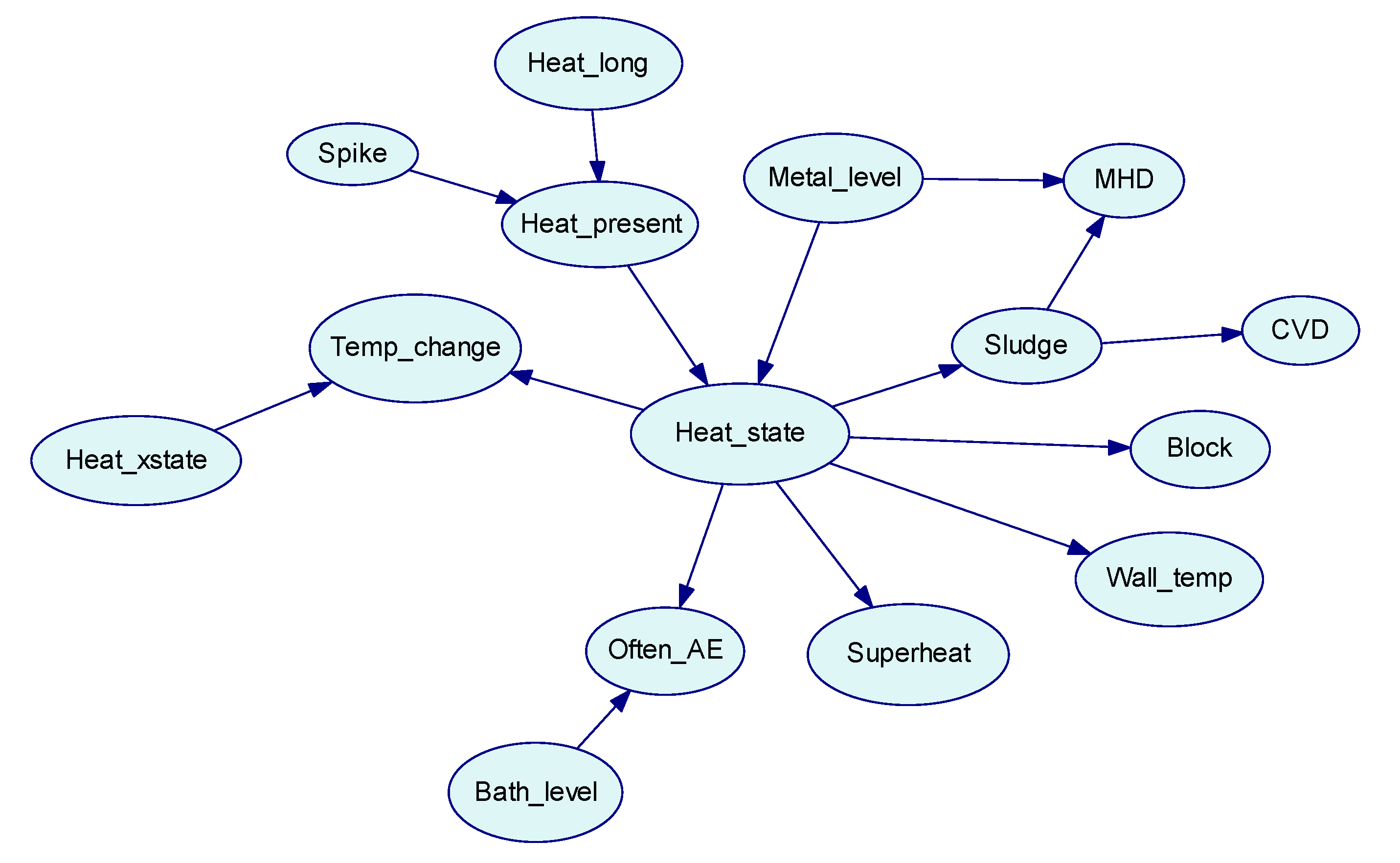
2.3. Configuration of Bayesian Network

2.3.1. Structure of Bayesian Network

Based on the above analysis of causality among different nodes, the Bayesian network can be configured as shown in Figure 1.
“Heat_present” and “Metal_level” are the parent nodes of “Heat_state”. Other factors, such as lining structure, ventilation, and anode cover thickness, are not incorporated into the Bayesian network, since these factors are more stable and are seldom used to adjust the heat balance of the cell.
The child nodes of “Heat_state” are “Temp_change”, “Often_AE”, “Superheat”, “Wall_temp”, “Block”, and “Sludge”, which give signs that are easily seen when the cell becomes low or high superheat.

2.3.2. Conditional Probability Tables

After finalizing Bayesian network structure, it is necessary to establish a conditional probability table based on known data. The data is from production reports and actual measurements (including online and manual measurements) of 500 kA cell during a three-month period in a potroom.
As mentioned above, if the equipment is used to measure the superheat of each cell on site every day, it a lot of time and costs will be spent. Setting superheat as the target variable in this model can realize timely understanding of the superheat variation at lower cost without requiring frequent daily measurement of superheat. However, if there are no measured superheat data at all, the parameter learning in the model cannot be carried out, so a small amount of superheat measurement data is required to complete the parameter learning.
By means of the automatic calculation function of GeNIe 2.3 Academic software (BayesFusion, LLC, Pittsburgh, PA, USA), the conditional probability table for each node is calculated after the original data are input. Table 2 shows a list of probability distributions of “Heat_present” and “Metal_level” to “Heat_state” conditions. The conditional probability tables of other nodes are not shown here due to space limitations.

3. Diagnosis and Analysis of Heat Balance

Bayesian network takes evidence as input variables. Evidence refers to the state value of a known variable which shall be input to the model to solve the probability distribution of other variables. It is unnecessary to treat all measurement variables as known conditions every time; instead, any part of them may be used.

3.1. Inference and Calculation Method of Bayesian Network

As for networks with n nodes such as x1, x2, …, xn, the joint probability distribution of Bayesian network is
P ( x 1 , x 2 , , x n ) = i = 1 n P ( x i | p a r e n t s ( x i ) ) .
The conditional probability of a node is related to the parent node, and ignores the nodes without a connection.
Setting A1, A2, …, An as a complete group of incompatible events for E, and P(Ai) > 0, B represents any event of E, according to the Bayesian formula:
P ( A i | B ) = P ( A ) P ( B | A i ) j = 1 n P ( A j ) P ( B | A j ) .
The probability distribution of other variables can be calculated based on the selected evidence variables as known conditions in accordance with Equations (1) and (2). Some mature commercial software or toolkits can be applied to the inference and calculation of Bayesian network. The author wrote code and conducted automatic data input and calculation based on Bayesian network Toolbox (BNT) of MATLAB 7.12.0.635 software (The MathWorks, Inc., Natick, MA, USA).

3.2. Single Diagnosis

Except for those variables not frequently measured (such as “Wall_temp” and “Sludge”), there are ten variables commonly used as evidence, which can constitute more than twenty thousand combinations, so it is impossible to list them all. Table 3 lists the diagnosis results of some typical evidence combinations.

3.3. Continuous Diagnosis

The “Superheat” is calculated based on the electrolyte composition, assuming the measurement frequency of the electrolyte composition is once every 7 days. The longer the time from the electrolyte sampling time, the greater the difference between the analytical value and the real measured value. The specific requirements of the model for the “Superheat”: If electrolyte is sampled on Day 1, the analysis results will be obtained on Day 2, which will work as evidence of the model operation on Day 2. At the same time, the probability of “Superheat” and “Heat_state” of the model are updated on Day 1, and “Superheat” is no longer used as evidence after Day 3, until the loop to the next electrolyte composition measurement date.
(1) Conditions of Continuous Diagnosis
Assuming the states of “Heat_present” and “Metal_level” are known and remain the same all the time, the continuous calculation method can be used: regarding the conditional probability of the “Heat_state” under known “Heat_present” and “Metal_level” as prior probability; regarding the probability result of “Heat_state” after calculation as posterior probability, which can be an update of the prior probability of the “Heat_state” for the next calculation.
(2) Application Cases of Continuous Diagnosis
There are three continuous calculation cases (Cases A–C) as shown in Table 3, Table 4 and Table 5. The specific calculation process is as follows: make electrolyte sample on Day 1, conduct analysis of the electrolyte composition on Day 2. On Day 2, calculate the “Heat_state” on Day 1 and Day 2 at the same time (using the same composition). From Day 3, the actual composition has a big difference with the value at the time of sampling, so the “Superheat” is not set as evidence. On Day N (N ≥ 3), the “Heat_state” result of Day N − 2 is assigned to the current “Heat_xstate” as a prior probability, and the “Heat_state” result of Day N − 1 is assigned to the current “Heat_state” as a prior probability (provided that the “Heat_state” and “Metal_level” remain unchanged; if there is a change, use the original condition probability), calculate the “Heat_state” result of Day N, and until the loop to the next composition results.
In Case A, from Day 4, evidence of “Bath_temp” presents an upward trend. On Day 4, the probability of “High” in “Heat_state” increases from 0.8% on the previous day to 11.5%, and reaches up to 68.3% and 97.2% on Day 5 and Day 6, respectively.
Case B can be obtained through modifying the evidence of “Bath_temp” in Case A from upward into downward. In Case B, the probability of “Normal” of “Heat_state” is maintained above 98% all the time, and the probability of “Low” only slightly increases. The phenomenon of the electrolyte temperature decreases and neither anode effect nor block occur, indicating that the electrolyte superheat can meet the requirements for alumina dissolving and the cell does not become low in superheat.
In Case C, when the electrolyte temperature decreases, and both anode effect and block occur, the probability of “Low” of “Heat_state” will go up from 0.1% on Day 3 to 97.7% on Day 6, as shown in Table 6.

3.4. Application Effect

The Bayesian network model has been used in testing mode in the 500 kA potroom for 3 months with very good performance. When selecting the appropriate probability threshold, there are hardly any missing alarms and false alarms of low and high superheat cells. In the potroom with 184 pots, 12 pots were diagnosed as low or high superheat pots in the 3-month testing period. The measured degree of superheat of these pots has verified that all diagnoses are correct. Such application results show that the model can effectively judge the trend of heat balance, which can help the technician concentrate on dealing with the cells with more serious problems, saving labor time and costs.

4. Conclusions

Bayesian network modeling possesses a strict theoretical basis, and its result is a quantitative probability value, which is different from the qualitative analysis by experience. Bayesian network has no strict restrictions on input conditional variables and output result variables and can accept any combination of input variables as evidence with very high flexibility. Therefore, it is quite suitable for diagnosing the heat balance state of aluminum reduction cell with uncertain input variables.
In this paper, a heat balance state diagnosis method based on Bayesian network is proposed. At first, the causality analysis of the variables associated with the heat balance was conducted. Then, the GeNIe software was used to process measurement data and statistical report data to obtain the conditional probability table. Consequently, the automatic inference and calculation program of Bayesian network was conducted with the aid of MATLAB software. Since the inference results are consistent with actual state, and are quite convincing, the Bayesian network model is thus demonstrated to have obvious advantages over the superheat measuring instrument with high cost and complicated structure.

Author Contributions

J.Z. has done study design and data analysis, developed the model and written the manuscript. J.L. has provided valuable guidance. All authors have read and agreed to the published version of the manuscript.

Funding

This research received no external funding.

Conflicts of Interest

The authors declare no conflict of interest.

References

  1. Rye, K. Dynamic Ledge Response in Hall-Héroult Cells. In Proceedings of the TMS Light Metals, San Diego, CA, USA, 28 February–4 March 1999; The Minerals, Metals & Materials Society: Pittsburg, PA, USA, 1999; pp. 347–352. [Google Scholar]
  2. Romerio, M.V.; Flueck, M.; Rappaz, J. Determination and Influence of the Ledge Shape on Electrical Potential and Fluid Motions in a Smelter. In Proceedings of the TMS Light Metals, San Francisco, CA, USA, 13–17 February 2005; The Minerals, Metals & Materials Society: Pittsburg, PA, USA, 2005; pp. 461–468. [Google Scholar]
  3. Solheim, A. Towards a Proper Understanding of Sideledge Facing the Metal in Aluminium Cells. In Proceedings of the TMS Light Metals, San Antonio, TX, USA, 12–16 March 2006; The Minerals, Metals & Materials Society: Pittsburg, PA, USA, 2006; pp. 439–443. [Google Scholar]
  4. Solheim, A.; Gudbrandsen, H.; Rolseth, S. Sideledge in Aluminium Cells: The Trench at the Metal-Bath Boundary. In Proceedings of the TMS Light Metals, San Francisco, CA, USA, 15–19 February 2009; The Minerals, Metals & Materials Society: Pittsburg, PA, USA, 2009; pp. 411–416. [Google Scholar]
  5. Solheim, A. Some aspects of heat transfer between bath and sideledge in aluminium reduction cells. In Proceedings of the TMS Light Metals, San Diego, CA, USA, 27 February–3 March 2011; The Minerals, Metals & Materials Society: Pittsburg, PA, USA, 2011; pp. 381–386. [Google Scholar]
  6. Guo, Y.J.; Hu, F.; Yu, H.; Zhang, H. Prediction model of superheat in aluminum electrolysis based on time granularity. J. Nanjing Univ. 2019, 55, 624–632. [Google Scholar]
  7. Cao, D.Y.; Zeng, S.P.; Li, J.H. Research on prediction model of aluminium electrolyte superheat degree. Light Met. 2010, 10, 35–38. (In Chinese) [Google Scholar]
  8. Long, G.W. Heat balance control of aluminum reduction cell based on BP nerve networks. Light Met. 2006, 8, 47–50. (In Chinese) [Google Scholar]
  9. Ding, L. 350kA Aluminum Production Cell Fault Diagnosis System Research. Master’s Thesis, North China University of Technology, Beijing, China, 2006. [Google Scholar]
  10. Li, H.; Mei, Z.; Tang, Q. The Aluminum Production Cell Status Diagnosis on the Fuzzy Neural Network. J. Syst. Stimul. 2006, 18, 482–484. [Google Scholar]
  11. Boadu, K.D.; Omani, F.K. Adaptive control of feed in the Hall-Héroult cell using a neural network. JOM 2010, 62, 32–36. [Google Scholar] [CrossRef]
  12. Frost, F.; Karri, V. Productivity Improvements through Prediction of Electrolyte Temperature in Aluminium Reduction Cell Using BP Neural Network. In PRICAI 2000 Topics in Artificial Intelligence, Proceedings of the Pacific Rim International Conference on Artificial Intelligence, Melbourne, VIC, Australia, 28 August–1 September 2000; Mizoguchi, R., Slaney, J., Eds.; Springer: Berlin/Heidelberg, Germany, 2000; pp. 490–499. [Google Scholar]
  13. Karri, V.; Frost, F. Need for Optimization Techniques to Select Neural Network Algorithms for Process Modelling of Reduction Cell. In PRICAI 2000 Topics in Artificial Intelligence, Proceedings of the Pacific Rim International Conference on Artificial Intelligence, Melbourne, VIC, Australia, 28 August–1 September 2000; Mizoguchi, R., Slaney, J., Eds.; Springer: Berlin/Heidelberg, Germany, 2000; pp. 480–489. [Google Scholar]
  14. Zeng, S.; Wang, R.; Guo, Y. Research on Addition of Aluminum Fluoride for Aluminum Reduction Cell Based on the Neural Network. In Proceedings of the Advanced Research on Computer Education, Simulation and Modeling, Wuhan, China, 18–19 June 2011; Springer: Berlin/Heidelberg, Germany, 2011; pp. 200–206. [Google Scholar]
  15. Zeng, S.; Li, J.; Cui, L. Cell Status Diagnosis for the Aluminum Production on BP Neural Network with Genetic Algorithm. In Proceedings of the Advanced Research on Computer Education, Simulation and Modeling, Wuhan, China, 18–19 June 2011; Springer: Berlin/Heidelberg, Germany, 2011; pp. 146–152. [Google Scholar]
  16. Li, H.S.; Han, L.G. Diagnosis of working conditions of aluminum reduction cells based on wavelet-neutral network. J. Vib. Meas. Diagn. 2006, 4, 309–333. [Google Scholar]
  17. Li, H.S.; Mei, C.; Tang, Q. Diagnosis of working conditions of aluminum reduction cells based on fuzzy neural network. J. Syst. Simul. 2006, 18, 482–484. [Google Scholar] [CrossRef]
  18. Li, J.J.; Wu, C.D.; Li, Y. Application research on neural network predictive control technology in aluminum electrolysis process. Instrum. Tech. Sens. 2011, 8, 91–93. [Google Scholar] [CrossRef]
  19. Wang, S.C. Bayesian Network Learning Inference and Application; Lixin Accounting Press: Shanghai, China, 2010; pp. 45–50. [Google Scholar]
  20. Hong, B.; Tian, Q.H.; Chen, Z.Y.; Tan, X.; Yu, S. The Application of Intelligent Breaking and Feeding Technology for Aluminium Reduction Pot. In Proceedings of the TMS Light Metals, San Diego, CA, USA, 23–27 February 2020; The Minerals, Metals & Materials Society: Pittsburg, PA, USA, 2020; pp. 719–725. [Google Scholar]
  21. Solheim, A.; Rolseth, S.; Skybakmoen, E. Liquidus temperatures for primary crystallization of cryolite in molten salt systems of interest for aluminum electrolysis. Metall. Mater. Trans. B. 1996, 27, 739–744. [Google Scholar] [CrossRef]
  22. Liu, Y.X.; Li, J. Modern Aluminum Reduction; Metallurgical Industry Press: Beijing, China, 2008; pp. 121–124. [Google Scholar]
  23. Li, J.; Yang, S.; Zou, Z.; Zhang, H. Experiments on Measurement of Online Anode Currents at Anode Beam in Aluminum Reduction Cells. In Proceedings of the TMS Light Metals, Orlando, FA, USA, 15–19 March 2015; The Minerals, Metals & Materials Society: Pittsburg, PA, USA, 2015; pp. 741–745. [Google Scholar]
  24. Yang, S.; Zou, Z.; Li, J.; Zhang, H. Online anode current signal in aluminum reduction cells: Measurements and prospects. JOM 2016, 68, 623–634. [Google Scholar] [CrossRef]
  25. Lu, H.M.; Qiu, Z.X. Relationship curves of pseudo-resistance vs alumina concentration for low cryolite ratio aluminium electrolytes. Nonferr. Metals 1997, 49, 53–56. [Google Scholar]
Figure 1. Bayesian network for diagnosis of “Heat_state”.
Metals 10 00604 g001
Table 1. Selected nodes and state discretization (State with * is default choice).
Node NameState 1State 2State 3
“Heat state”Low:Normal *:High:
Superheat < 7 °CSuperheat 7–13 °CSuperheat > 13 °C
“Often AE”No *:Medium:High:
Zero timesSmaller or equal to two timesMore than two times
“Block”Low *:High:
Smaller or equal to one timeMore than one time
“Bath_level”Low:Normal *:High:
<16 cm16–19 cm>19 cm
“Metal_level”Low:Normal *:High:
<26 cm26~30 cm>30 cm
“Superheat”Low:Normal *:High:
<7 °C7–13 °C>13 °C
“Heat_long”Low:Normal *:High:
<1.91 V1.91–1.96 V>1.96 V
“MHD”Low:Medium *:High:
<30 min30–60 min>60 min
“CVD”Normal *:High:Very high:
<(V0 + 30) mV(V0 + 30)–(V0 + 100) mV>(V0 + 100) mV
“Spike”No *:Yes:
No spikes all the timeThere are spikes
“Temp_change”Decrease:Stable *:Increase:
T0 ≤ (T1 − 4) °C and T1 ≤ (T2 + 1) °C or T0 ≤ (T1 − 2) °C and T1 ≤ (T2 − 2) °CNeither decrease nor increaseT0 ≥ (T1 + 4) °C and T1 ≥ (T2 − 1) °C or T0 ≥ (T1 + 2) °C and T1 ≥ (T2 + 2) °C
“Heat_xstate”Low:Normal *:High:
Superheat < 7 °CSuperheat 7–13 °CSuperheat > 13 °C
“Wall_temp”Normal*:High:Very high:
<350 °C350–400 °C>450 °C
“Sludge”No *:Yes:
No hard sludgeHard sludge
“Heat_present”Low:Normal *:High:
<1.91 V1.91–1.96 V>1.96 V
Table 2. Conditional probability distribution of “Heat_present” and “Metal_level” to “Heat_state”.
Heat_PresentMetal_LevelHeat_State (%)
LowNormalHigh
LowLow10.384.55.2
LowNormal23.574.42.1
LowHigh58.840.30.9
NormalLow2.580.517.0
NormalNormal4.792.13.2
NormalHigh15.282.62.2
HighLow1.252.446.4
HighNormal5.774.120.2
HighHigh7.080.412.6
Table 3. “Heat_state” results under some evidence combinations.
Evidence“Heat_State” Results (%)
SuperheatOften_AETemp_ChangeCVDSpikeBlockLowNormalHigh
NormalNo NormalNoNo0.1 99.3 0.6
LowNo NormalNoNo4.8 95.2 0.0
HighNo NormalNoNo0.0 68.9 31.1
Medium NormalNoNo4.1 94.4 1.5
High NormalNoNo27.4 72.6 0.0
NoDecreaseNormalNoNo4.4 95.2 0.4
NoIncreaseNormalNoNo0.0 73.2 26.8
No HighNoNo2.6 93.5 3.9
No Very highNoNo7.8 89.8 2.4
No NormalYesNo0.5 77.2 22.3
No NormalNoYes1.1 98.2 0.7
High NormalNoYes45.2 54.8 0.0
Notes: Blank means not used as evidence. The states of other nodes are default.
Table 4. Evidence and results of continuous calculation for Case A.
DayEvidenceResults of “Heat_State” (%)
SuperheatTemp_ChangeLowNormalHigh
1Normal 0.1 99.3 0.6
2Normal 0.1 99.3 0.6
3 Stable0.1 99.1 0.8
4 Increase0.0 88.5 11.5
5 Increase0.0 31.7 68.3
6 Increase0.0 2.8 97.2
7 Increase0.0 0.3 99.7
Notes: Blank means not used as evidence. The states of other nodes are default.
Table 5. Evidence and results of continuous calculation for Case B.
DayEvidenceResults of “Heat_State” (%)
SuperheatTemp_ChangeLowNormalHigh
1Normal 0.1 99.3 0.6
2Normal 0.1 99.3 0.6
3 Stable0.1 99.1 0.8
4 Decrease0.2 99.8 0.0
5 Decrease0.4 99.6 0.0
6 Decrease0.8 99.2 0.0
7 Decrease1.4 98.6 0.0
Notes: Blank means not used as evidence. The states of other nodes are default.
Table 6. Evidence and results of continuous calculation for Case C.
DayEvidenceResults of “Heat_State” (%)
SuperheatOften_AETemp_ChangeBlockLowNormalHigh
1NormalNo No0.1 99.3 0.6
2NormalNo No0.1 99.3 0.6
3 NoStableNo0.1 99.1 0.8
4 MediumDecreaseYes3.9 96.1 0.0
5 MediumDecreaseYes54.9 45.1 0.0
6 MediumDecreaseYes97.7 2.3 0.0
7 MediumDecreaseYes99.9 0.1 0.0
Notes: Blank means not used as evidence. The states of other nodes are default.

