Abstract
The smooth drainage of produced iron and slag is a prerequisite for stable and efficient blast furnace operation. For this it is essential to understand the drainage behavior and the evolution of the liquid levels in the hearth. A two-dimensional Hele–Shaw model was used to study the liquid–liquid and liquid–gas interfaces experimentally and to clarify the effect of the initial amount of iron and slag, slag viscosity, and blast pressure on the drainage behavior. In accordance with the findings of other investigators, the gas breakthrough time increased and residual ratios for both liquids decreased with an increase of the initial levels of iron and slag, a decrease in blast pressure, and an increase in slag viscosity. The conditions under which the slag–iron interface in the end state was at the taphole and not below it were finally studied and reported.
1. Introduction
The ironmaking blast furnace (BF), which will likely remain the dominant process in supplying hot metal for the production of crude steel in the near future, has undergone remarkable developments in both operating efficiency and working volume. The growing size of the blast furnace has made it more difficult to maintain a uniform distribution over the cross section, which can lead to permeability problems in the coke bed (dead man) in the lower part of the process [1]. A higher flow resistance for the hearth liquids may cause hearth drainage problems, which are intimately associated with excessive/abnormal wear of hearth lining and upsets of the operation state. Therefore, smooth drainage is of crucial importance to the hearth integrity that is today commonly recognized as the main factor limiting BF campaign life.
For a well-controlled drainage of the hearth, both the slag–gas interface (henceforth called the “l–g interface”) and the slag–iron interface (henceforth referred to as the “l–l interface”) should stay at relatively low vertical levels in the hearth. Sometimes, however, incomplete drainage may occur, often caused by problems in extracting slag of high viscosity or at high draining rates. In such situations, the resulting l–g interface in the hearth may rise excessively, which has an adverse effect on the BF operation, resulting in, e.g., unstable burden descent. In the most extreme situation, the l–g interface can even rise up to the level of the tuyeres, causing serious problems in the blast supply, or in the worst case explosion due to water leakage, which can endanger the safety of the casthouse personnel [2].
During most of the draining, iron and slag flow out simultaneously, but single-phase flow may occur if the entrance of the taphole is immersed in only one of the liquid phases at the start of drainage. This results in periods of slag-only or iron-only tapping. The former case, where slag is the only phase to flow out initially, is often accompanied by a rapid upward bending of the l–l interface towards the taphole [3,4]. As the l–l interface has reached the taphole, both liquids flow out simultaneously until the end of the drainage. In the latter case, the l–l interface is (clearly) above the taphole so iron is the first phase to drain. During this period, both interfaces remain essentially horizontal, except for a slight declivity of the l–l interface close to the taphole when the overall l–l interface has descended sufficiently. As the local l–l interface reaches the taphole, both phases drain simultaneously, and the l–l interface descends below the taphole. Thus, both interfaces tilt toward the taphole until the draining period ends by the escape of gas through the taphole [5]. For most of the drainage situations, the local l–g interface tilts downwards to the taphole and the local l–l interface tilts upwards, as schematically illustrated in Figure 1. These complex phenomena are the result of different densities and viscosities of the two phases: a substantial local pressure gradient is formed in front of the taphole as the highly viscous slag flows through the dead man to the taphole, and there is accelerated flow in the vicinity of the taphole [2,3,4,5,6,7]. The velocity difference between the interior of the hearth and the region close to the taphole is caused by the large dimensional difference between the diameters of the BF hearth and the taphole. Furthermore, some special interface phenomena may occur in the hearth during drainage. For drainage of a hearth with a heterogeneous dead man, so-called viscous fingering may occur in the l–g interface close to the taphole [8,9]. Furthermore, for large BFs, it is estimated that the vertical level of the interfaces may vary in different parts of the hearth as a result of an impermeable dead man [10,11,12]. Such special phenomena can make the motion of the interfaces far more complicated than the expected overall behavior outlined above.
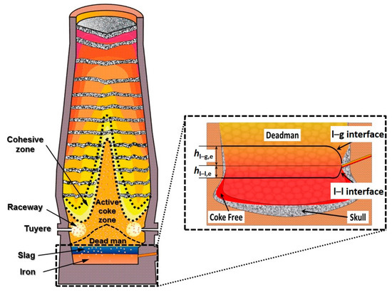
Figure 1.
Schematic vertical cross-section of the blast furnace. l–g interface: slag–gas interface; l–l interface: slag–iron interface; hl–l,e: final level of the horizontal part of the l–l interface; hl–g,e: final level of the horizontal part of the l–g interface.
Due to the importance and complexity of the behavior of the interfaces, many studies of the interface phenomena in the hearth have been done in small-scale experimental models and using sophisticated numerical simulation models. Tanzil et al. [3,4,5] were the first to shed light on the general motion and bending of the interfaces in the BF hearth during drainage, partly revising the findings of Fukutake and Okabe [13]. Detailed investigations of the interface phenomena have been conducted based on the general findings by Tanzil et al. [3,4,5] and by Zulli [6]. Researchers have established simplified mathematical models estimating the l–l and l–g interface levels in the BF hearth as offline tools [10,11,12,14] or online based on measurement data [15,16]. Efforts have also been made to study the sophisticated interface phenomena by Computational Fluid Dynamics (CFD) [17] or a combination of this technique with the Discrete Element Method (CFD–DEM) [18,19,20]. Even though there are many merits of numerical simulation, e.g., low economic cost, high efficiency, etc., experimental studies are still critically essential for verification of numerical models and for studying certain phenomena for which computational analysis is still cumbersome. Experiments studying the effect of operation conditions, such as coke-free zones, hearth coke permeability, etc., on the behavior of the interfaces in batch or continuously operated small-scale physical models have been reported [3,4,5,6,8,9,11]. Compared with simulation studies, the experimental investigations are far more laborious, both when it comes to undertaking the experiments and when analyzing and compiling the results to yield generic findings. Still, the experimental approach is sometimes justified as it studies the “real” system, albeit in a simplified form.
In order to gain a better view of the complex evolution of the liquid levels in the blast furnace hearth, a series of experiments has been conducted in a two-dimensional Hele–Shaw (H–S) model; this kind of viscous flow analog model of the conditions in the BF hearth was used extensively in the pioneering studies in Australia [3,4,5,6,8]. The present work was primarily aimed at a systematical investigation of the effect of operation parameters such as the initial amount of iron and slag, slag viscosity, and blast pressure on the gas breakthrough time, as well as the interface states at the termination of drainage. In practice, the permeability of the packed bed also affects the drainage process, but this factor was constant here because the spacing between the plates in the pilot model was fixed. Pictures taken by a high-speed camera during the experiments were interpreted by an automatic interface tracking program to determine both the l–l and l–g interfaces accurately during the draining process, and the results will be described in this paper. The section that follows describes the apparatus arrangement and procedure as well as experimental conditions and analytical methods. Section 3 presents the results of the experiments that are analyzed and illustrated in both dimensional and dimensionless forms. Finally, in Section 4 some conclusions are drawn on the basis of the results of the study.
2. Experimental Setup
2.1. Apparatus Arrangement and Procedure
The experimental apparatus, as shown in Figure 2, consisted of three main subsystems, i.e., the draining system, charging system, and recording system. The draining system included an H–S model and a liquid receiver. The H–S model consisted of two parallel Perspex plates (585-mm wide and 580-mm high) which were kept at a uniform distance of 2 mm by Perspex strips along the bottom and sidewalls and a number of mini-spacers inside of the model. Three ports were cut in the two sides of the H–S model to allow for fluid supply or extraction. One of the ports, the outlet, was connected by a hose to a liquid receiver that was held at vacuum pressure by a pump to which it is connected. The volume of the receiver was large enough to keep the vacuum pressure practically constant during the draining process, so the pressure was set prior to the experiment. Oil and water were used as the fluids in the study, while the upper part of the model was open, so atmospheric pressure prevailed at the upper oil surface in the experiments. The oil supply system consisted of a moveable oil distributor, an oil reservoir, and a variable-speed peristaltic pump. The moveable oil distributor included of a rectangular mini-container connected to a group of tiny tubes. The container was connected to an oil reservoir by a hose with a variable-speed peristaltic pump. During the oil charging process, the tiny tubes were introduced into the slot of the H–S model, reaching down to the +120 mm level with reference to the outlet. This arrangement was necessary to be able to create a uniform and horizontal oil layer in a relatively short time, after which the pipes were withdrawn and the mini-container was removed (so as not to interfere with the images). The water charging system was very simple since the water supply could be controlled easily: a tube was connected from a water reservoir to the water inlet of the model and the flow rate was adjusted manually using a ball valve. A lifting table was used to support the oil and water reservoirs at a relatively high level for injecting water and oil into the model by gravity. The water supply rate was controlled by adjusting the height of the lifting table and the opening of the ball valve. The supplementary system (i.e., recording system) was a combination of a high-speed camera and laptop, which was used to record the whole drainage process of the experiment. By using the high-speed camera, the starting and terminal points of the drainage process could be determined accurately and more details about the drainage phenomena could be efficiently captured.
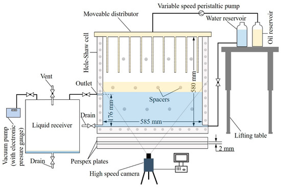
Figure 2.
Schematic illustration of the experimental setup.
As the core part of the apparatus, the H–S viscous flow model emulates the two-phase flow in the BF hearth (i.e., the flow of molten iron and slag) by using mineral oil and water in the model. The approach is based on a flow analogue between viscous liquid flow between two closely parallel plates and flow in a packed bed [4]. Using the H–S model instead of a packed bed model solves the flow visualization problem. The physical properties of the above fluids are reported in Table 1.

Table 1.
Physical properties of fluids for the blast furnace (BF) and model system.
According to the viscous flow analogue, Darcy flow in a packed bed with hydraulic conductivity, K, can be described with the H–S model (as explained in detail in [4]), if
where is the spacing between the plates in the H–S model, g is the gravitational acceleration, is the liquid viscosity, and is the liquid density.
The definition of hydraulic conductivity in a packed bed model is
where k is the absolute permeability of the packed bed. Combining the two equations above, we obtain
In the experiments, the oil and water flow through the H–S model emulates iron and slag flow in the BF hearth, so
Since the fluids in the BF hearth and in the experimental model show practically equal density-to-viscosity ratios, a relation between the plate spacing, b, and the absolute permeability of the packed bed is obtained as
Thus, by adjusting the space of two plates in the H–S model, it is possible to simulate the iron and slag flow in the dead man with a wide range of absolute permeability for the H–S model (although the ratio of hydraulic conductivities of the two liquids remains unchanged). In the BF hearth, a typical effective coke particle diameter is 35 mm and the porosity is 0.30–0.40. According to the empirical relationship between effective particle diameter and absolute permeability [21], a rough estimate of the permeability is k ≈ 10−7 m2. By choosing b 2 mm, the absolute permeability of the BF hearth coke bed can be simulated by the H–S model.
The experimental procedure includes the following main steps:
- (1)
- The lifting table was elevated to a certain level, followed by opening the ball valve to charge water into the model until the predetermined level was reached.
- (2)
- The moveable oil distributor was fixed on top of the model and the peristaltic pump was started at low pumping speed to feed oil into the model slowly to create an oil layer with uniform and desired thickness.
- (3)
- A settling time of a few minutes was allowed for both l–g and l–l interfaces to become absolutely stable. After this, the oil distributor was removed from the top of the model.
- (4)
- The vacuum pump was switched on until the desired under-pressure was obtained in the receiver.
- (5)
- The high-speed camera was turned on to record the drainage process.
- (6)
- The outlet was opened fully. When air started blowing out through the outlet, the outlet was closed and the camera was switched off.
- (7)
- The vent was opened to recover the receiver pressure, and the drain of the receiver was opened to empty the receiver.
2.2. Experimental Conditions and Analytical Methods
For the industrial BF, before the start of tapping, the blast pressure, l–l and l–g interface levels, and slag viscosity may vary from tap to tap, and all of these conditions influence the drainage of the hearth. Thus, it is interesting to study the influence of the above conditions on the tapping in the experimental model to gain insight into the practical drainage behavior of the BF hearth.
In the experiments, four conditions, i.e., pressure difference, initial l–l interface level, oil viscosity, and initial oil layer thickness, were chosen to investigate the drainage phenomena. The experimental conditions are listed in Table 2. The first group of experiments was the benchmark for the full set of experiments. In the table, the pressure difference is the difference between atmospheric pressure (that acts on the l–g interface) and the pressure inside the receiver. The initial l–l interface level, hl-l,0, is expressed with respect to the level of the outlet. In the BF, it depends on the accumulated iron amount in the hearth, and on the length and outer level of taphole, since the true taphole tilts downwards. In the H–S model, it is not convenient to study the effect of the taphole length, so the initial l–l level was directly affected by the amount of water fed into the model. The reported initial oil layer thickness, hoil,0, is the absolute thickness in the model.
Table 2.
Experimental conditions. Changed parameters are written in bold. The dynamic viscosity of water is 0.001 Pa·s for all the experiments.
After each group of experiments, the videos recorded during the drainage process were processed to extract the required information. Since the experimental model was two-dimensional, it was feasible to estimate the remaining volume of oil and water in the model by calculating the oil and water areas in every picture and multiplying them by the spacing between the two plates. A routine was written in MATLAB R2018a (by The MathWorks, MA, USA) to automatically detect the l–l and l–g interfaces to determine the interface locations. Then the areas of both liquids and finally the residual volume could be easily determined for every frame of the video. The method for automatic interface detection and processing is described elsewhere [22]. Figure 3 illustrates schematically the initial and end states of a hypothetical case.
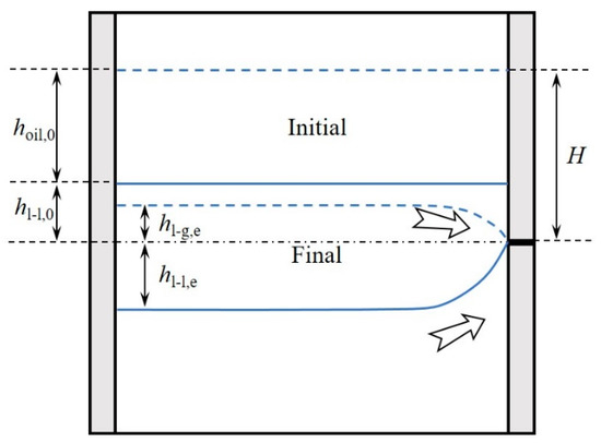
Figure 3.
Schematic illustration of initial and final interface states. Solid lines: l–l interface, Dashed lines: l–g interface.
To use the experimental results for a real BF, some results were dealt with in a dimensionless format, i.e., the residual oil (or water) ratio (α), dimensionless gas breakthrough time (τ), and flow-out coefficient (FL), where the last factor is an important dimensionless variable characterizing the drainage [6]. The definitions of the above parameters are
where Vstart and Vend are the total oil or water volume at the start and end of drainage, respectively. In the equations, D is the width of the H–S model, t is the gas breakthrough time, and tave is the time taken to drain the whole liquids above the outlet at the average tapping rate, Q. Furthermore, hl-l,0 is the initial level of the l–l interface above the outlet, hoil,0 is the initial absolute oil layer thickness in the model, is the shape factor of coke particles, ε is the bed porosity, d is the particle diameter, μ is the viscosity and ρ the density of oil, is the superficial velocity, k is the absolute permeability of coke bed in hearth, and H is the initial level of l–g interface above the outlet.
3. Results and Discussion
In order to provide a general view of the evolution of the interfaces, Figure 4 shows an example of the liquid levels detected at five different moments during the process of a draining experiment. The figure shows how the l–g interface (blue line) from being horizontal gradually bends downwards towards the outlet along with the progress of the draining, while, by contrast, the l–l interface starts bending upwards after the interface in question has reached the level of the outlet. It is also seen that the l–g interface bends more than the l–l interface, which is due to differences in viscosity and density of the two liquid phases.
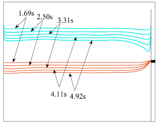
Figure 4.
Interfaces between oil and gas (l–g, blue lines) and water and oil (l–l, red lines) at five different moments during a draining experiment.
3.1. Influence on Residual Ratio, Tapping Time
For the BF operation, the residual ratio of both liquids and tapping time are critical parameters. Under certain conditions, a longer tapping time may mean a higher operation rate and lower economic costs, because with extended tapping the residual liquid ratios and frequency of drilling and plugging of the taphole decrease, thereby reducing the cost of refractory materials and taphole clay.
3.1.1. Influence of Initial Oil Layer Thickness
In the BF, the amount of molten slag depends on the grade of iron ore, quality of coke, and the amount of injected pulverized coal, so it may fluctuate with the quality and quantity of raw materials used. If the slag ratio (i.e., the ratio of produced slag and hot metal) is high, the accumulated slag layer is thicker and there is more slag in the BF hearth during the drainage. To study the influence of the thickness of the accumulated slag layer on the tapping, a group of experiments was conducted, with results shown in Figure 5, where the experiments acted as benchmarks.
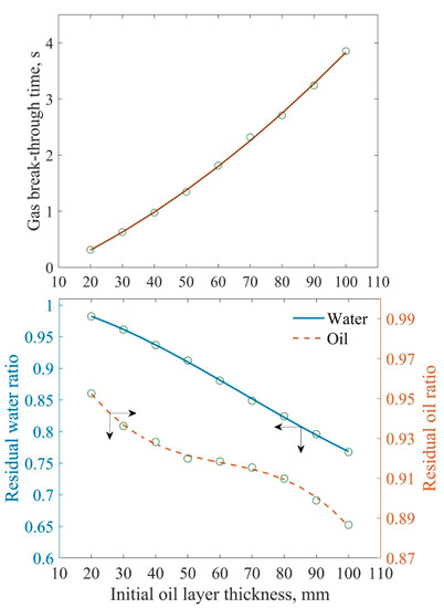
Figure 5.
Upper panel: Effect of initial oil layer thickness on gas breakthrough time. Lower panel: Effect of initial oil layer thickness on residual ratios of both liquids. Initial l–l interface 10 mm above the outlet, with a pressure difference of 0.3 bar and oil viscosity of 0.131 Pa·s (cf. Table 2).
The upper panel of the figure shows that, as expected, the draining time increased with the initial oil layer thickness. This is simply because the distance between outlet and l–g interface increased since the initial l–l interface level was kept constant. The lower panel of the figure illustrates that both residual liquid ratios decreased with the initial oil layer thickness and that the decrease of the residual water ratio was more significant. The primary reason for the lower water residual ratio was that the thicker initial oil layer delayed the moment when the oil surface bent downwards to the outlet, which was the end point of the drainage, and the l–l interface thus had longer time to descend. This is also the reason why the residual oil ratio was smaller, as illustrated in the schematic in Figure 6; even though the water level is lower, the residual oil ratio decreased as the end l–g level increased only slightly.
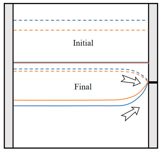
Figure 6.
Schematic of initial and final interface states for two initial oil layers enclosed by blue and orange lines. Solid lines: l–l interface, Dashed lines: l–g interface.
Thus, for the BF process, with less produced slag, the draining time would be shorter. As this would lead to more frequent taps, implying higher labor and refractory costs, it is necessary to decrease the taphole diameter to extend the draining time in such situations.
3.1.2. Influence of the Initial l–l Interface Level
The initial l–l interface level (above the taphole) is related to the amount of accumulated molten iron in the BF hearth at the commencement of drainage, the dead man porosity, the level of the taphole, and the taphole length. For multi-taphole furnaces, it is also strongly related to the operation of the alternate taphole used [10,12]. The outer level of the taphole is predetermined for every BF, but the angle and the length of the taphole may vary. Even though the former is usually fixed, it is known that some plants used the taphole angle for controlling the drainage. As for the taphole length, it is a controllable factor (under favorable conditions [23]), as it can be adjusted by injecting more or less taphole clay during taphole plugging.
A group of experiments was undertaken to investigate the effect of the initial l–l interface. Figure 7, which illustrates the results, shows how the gas breakthrough time increased with the level of the initial l–l interface at a fixed initial oil layer thickness. This is natural since a higher initial water level delays the moment when oil starts flowing out. The lower panel of the figure shows that both the residual water and oil ratios decreased as the initial l–l interface rose. The reason is that an overall increase in the initial l–l level yields a longer drainage time and therefore lowers residual amounts of the two liquids.
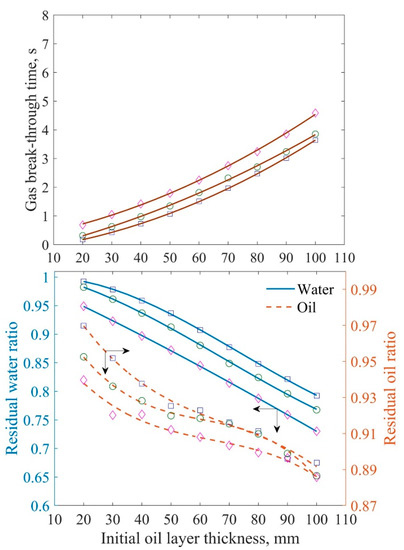
Figure 7.
Upper panel: Effect of initial oil layer thickness on gas breakthrough time at different initial l–l interface levels. Lower panel: Effect of initial oil layer thickness on residual ratios of both liquids at different initial l–l interface levels. Pressure difference: 0.3 bar, oil viscosity: 0.131 Pa·s, initial l–l interface levels: 5 mm (marked by squares), 10 mm (marked by circles), and 20 mm (marked by diamonds).
3.1.3. Influence of Pressure Difference
The blast pressure of an operating BF is usually kept relatively stable, which means that the difference between the internal pressure and the atmospheric pressure is constant. However, the pressure difference varies with the blast volume and can also be adjusted by changing the BF top pressure. To clarify the effect of this “driving force”, the pressure difference in the experimental system was varied. The results for different oil layer thicknesses are reported in Figure 8, where the upper panel shows that the draining time decreased dramatically with the pressure difference (at fixed initial oil layer thickness and initial l–l level). The obvious reason is that the outflow rates of both liquids increased with the pressure difference. The decrease of the tapping time was more pronounced at a thicker initial oil layer. When the initial oil layer was thin, water was the dominant phase to be drained during the whole drainage period but along with the increase in the initial oil layer thickness, the ratio of water to oil in the outflow decreased, particularly in the later stages of the process. When the initial oil layer was thicker, the tapping time increased significantly due to the overall higher drainage resistance. The lower panel of Figure 8 shows that both residual liquid ratios increase with the increase in pressure difference at a fixed initial amount of water and oil. This was presumably caused by the fact that a higher pressure proportionally increases the draining rate of oil more than that of water, implying an earlier end point of the draining. Thus, a lower pressure difference (i.e., a lower blast pressure) was beneficial for extending the draining time and decreasing the residual liquid ratios. However, in the BF a certain blast pressure is needed for a normal operation of the process to support the burden and to suppress undesired gasification reactions and fluidization.
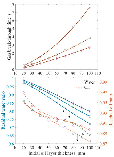
Figure 8.
Upper panel: Effect of initial oil layer thickness on gas breakthrough time at different pressure differences. Lower panel: Effect of dimensionless initial oil layer thickness on residual ratios of both liquids at different pressure differences. Initial l–l interface level: 10 mm, oil viscosity: 0.131 Pa·s, pressure differences: 0.2 bar (squares), 0.3 bar (circles), and 0.4 bar (diamonds).
3.1.4. Influence of Oil Viscosity
The slag viscosity mainly depends on temperature and composition, but also on the contents and characteristics of possible solid components (e.g., char). The temperature varies with the thermal state of the process, while the slag composition depends on the type and quantity of raw materials used, and thus it may vary with time. The slag composition is also affected by the partition reactions between iron and slag, which are influenced by the temperature. Figure 9 illustrates the role of oil viscosity on the gas breakthrough time and residual ratios. The tapping time grew with the oil viscosity since the draining rate became lower. With the increase in oil viscosity, the declivity of the l–g interface near the taphole should grow because of an increased pressure drop in the oil phase, but the videos from the experiments showed little change in the bending degree of l–g interface near the taphole, so the effect of draining rate was dominant for this group of experiments. Thus, as the oil viscosity increased, the tapping time increased almost solely due to a decreased tapping rate.
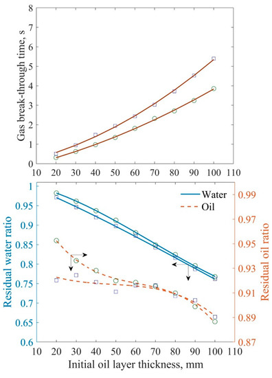
Figure 9.
Upper panel: Effect of initial oil layer thickness on gas breakthrough time at different oil viscosities. Lower panel: Effect of initial oil layer thickness on residual ratios of both liquids at different oil viscosities. Initial l–l interface level: 10 mm, pressure difference: 0.3 bar, oil viscosity: 0.131 Pa·s (circles), 0.254 Pa·s (squares).
The lower panel of Figure 9 shows that the residual water and oil ratios decreased with an increase in oil viscosity, which is mainly because of the extension of draining time. The results indicate that high slag viscosity may extend draining time, but the high draining resistance and low tapping rate could in practice cause drainage difficulties with an adverse effect on the stability of the hearth operation.
3.2. Effect of the Factors on the End State
In the draining experiments, three different types of end states occurred, here labelled abnormal drainage, transitional drainage, and normal drainage, respectively. These are illustrated in Figure 10 for three draining experiments using the parameters of experimental group 1, i.e., an initial l–l level of 10 mm, a pressure drop of 0.3 bar, and an oil viscosity of 0.131 Pa·s, but different initial oil layer thicknesses. The horizontal blue line in the figure represents the level of the outlet. In the first type of drainage (top panel, 20 mm initial oil layer), the conditions were such that the overall water level did not even descend to the outlet level but was slightly above it at the point when air broke out. This pattern primarily occurred when the initial oil layer was thin. By contrast, in the final type, i.e., normal drainage (bottom panel, 70 mm initial oil layer), the l–l interface descended clearly below the outlet in the final state and thus bent upwards to the outlet. The cases referred to as transitional represent drainage patterns that fell between these two extremes (middle panel, 40-mm initial oil layer), where the l–l interface was practically horizontal and its vertical level was very close to the outlet level when the drainage ended. It may be noted that this pattern could also occur for a case with a thin initial oil level and an initial l–l interface at the taphole (not studied in the present investigation).
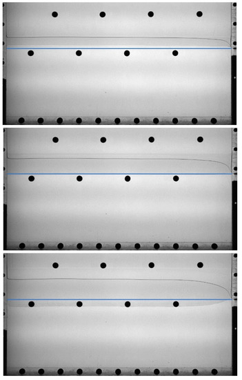
Figure 10.
Interface levels at the termination of drainage for abnormal drainage (top panel), transitional drainage (middle panel), and normal drainage (bottom panel) in three experiments with an initial l–l interface level of 10 mm, a pressure drop of 0.3 bar, and oil viscosity of 0.131 Pa·s. The initial oil layer thicknesses are 20 mm, 40 mm, and 70 mm (top to bottom panels).
In order to gain an understanding of the state of the end interfaces, some experiments will be illustrated, showing the influence of the initial oil layer thickness, initial l–l interface level, pressure difference, and oil viscosity. The drainage was studied for different initial oil layer thicknesses. In every group, it was observed that abnormal drainage occurred if the initial oil layer was thin, but with the increase of the oil layer thickness the drainage type evolved gradually through the transition to the normal drainage patterns, as shown in Figure 11. Thus, for each case, there is an initial oil thickness, henceforth called the “critical oil layer thickness”, for which the drainage ends with an l–l interface at the taphole. If the initial thickness exceeds the critical value, normal drainage will occur. Thus, for a case with large critical oil layer thickness, abnormal drainage is more likely to occur than for a case with small critical oil layer thickness. To study the effect in more detail, some more experiments were conducted and the end levels of the horizontal part of both interfaces were determined, with results shown in Table 3. The end state is reported as the final level of the horizontal part of the l–l interface, hl-l,e. The conditions for abnormal, transitional, and normal drainage applied were hl-l,e > 1 mm, 1 ≥ hl-l,e ≥ −1 mm, hl-l,e < −1 mm, respectively.
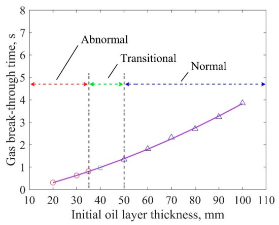
Figure 11.
Effect of initial oil layer thickness on the drainage end state. Initial l–l interface level: 10 mm, pressure drop: 0.3 bar, oil viscosity: 0.131 Pa·s.
Table 3.
Levels of horizontal parts of the interfaces at the end of drainage under different experimental conditions (cf. Table 2). Values that fall in the transition zone have been indicated by bold values, and lack of experimental results by an em dash (—).
3.2.1. Effect of the Initial l–l Interface Level
The effect of the initial l–l interface level on the drainage type is presented in dimensional and dimensionless form in Figure 12, demonstrating that the critical oil layer thickness increased and the corresponding flow-out coefficient decreased with the initial l–l interface level. For the purpose of clarity, dashed red lines were drawn through the observations that represent the transitional drainage. A possible explanation for the increase in the critical oil layer thickness is that with the rise of the initial l–l interface, the initial outflow rate of water increases since water occupies the regions above and below the outlet, which makes the oil layer more prone to bend when the oil outflow commences.
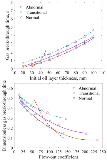
Figure 12.
Effect of initial l–l interface level on the drainage end state. Pressure difference: 0.3 bar, oil viscosity: 0.131 Pa·s, initial l–l interface levels: 5 mm (dash-dotted line), 10 mm (solid line), 20 mm (dashed line). Red dashed line shows the states corresponding to transitional drainage.
3.2.2. Effect of the Pressure Difference
The effect of the pressure difference on the end state is illustrated in Figure 13, which shows that the critical oil layer thickness increased with the imposed pressure difference. As the driving force for both water and oil transport increased, the draining rates of both liquids increased, raising the descending speed of the l–l and l–g interfaces. The higher oil draining rate also increased the bending of the l–g interface at the outlet, leading to a decrease in the gas breakthrough time. Consequently, the critical oil layer thickness increased. The lower panel of Figure 13 shows that the flow-out coefficient corresponding to the critical oil layer thickness was rather insensitive to the pressure difference.
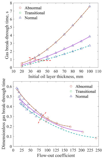
Figure 13.
Effect of pressure difference on the drainage end state. Initial l–l interface level: 10 mm, oil viscosity: 0.131 Pa·s, pressure differences: 0.2 bar (dash-dotted line), 0.3 bar (solid line), 0.4 bar (dashed line).
3.2.3. Effect of Oil Viscosity
Finally, Figure 14 illustrates the role of oil viscosity on the drainage type, showing that the critical oil layer thickness decreased and the corresponding flow-out coefficient increased with the oil viscosity. The reason for the decrease of the critical oil layer thickness is that the increased oil viscosity made this phase flow out at a much lower speed, making it less likely that the drainage would end before the water level descended below the taphole.
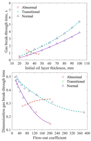
Figure 14.
Effect of oil viscosity on the drainage end state. Initial l–l interface level: 10 mm, pressure difference: 0.3 bar, oil viscosity: 0.131 Pa·s (solid line), 0.254 Pa·s (dashed line).
3.3. Comparison with Earlier Findings
To allow for a comparison of the results of the present work with earlier findings by other authors, the residual oil ratios were re-calculated according the definition applied by Tanzil et al. [4,5], i.e., as the ratio of the volume of liquid (slag) remaining above the taphole level at the termination of the drainage to the volume originally above the taphole. Using this definition, the residual oil ratios in the experiments of the present work are depicted in Figure 15. The ratio is seen to increase quite linearly with the logarithm of the flow-out coefficient but levels out at high values. The overall trend is in accordance with that presented by Tanzil and co-workers (e.g., Figure 4 of [4]) even though the flow-out coefficient of the present work is higher, caused by the different experimental conditions (e.g., liquid properties).
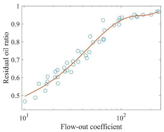
Figure 15.
Effect of the flow-out coefficient on the residual oil ratio re-calculated according to the definition in [4,5].
Figure 16 provides a comparison with some other results reported by earlier investigators. The left panels show findings reproduced from He et al. [9] who used a packed bed model in their research, while the right panels are compiled results from the present research for a pressure drop of 0.3 bar and an oil viscosity of 0.131 Pa·s. The different experimental set-up and conditions (fluids, pressure drop) in the two systems make the absolute values of the variables different, so the focus should rather be on trends in the comparison. The upper panels show how the gas break-out time varies with the initial level of the l–g interface. He et al. started the experiments with the l–l interface below (–20 mm), at (0 mm), or above (+20 mm) the outlet, while the experiments of this paper were started above (+5 mm, +10 mm, and +20 mm) the outlet. As observed by He et al., there is a slightly superlinear relation of the gas breakthrough time to the initial l–g level. In contrast to He’s results, the present work shows little effect of the initial l–l level. One would, in fact, expect the initial l–l level to have a lowering effect on the drainage time since the drainage is faster if a higher share of the drained liquids is the less viscous one. The differences in drainage time between the experiments with different initial l–l levels are, however, so small that stochastic effects may mask these.
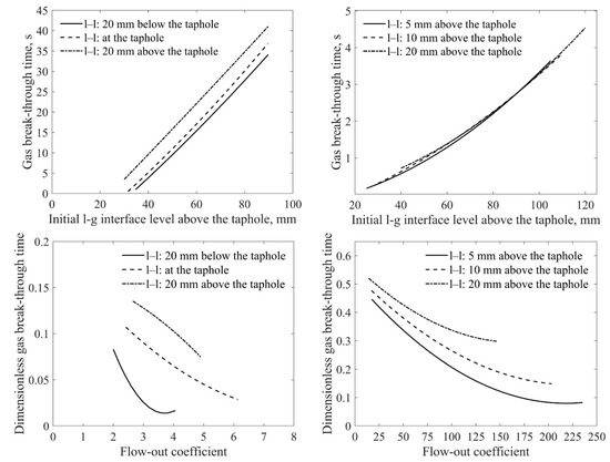
Figure 16.
Comparison of some results from He et al. [9] (left panels) with results of the present work (right panels). Top: Effect of initial l–g interface on gas breakthrough time. Bottom: Effect of flow-out coefficient on dimensionless gas breakthrough time.
The lower panels depict how the dimensionless breakthrough time (cf. Equation (8)) depends on the flow-out coefficient. Again, even though the magnitudes of the variables are different, the overall trend exhibited by them can be concluded to coincide well.
4. Conclusions
In order to gain a better understanding of the drainage and evolution of the liquid–gas and liquid–liquid interfaces in the blast furnace hearth, a series of experiments were conducted with a two-dimensional Hele–Shaw model. Oil and water were used as the two liquids emulating slag and iron in the real system. Special attention was focused on the effect of the conditions on the gas breakthrough time, residual ratios of both liquids, and the end state of the liquid levels, categorized into three groups (normal, transitional, or abnormal drainage). Based on the experimental results, the following conclusions can be drawn:
- (1)
- An increase in the initial oil layer thickness (i.e., more accumulated slag in the hearth) extends the draining time and decreases the residual ratios of both liquids. In addition, the likelihood of abnormal drainage also decreases.
- (2)
- With a higher initial l–l interface level, the draining time increases and the residual liquid ratios decrease. The likelihood of abnormal drainage increases.
- (3)
- With an increased pressure difference (“driving force”) in the system, the residual liquids ratios and the likelihood of abnormal drainage increase, while the gas breakthrough time decreases.
- (4)
- An increase of oil viscosity increases the tapping time and reduces the likelihood of abnormal drainage and residual ratios of both liquids.
The findings can be used to provide a better interpretation of the drainage patterns observed in the blast furnace, and the results may further be applied to calibrate and verify computational fluid dynamics models of the blast furnace hearth.
Author Contributions
Conceptualization, W.L. and L.S.; Data curation, W.L. and L.S.; Formal analysis, W.L. and H.S.; Funding acquisition, H.S.; Investigation, W.L. and L.S.; Methodology, W.L. and L.S.; Project administration, H.S.; Resources, H.S.; Software, W.L.; Supervision, H.S. and L.S.; Writing—original draft, W.L.; Writing—review and editing, H.S. All authors have read and agreed to the published version of the manuscript
Funding
This research was funded by National Natural Science Foundation of China (Grant 51604068) and Åbo Akademi Foundation.
Acknowledgments
This work was carried out with support from the Åbo Akademi Foundation, and this funding is gratefully acknowledged. The second author (Lei Shao) wishes to thank the National Natural Science Foundation of China (Grant 51604068) for providing financial support for this work.
Conflicts of Interest
The authors declare no conflict of interest.
References
- Geerdes, M.; Toxopeus, H.; vd Vliet, C. Modern Blast Furnace Ironmaking: An Introduction, 2nd ed.; IOS Press BV: Amsterdam, The Netherlands, 2009. [Google Scholar]
- Brännbacka, J. Model Analysis of Dead-Man Floating State and Liquid Levels in the Blast Furnace Hearth. Ph.D. Thesis, Åbo Akademi University, Turku, Finland, 2004. [Google Scholar]
- Pinczewski, W.V.; Tanzil, W.B.U.; Hoschke, M.I.; Burgess, J.M. Simulation of the drainage of two liquids from a blast furnace hearth. Tetsu-to-Hagane 1982, 68, S111. [Google Scholar]
- Tanzil, W.B.U.; Zulli, P.; Burgess, J.M.; Pinczewski, W.V. Experimental model study of the physical mechanisms governing blast furnace hearth drainage. Trans. Iron Steel Inst. Jpn. 1984, 24, 197–205. [Google Scholar] [CrossRef]
- Tanzil, W.B.U. Blast Furnace Hearth Drainage. Ph.D. Thesis, University of New South Wales, Sydney, Australia, 1985. [Google Scholar]
- Zulli, P. Blast Furnace Hearth Drainage with and without a Coke-Free Layer. Ph.D. Thesis, University of New South Wales, Sydney, Australia, 1991. [Google Scholar]
- Shao, L.; Saxén, H. Simulation study of blast furnace drainage using a two-fluid model. Ind. Eng. Chem. Res. 2013, 52, 5479–5488. [Google Scholar] [CrossRef]
- He, Q.; Zulli, P.; Evans, G.M.; Tanzil, F. Free surface instability and gas entrainment during blast furnace drainage. Dev. Chem. Eng. Miner. Process. 2006, 14, 249–258. [Google Scholar] [CrossRef]
- He, Q.; Evans, G.; Zulli, P.; Tanzil, F. Cold model study of blast gas discharge from the taphole during the blast furnace hearth drainage. ISIJ Int. 2012, 52, 774–778. [Google Scholar] [CrossRef]
- Iida, M.; Ogura, K.; Hakone, T. Analysis of drainage rate variation of molten iron and slag from blast furnace during tapping. ISIJ Int. 2008, 48, 412–419. [Google Scholar] [CrossRef]
- Nouchi, T.; Yasui, M.; Takeda, K. Effects of particle free space on hearth drainage efficiency. ISIJ Int. 2003, 43, 175–180. [Google Scholar] [CrossRef]
- Roche, M.; Helle, M.; van der Stel, J.; Louwerse, G.; Shao, L.; Saxén, H. Off-line model of blast furnace liquid levels. ISIJ Int. 2018, 58, 2236–2245. [Google Scholar] [CrossRef]
- Fukutake, T.; Okabe, K. Influences of slag tapping conditions on the amount of residual slag in the blast furnace hearth. Trans. Iron Steel Inst. Jpn. 1976, 16, 317–323. [Google Scholar] [CrossRef]
- Brännbacka, J.; Torrkulla, J.; Saxén, H. Simple simulation model of blast furnace hearth. Ironmak. Steelmak. 2005, 32, 479–486. [Google Scholar] [CrossRef]
- Brännbacka, J.; Saxén, H. Modeling the liquid levels in the blast furnace hearth. ISIJ Int. 2001, 41, 1131–1138. [Google Scholar] [CrossRef]
- Roche, M.; Helle, M.; van der Stel, J.; Louwerse, G.; Shao, L.; Saxén, H. On-line estimation of liquid levels in the blast furnace hearth. Steel Res. Int. 2019, 90, 1800420. [Google Scholar] [CrossRef]
- Nishioka, K.; Maeda, T.; Shimizu, M. Effect of various in-furnace conditions on blast furnace hearth drainage. ISIJ Int. 2005, 45, 1496–1505. [Google Scholar] [CrossRef]
- Zhou, Z.; Zhu, H.; Yu, A.; Zulli, P. Numerical investigation of the transient multiphase flow in an ironmaking blast furnace. ISIJ Int. 2010, 50, 515–523. [Google Scholar] [CrossRef]
- Vångö, M.; Pirker, S.; Lightenegger, T. Unresolved CFD–DEM modeling of multiphase flow in densely packed particle beds. Appl. Math. Model. 2018, 56, 501–516. [Google Scholar] [CrossRef]
- Bambauer, F.; Wirtz, S.; Sherer, V.; Bartusch, H. Transient DEM-CFD simulation of solid and fluid flow in a three dimensional blast furnace model. Powder Technol. 2018, 334, 53–64. [Google Scholar] [CrossRef]
- Bear, J. Dynamics of Fluids in Porous Media, 1st ed.; American Elsevier Company: New York, NY, USA, 1972; p. 133. [Google Scholar]
- Liu, W.; Mondal, D.N.; Shao, L.; Saxén, H. An image analysis-based method for automatic data extraction from pilot draining experiments. Ironmak. Steelmak 2020. submitted manuscript. [Google Scholar]
- Tsuchiya, N.; Fukutake, T.; Yamauchi, Y.; Matsumoto, T. In-furnace conditions as prerequisites for proper use and design of Mud to control blast furnace taphole length. ISIJ Int. 1998, 38, 116–125. [Google Scholar] [CrossRef]


© 2020 by the authors. Licensee MDPI, Basel, Switzerland. This article is an open access article distributed under the terms and conditions of the Creative Commons Attribution (CC BY) license (http://creativecommons.org/licenses/by/4.0/).