Transient Simulation of Bath Temperature inside Aluminum Reduction Cells

Abstract

Bath temperature stability is a very important parameter with which to evaluate pot thermal balance. In this paper, a transient thermo-electric finite element model of reduction cell is established to simulate the fluctuation curve of bath temperature under different alumina feeding rates and different energy inputs. The model results show that short-term fluctuation of the temperature curve is influenced by different alumina feeding rate under underfeeding and overfeeding, but the long-term fluctuation depends on whether energy input matches average feeding rate. If the difference between energy input and heat consumed by alumina reaches the latter’s 10%, the temperature changes about 1.8 °C after four cycles. Based on model results, the paper analyzes the relationship among alumina feeding rate, bath temperature fluctuation and heat balance. The matching of heat input and heat consumed by alumina is of crucial importance to maintaining bath temperature stability.

1. Introduction

Pot heat balance is necessarily paid much attention during a pot’s operation, which mainly involves maintaining a stable bath temperature, a proper superheat range, a good ledge, etc. Much research [1,2,3,4,5] shows that heat balance is the key factor to maintaining high efficiency and low energy consumption by the pot.

A few researchers have done transient simulations of aluminum electrolysis bath temperature. Taylor [6] studied the dynamics and performance of an electrolysis bath, and illustrated the impact of alumina dissolution on the electrolyte temperature. The addition of alumina had the most energy-intensive influence on electrolyte temperature. Alumina feeding gave rise to a drastic but temporary decrease in electrolyte temperature and superheating. Ding [7] did a simulation study on the change of bath temperature during alumina feeding, and the results showed that the alumina feeding had a great influence on the transient bath temperature’s fluctuation.

Some researchers have studied the influence [8,9,10,11] of alumina feeding on bath temperature and heat balance. Thonstad [8] believed that the alumina dissolution was firstly controlled by the heat transfer, and then by the mass transfer. Therefore, the superheat is of great importance to the alumina dissolution. Thomas [9] used numerical simulation models to study the dissolution process of alumina particles. Kobbeltvedt [12] measured bath temperature during alumina feeding, and the results showed how the alumina was transported from the feeding position to the rest zone. Kobbeltvedt’s [12] study indicated that alumina dissolution were greatly impacted by the bath flow from underneath the anodes.

Lavoie [13] reviewed 4-step process of alumina dissolution and the impacts of many factors on them, and presented a mechanism for rapid alumina dissolution in an industrial cell. His study indicated that the feeder hole’s condition may have a strong effect on the alumina dissolution. An open feeder hole and sufficient flow velocity together can greatly increase the contact surface between alumina and the liquid bath; furthermore, enough superheat can quickly melt the frozen bath layer around the alumina particles, and thus rapid alumina dissolution occurs.

In aluminum reduction production, technicians will measure the bath’s transient temperature one to two times a day. Since the feeding rates during underfeeding and overfeeding are different, the bath temperature will fluctuate. The temperatures measured at the end of underfeeding period and at the end of the overfeeding period may vary considerably [14]. This temperature deviation caused by different feeding rates may result in improper assessment of the heat balance, meaning the measurement during the normal feeding period can reduce improper assessment. It is quite difficult to take all manual measurements on many pots during normal feeding, and it may take more time. However, an intermittent, online, automatic temperature measurement system can easily realize measurement during normal feeding; therefore, online measurement of process parameters to diagnose pot status will become a trend in the future [14,15].

Intermittent online measurement can acquire temperature data for consecutive minutes each time. Research into the influence of the feeding interval on the bath temperature should provide a basis for the future processing of online bfigureath temperature measurements, and should also provide guidance for setting one’s feeding interval system. In this paper, a computational finite element simulation is used to compare and study the corresponding change trends and rules of bath temperature under various feeding interval systems and energy input conditions.

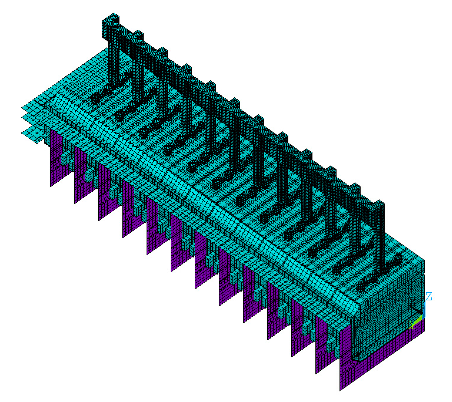
2. Finite Element Simulation Model

This paper focuses on a 500 kA pot in an aluminum smelter, adopts ANSYS finite element software for simulation and establishes the transient thermo-electric finite element simulation model.

2.1. Model Simplification and Assumptions

In order to make it simple, the model is established with the following assumptions:

(1).

There is no crust or sludge in the molten aluminum.

(2).

Both the superheat and flow rate are sufficient such that alumina can be completely dissolved without sediments.

(3).

No influences of other operations are considered. Parameters of the aluminum reduction cell for modeling are listed in

Table 1. Parameters of the aluminum reduction cell.

Current/kA	Bath Level/mm	Metal Level/mm	ACD/mm	Numbers of Anode	Anode Size/mm	Anode Raphe/mm	Cathode Size/mm
500	180	300	45	48	1850 × 700 × 620	200	3790 × 720 × 530

.

2.2. Control Equation

Finite element simulation is established based on solving differential equations of a physical process. Most of heat in the pot is generated during current passing the pot and then diffused externally through conduction, convection and radiation.

Differential equation of the 3D electricity conduction process:

$$\nabla \cdot J+\frac{\partial p}{\partial t}=0,J=\sigma \cdot E,E=-\nabla U,p=-\nabla \cdot (\varphi \nabla U)$$

(1)

where

• J is the current density, A·m⁻²;
• E is the electrical field, V·m⁻¹;
• U is the electrical potential, V;
• $\sigma$ is the electrical conductivity, Ω⁻¹·m⁻¹, changing along with temperature;
• p is the change density;
• $\varphi$ is the permittivity.

In this paper, we ignore local charging, i.e., p = 0, and obtain the following equation:

$$\frac{\partial }{\partial x}\left({\sigma }_x\frac{\partial U}{\partial x}\right)+\frac{\partial }{\partial y}\left({\sigma }_y\frac{\partial U}{\partial y}\right)+\frac{\partial }{\partial z}\left({\sigma }_z\frac{\partial U}{\partial z}\right)=0$$

(2)

Boundary conditions for the electricity conduction process:

(1) For surface P₁ with known electrical potential U_b:

$$U(x,y,z){|}_{P_1}=U_b(x,y,z)$$

(3)

(2) For surface P₂ with known current source I:

$$\sigma \frac{\partial V}{\partial n}|{}_{P_2}=-I(x,y,z)$$

(4)

The transient heat transfer differential equation of a 3D object is:

$$\frac{\partial }{\partial x}\left(k_x\frac{\partial T}{\partial x}\right)+\frac{\partial }{\partial y}\left(k_y\frac{\partial T}{\partial y}\right)+\frac{\partial }{\partial z}\left(k_z\frac{\partial T}{\partial z}\right)+q_S=\rho \hspace{0.17em}c\hspace{0.17em}\frac{\partial T}{\partial \hspace{0.17em}t}$$

(5)

Among which:

• T—Temperature, K;
• t—time, s;
• k_x, k_y, k_z—thermal conductivity, W·m⁻¹K⁻¹;
• q_S—strength of heat source or sink, J/m³, including Joule self-heating power and the other heat generation rate defined in the model.
• ρ—material density, kg/m³;
• c—thermal capacity, W·kg⁻¹K⁻¹.

For the heat source from the Joule self-heating power:

$$q_s=E\cdot J$$

(6)

Boundary conditions for heat transfer process:

(1) For surface S₂ with known heat flux q:

$${k_n\frac{\partial T}{\partial n}|}_{s2}=-q(x,y,z)$$

(7)

where k_n is normal thermal conductivity perpendicular to surface S₂.

(2) There are convection and radiation heat transfer conditions between the pot’s external surface S₃ and the environment:

$$\begin{array}{l}{k_n\frac{\partial T}{\partial n}|}_{s3}=h(T-T_g)+\epsilon C_0(T^4-T_g^4)=h_f(T-T_g)\\ h_f=h+\epsilon C_0(T+T_g)(T^2+T_g{}^2)\end{array}$$

(8)

where h is the heat transfer coefficient of the convection between the surface and the environment, ε is the emissivity of pot external surface, C₀ is Stefan–Boltzmann constant, T_g is the environmental temperature and h_f is the equivalent heat transfer coefficient considering both convection and radiation.

Initial conditions are:

$${T(x,y,z)|}_{t=0}=T_0(x,y,z)$$

(9)

The initial temperature distribution T₀(x,y,z) is calculated from the steady state simulation with the same boundary condition as above.

2.3. Material Properties and Boundary Conditions

In the model, the enthalpy material property of a ledge is set to have non-linear variation along with temperature and steps up at the liquidus temperature. The size of the step is the melting enthalpy, which can be used to simulate ledge solidification and melting phenomena. As fluids, the equivalent heat conductivity (k_e) of the bath and molten aluminum can be calculated through characteristic length (L), flow rate (u), density (ρ) and specific heat capacity (C_p), as shown in the following equation [16].

$$k_e=Lu\rho C_p$$

(10)

According to other researchers’ simulation and measurement studies [17,18,19,20], the average flow rate of bath and molten metal is mostly in range of 0.04–0.16 m/s. A typical average value of 0.1 m/s is applied in this study.

The initial state of the transient model is a stable thermo-electric field. The boundary conditions are as follows:

(1).

Heat convection and radiation boundary conditions are applied on the pot’s external surface. The heat convection coefficient of the pot’s side is 5 w·m⁻¹K⁻¹; that of the anode cover’s surface is 10 w·m⁻¹K⁻¹; and that of the anode butt/rod’s surface is 15 w·m⁻¹K⁻¹.

(2).

Current input conditions are applied on the anode rod’s top.

(3).

Zero potential conditions are applied on the steel bar’s end.

The heating and dissolution process of the room temperature alumina entering the bath is achieved by applying heat generation rate. There are six feeders in the pot, which are numbered 1–6 from the tapping end to the duct end. The feeding interval refers to the interval between two consecutive feedings of the same feeder. Feeders 1, 3 and 5 will feed first, at the same time, and feeders 2, 4 and 6 will feed at the same time after 1/2 a feeding interval; and then, after another 1/2 a feeding interval, feeders 1, 3 and 5 start to feed again at the same time. The cycle repeats for a long time. Each of the six feeders within one feeding interval will feed once. Each feeder has a fixed volume of 1.8 kg, and 2674 kJ [21] will be needed for heating and dissolving 1 kg of alumina.

According to the study by Kuschel and Welch [22], alumina dissolution time decreases with the increases of superheat and flow rate. When superheat is more than 10 °C and flow rate is more than 10 cm/s, the dissolution time is about 20–35 s. Thus, 20 s is almost the minimum time for alumina dissolution. Alumina dissolution has a negative impact on heat balance stability. The shorter the dissolution time, the higher the intensity of the impact. This study assumes the dissolution time is 20 s in order to study the temperature evolution under the highest intensity of impact. Furthermore, dissolution time 20 s is only for alumina dissolving in a local feeding zone, not for spreading it to an entire bath zone.

When one feeder starts to feed, it is necessary to apply a negative heat generation rate P_suck (= –2674 × 1.8/20 = –240.66 kW) to the bath element near this feeder (feeding zone). P_suck is distributed in the feeding zone evenly.

P_feeding is defined as the average power for heating and dissolving alumina within a total period of time.

$$P_{feeding}=\frac{2674\times 6\times 1.8\times N}{t}$$

(11)

where, N refers to feeding count and t means a total period of time (refers to total time for one cycle in

Table 2. Simulation conditions of different cases in the transient model (Cases 1–4).

Feeding Type	Item	Case 1	Case 2	Case 3	Case 4
Under feeding	Last time (s)	600	780	720	1200
	Feeding intervals (s)	150	130	180	150
	Feeding rate (kg/s)	0.072	0.083	0.06	0.072
	Feeding count	4	6	4	8
Over feeding	Last time (s)	600	440	480	1200
	Feeding intervals (s)	100	110	80	100
	Feeding rate (kg/s)	0.108	0.098	0.135	0.108
	Feeding count	6	4	6	12
Total feeding count		10	10	10	20
Pfeeding (kW)		240.66	237.71	240.66	240.66
Pheat /Pfeeding		1	1	1	1
Total time for one cycle (s)		1200	1220	1200	2400

and

Table 3. Simulation conditions of different cases in the transient model (Cases 5–8).

Feeding Type	Item	Case 5	Case 6	Case 7	Case 8
Under feeding	Last time (s)	600	600	600	600
	Feeding intervals (s)	150	130	180	150
	Feeding rate (kg/s)	0.072	0.072	0.072	0.072
	Feeding count	4	4	4	4
Over feeding	Last time (s)	600	600	600	600
	Feeding intervals (s)	100	100	100	100
	Feeding rate (kg/s)	0.108	0.108	0.108	0.108
	Feeding count	6	6	6	6
Total feeding count		10	10	10	10
Pfeeding (kW)		240.66	240.66	240.66	240.66
Pheat/Pfeeding		0.9	0.95	1.05	1.1
Total time for one cycle(s)		1200	1200	1200	1200

).

Increasing bath resistance between the anode and cathode can generate additional constant Joule heat generation rate P_heat (compared with the stable thermo-electric field at initial conditions without negative heat generation rate P_suck). It can provide continuous and uniform heat to compensate for the energy spent in the alumina heating and dissolving. In fact, bath resistivity relates to alumina concentration; i.e., pot voltage increases during underfeeding and pot voltage drops during overfeeding. In the model, average P_heat will be applied for simplification. P_feeding distribution and P_heat distribution in terms of the transient time scale are different; P_feeding refers to pulse consumption of bath internal energy and P_heat supplies continuous and uniform heat.

In order to calculate the bath temperature fluctuation under different feeding intervals, eight cases are selected as shown in Table 2 and Table 3. In each case, there are two feeding intervals (underfeeding and overfeeding) and many cycles. The level and duration of underfeeding and overfeeding are jointly called the feeding interval system. Cases 1–4 have different feeding interval systems, with P_heat equal to P_feeding. Cases 5–8 and Case 1 have the same feeding interval systems, with P_heat different from P_feeding.

2.4. Simulation Conditions

Commercial software ANSYS was used to solve the above thermo-electric field equations. A 3D thermo-electric field quarter model was built by ANSYS, as shown in Figure 1.

2.4.1. Numerical Scheme

The numerical scheme applied for the model is the finite element method (FEM) based on the Galerkin method and virtual work principle, referring to [23,24,25]. The numerical scheme of transient heat transfer is specified here as an example. The region is divided into many small finite elements.

According to the Galerkin method and the virtual work principle,

$$\begin{array}{l}{\displaystyle \underset{vol}{\int }\left(\rho c\delta T\frac{\partial T}{\partial t}+\nabla \cdot (\delta T)([K]\nabla T)\right)}d(\mathsf{vol})\\ ={\displaystyle \underset{S_2}{\int }\delta Tqd(S_2)+}{\displaystyle \underset{S_3}{\int }\delta T{h}_f(T_g-T)d(S_3)}+{\displaystyle \underset{vol}{\int }\delta T{q}_{s}d(\mathsf{vol})}\end{array}$$

(12)

where vol denotes the volume of the element, q is heat flux, h_f is the heat transfer coefficient considering both convection and radiation, Tg is bulk fluid temperature and q_s is heat generation per unit volume. $\delta T$ is an allowable virtual temperature, S₂ is a surface with applied heat flux and S₃ is a surface with applied convection.

Set: $T={\left\{N\right\}}^T\left\{T_e\right\}$, {N}^T is a row vector of element shapes or interpolation functions of x, y and z, and {T_e} is a vector of element nodal temperature. Set $[B]=\nabla \cdot [N]$. We get:

$$\begin{array}{l}{\displaystyle \underset{vol}{\int }\left(\rho c{\left\{N\right\}}^T\left\{N\right\}\right)}d(\mathsf{vol})\{{\dot{T}}_e\}+{\displaystyle \underset{vol}{\int }\left({[B]}^T[K][B]\right)}d(\mathsf{vol})\{T_e\}\\ ={\displaystyle \underset{S_2}{\int }\left\{N\right\}qd(S_2)+}{\displaystyle \underset{S_3}{\int }{h}_f{T}_g\left\{N\right\}d(S_3)}-{\displaystyle \underset{S_3}{\int }{h}_f{\left\{N\right\}}^T\left\{N\right\}\{T_e\}d(S_3)}+{\displaystyle \underset{vol}{\int }{q}_s\left\{N\right\}d(\mathsf{vol})}\end{array}$$

(13)

Set:

$$\begin{array}{l}[C]={\displaystyle \underset{vol}{\int }\left(\rho c{\left\{N\right\}}^T\left\{N\right\}\right)}d(\mathsf{vol})\\ [K*]={\displaystyle \underset{vol}{\int }\left({[B]}^T[K][B]\right)}d(\mathsf{vol})+{\displaystyle \underset{S_3}{\int }{h}_f{\left\{N\right\}}^T\left\{N\right\}d(S_3)}\\ [Q_f]={\displaystyle \underset{S_2}{\int }\left\{N\right\}qd(S_2)}\\ [Q_c]={\displaystyle \underset{S_3}{\int }{h}_f{T}_g\left\{N\right\}d(S_3)}\\ [Q_g]={\displaystyle \underset{vol}{\int }{q}_s\left\{N\right\}d(\mathsf{vol})}\end{array}$$

(14)

The governing equation for transient heat transfer is transferred to:

$$[C]\left\{{\dot{T}}_e\right\}+[K*]\left\{T_e\right\}=\left\{Q_f\right\}+\left\{Q_c\right\}+\left\{Q_g\right\}$$

(15)

where [C] is the enthalpy matrix, [K*] is the conductivity matrix, {Q_f} is the heat flow term from flux, {Q_c} is the heat flow term from convection and {Q_g} is the heat flow term from internal heat generation.

The temperature result is calculated from Equation (15). Differential equation of electricity conduction can also be calculated by using the same method.

2.4.2. Mesh Resolution

The impact of mesh density on the calculation results was investigated by changing the mesh size. Three cases of mesh size, 0.05, 0.025 and 0.0125 m, were studied. The numbers of grids were 236,836, 674,976 and 3,236,715 respectively. The differences of temperature results among 0.05, 0.025 and 0.0125 m mesh size were all less than 0.1 °C, which was acceptable. The mesh size 0.05 m was used as mesh resolution in this study, considering that it has the shortest solution time among the above three mesh sizes.

2.4.3. Convergence and Tolerance

In order to control convergence criteria, loads are divided into smaller increments.

The incremental form is:

$$\begin{array}{l}[C]\left\{{\dot{T}}_e^{i+1}\right\}+[K*]\left\{T_e^{i+1}\right\}=\left\{Q_{f,c,g}^a\right\}-\left\{Q_{{}_{f,c,g}}^{nr}\right\},\\ (i=1,2,\dots \dots ),\mathrm{where} \left\{T_e^{i+1}\right\}=\left\{T_e^i\right\}+\left\{\mathsf{\Delta }{T}_e^i\right\}\end{array}$$

(16)

$$\left\{\varphi \right\}=\left\{Q_{f,c,g}^a\right\}-\left\{Q_{f,c,g}^{nr}\right\}$$

(17)

{Q^a} is defined as the vector of internal nodal heat flow arising from the computed calculation, which is calculated from elemental heat fluxes; {Q^nr} is defined as the vector of nodal heat flow from its application; and {$\varphi$} is defined as the out-of-balance heat flow vector or “residual” as the difference between the two vectors.

The norms of the residual and internal nodal heat flow are $\Vert \varphi \Vert$ and $\Vert Q^a\Vert$ respectively. A small tolerance factor $\epsilon$ was applied. If $\Vert \left\{\varphi \right\}\Vert \le \epsilon \Vert Q^a\Vert$ was reached, no further iterations were performed; otherwise [C], [K^*], {Q_f,c,g} were updated and another iteration was performed. Tolerance factor $\epsilon$ was set as 0.001.

3. Results

3.1. Comparison with Measurement Data

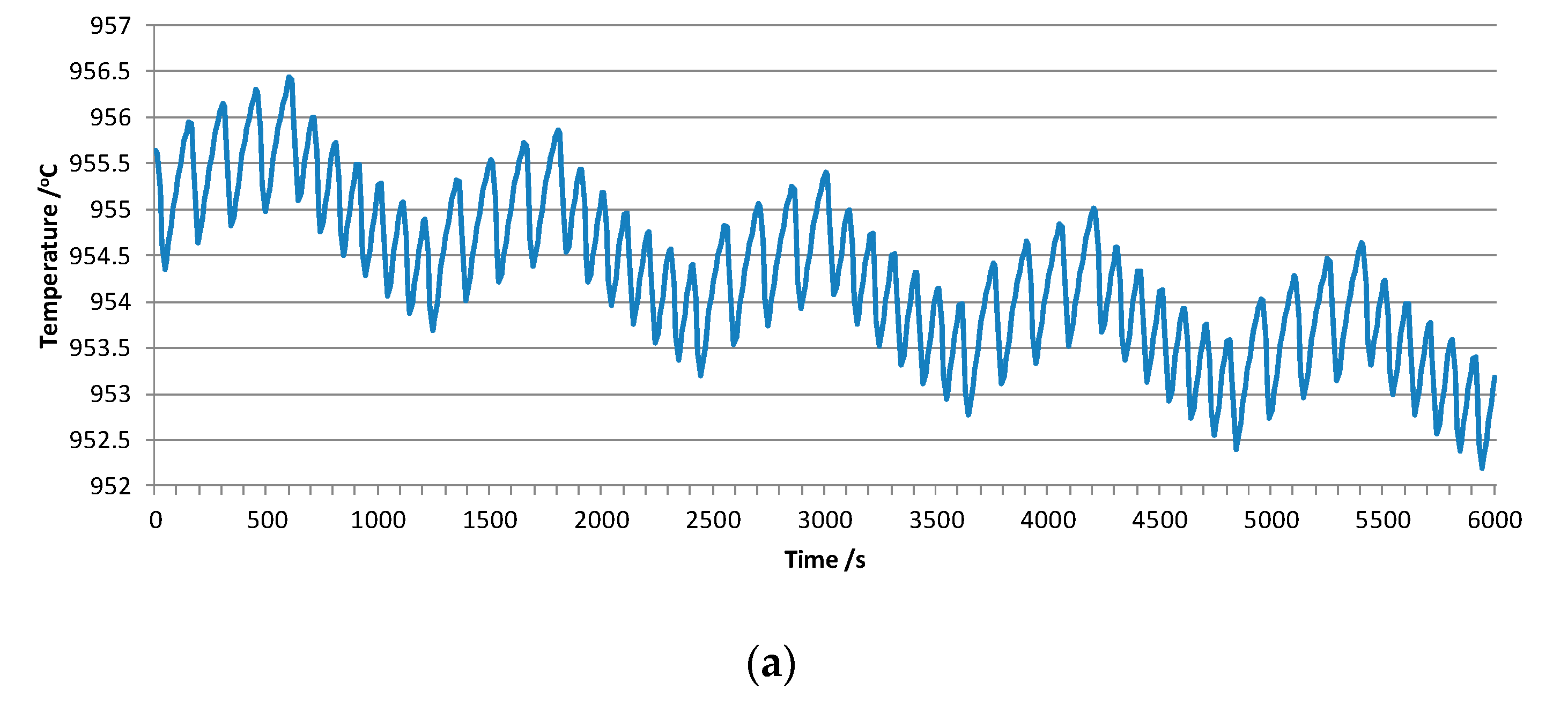
3.1.1. Typical Simulated Curve

Figure 2 shows the temperature fluctuation curve of one cycle in Case 1; the location for temperature measurement is 1 cm from the top surface at the duct end (all the temperatures in context have the same location). The temperature of this point decreases when number 6 feeder works and rises again after feeding. Pulse feeding leads to pulse temperature fluctuation, and said fluctuation is not influenced when number 1, number 3 and number 5 feeders work. The first 600 s is an underfeeding period (feeding interval 150 s) in which the temperature fluctuates up on the whole. The last 600 s is an overfeeding period (feeding interval 100 s) in which temperature fluctuates down on the whole.

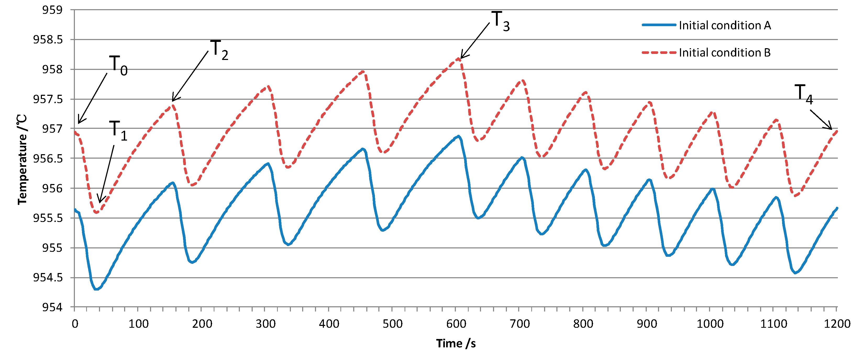
3.1.2. Sensitivity of the Simulated Curve

Five characteristic temperatures were chosen from the simulated curve. As shown in Figure 3, T₀ is the initial temperature; T₁ is the minimum temperature after one feeding shot; T₂ is the temperature after one feeding interval; T₃ is the temperature the after underfeeding period; T₄ is the temperature after one cycle of an underfeeding period and an overfeeding period. T₀ is related to the initial conditions, while the differences between T_i (i = 1,2,3,4) and T₀ determine the shape of the curve. Since this paper focuses on the temperature-change trend, ΔT_i = T_i − T₀ (i = 1,2,3,4) rather than T₀ is focused on in the study.

It is evident that those temperatures are affected by some factors related to the model. According to the model results, the sensitivity of the simulated curve is up to these factors, which are listed in

Table 4. Whether characteristic temperatures are sensitive to several factors.

Characteristic temperature	Element Size ≤ 0.06 m	Initial Condition	Psuck	Thermal Diffusivity of Bath & Metal	Feeding Interval	Differece between Pheat and Pfeeding
T0	NO	Yes	NO	NO	NO	NO
ΔT1	NO	NO	Yes	Yes	NO	NO
ΔT2	NO	NO	Yes	Yes	Yes	Yes
ΔT3	NO	NO	Yes	Yes	Yes	Yes
ΔT4	NO	NO	NO	NO	Little	Yes

(the number is marked when a reasonable change range of the factor leads to a temperature change less than 0.1 °C; a small one is marked for 0.1–0.2 °C; yes is marked for more than 0.2 °C).

As element size changes from 0.05 m to 0.0125 m, above five characteristic temperatures all change less than 0.1 °C, and ΔT_i (i = 1,2,3,4) changes less than 0.01 °C.

Initial conditions include the electrical resistivity and/or thermal conductivity of pot materials, thickness of the cover and so on. Initial conditions may have a great influence on the initial temperature T₀, but little influence on the temperature difference ΔT_i (i = 1,2,3,4), as shown in Figure 3.

Thought P_suck, thermal diffusivity of the bath and metal, and the feeding interval, have considerable influence on ΔT_i (i = 1,2,3 or 2,3), they have little influence on ΔT₄. The only factor that can affect ΔT₄ considerably is “difference between P_heat and P_feeding.”

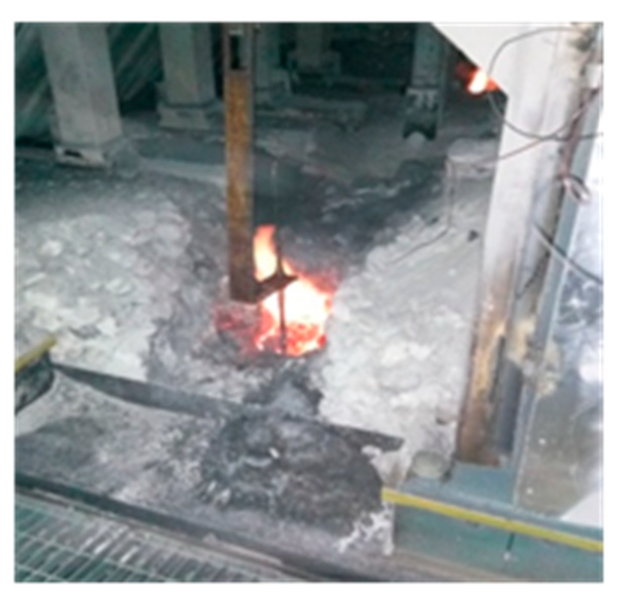
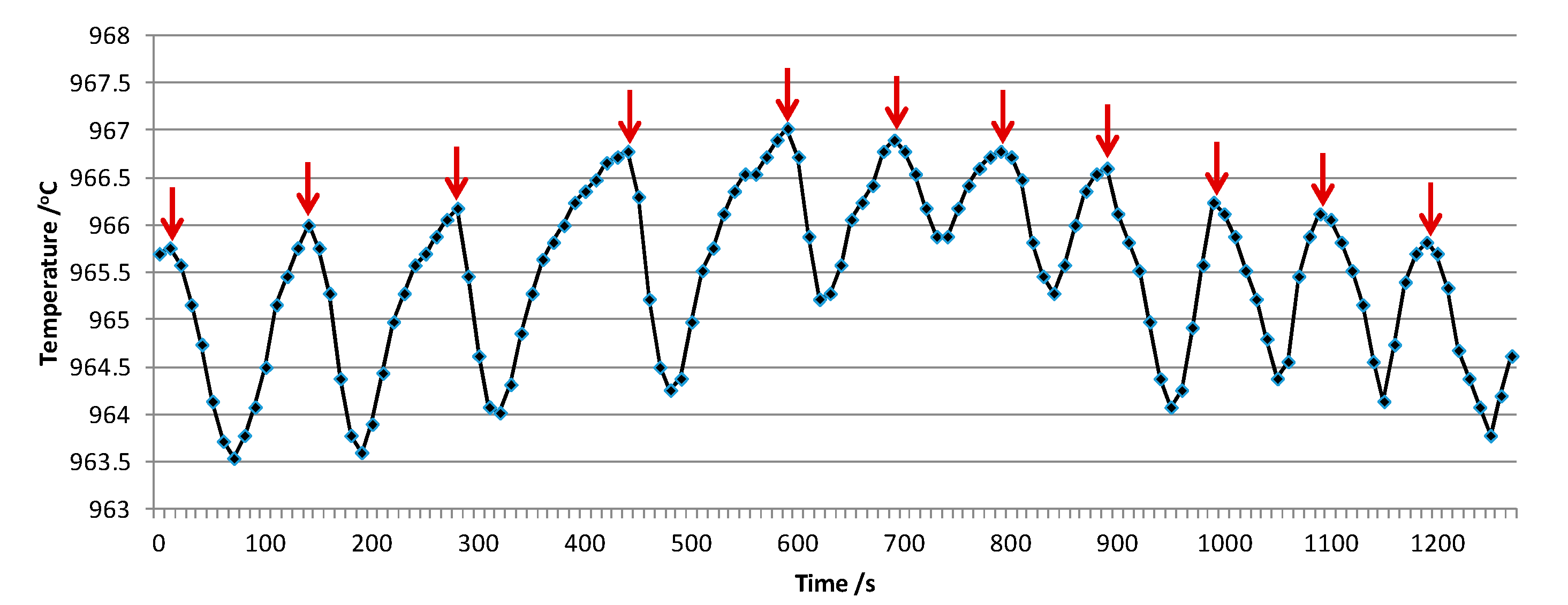
3.1.3. Measurement Data

Experimental conditions:

• Cell amperage: 500 kA.
• Cell conditions: cell voltage was 3.96 v; metal level was 30 cm; bath level was 18 cm.
• Dose weight of six feeders: 1.79–1.82 kg; average 1.8 kg.
• Thermocouple type: K type; precision is 0.1 °C.

Measurement location: 1 cm from the top surface at the duct end. The thermocouple was fixed by a steel support at that location, as shown in Figure 4.

The measurements were made five times repeatedly, and have repeatable results. The standard deviations of ΔT₃ and ΔT₄ in all five measurements are 0.075 and 0.049 °C respectively, which indicates that the uncertainty of temperature change trend in the measurement is less than 0.1 °C.

Figure 5 shows one group of typical temperatures measured on site via the thermocouple, with the same feeding interval system (first four feedings’ interval is 150 s and last six feedings’ interval is 100 s), as shown in Figure 2, which were measured at the same location of the duct end. During temperature measuring, pot condition remained quite good, without other operations influencing it. After a comparison of measurements and simulation results, it can be seen that they have the same fluctuation trend, and the model results basically reflect bath temperature fluctuation in a detailed wave along with the alumina feeding.

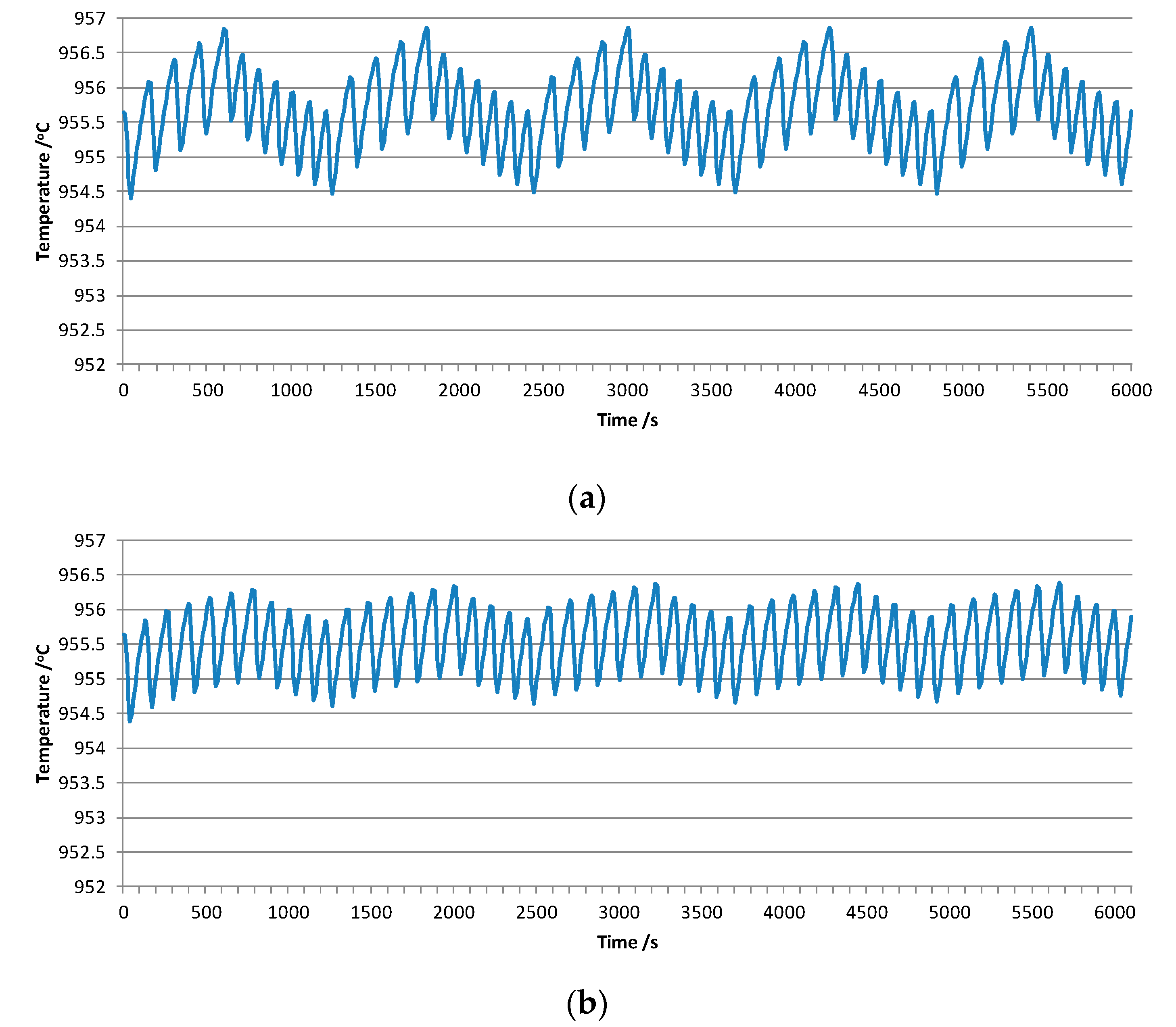
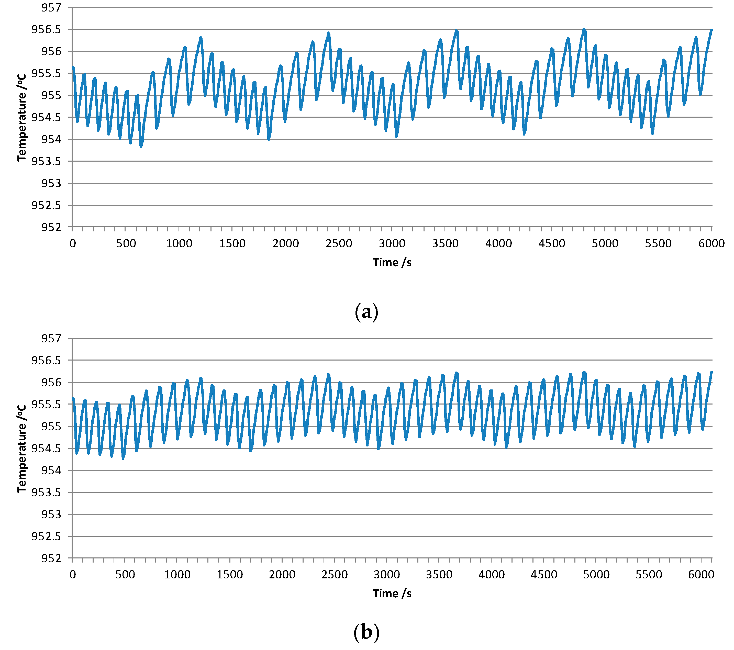
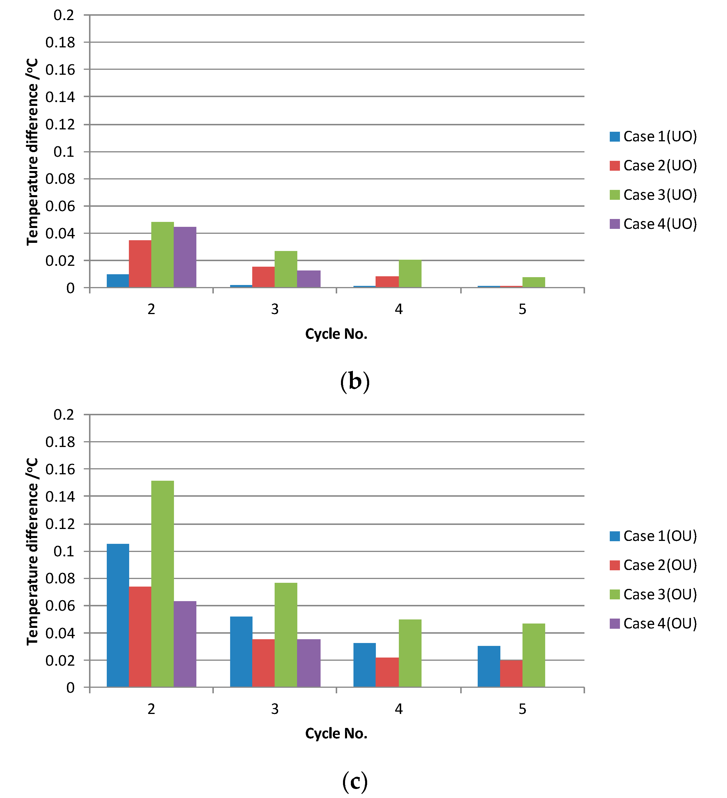
3.2. Influences of Different Feeding Interval Systems

The following definitions are introduced for better discussion: concentration standard feeding interval (flow rate) refers to the feed in a feeding interval (flow rate) when the alumina concentration in the bath remains stable; temperature standard feeding interval (flow rate) refers to the feed in a feeding interval (flow rate) when the bath temperature remains stable.

The above-mentioned “stable” means that the concentration or temperature can periodically return to the initial value within one cycle. The feeding rate (kg/s) is inversely proportional to the feeding interval (s), and that relationship is similar to that between period and frequency.

Figure 6 shows the temperature curves of Cases 1–4 under underfeeding followed by the overfeeding (expressing in UO).

Figure 7 shows the temperature curve results of Cases 1–4 under overfeeding followed by underfeeding (expressing in OU).

In general, temperature fluctuation of Cases 1–4 is within a certain range. The temperature variation between when one cycle ends and another commences can be used to evaluate the temperature change range. The initial state for transient calculations is a stable temperature field. The first cycle is a transition from stable temperature to transient temperature. Therefore, it is only necessary to calculate the difference (ΔT) between ending temperatures and starting temperatures for the last four cycles (only calculating the last two cycles in Case 2); please refer to Figure 8. As shown in Figure 8a, ΔT of cycle number 2 is equal to T₂ − T₁, ΔT of cycle number 3 is equal to T₃ − T₂ and so on.

It can be seen from the Figure 8 that temperature fluctuates less and less as time progress; i.e., temperature becomes more and more stable. The temperature in Case 1 (UO) fluctuates least with ΔT lower than 0.01 °C in each cycle.

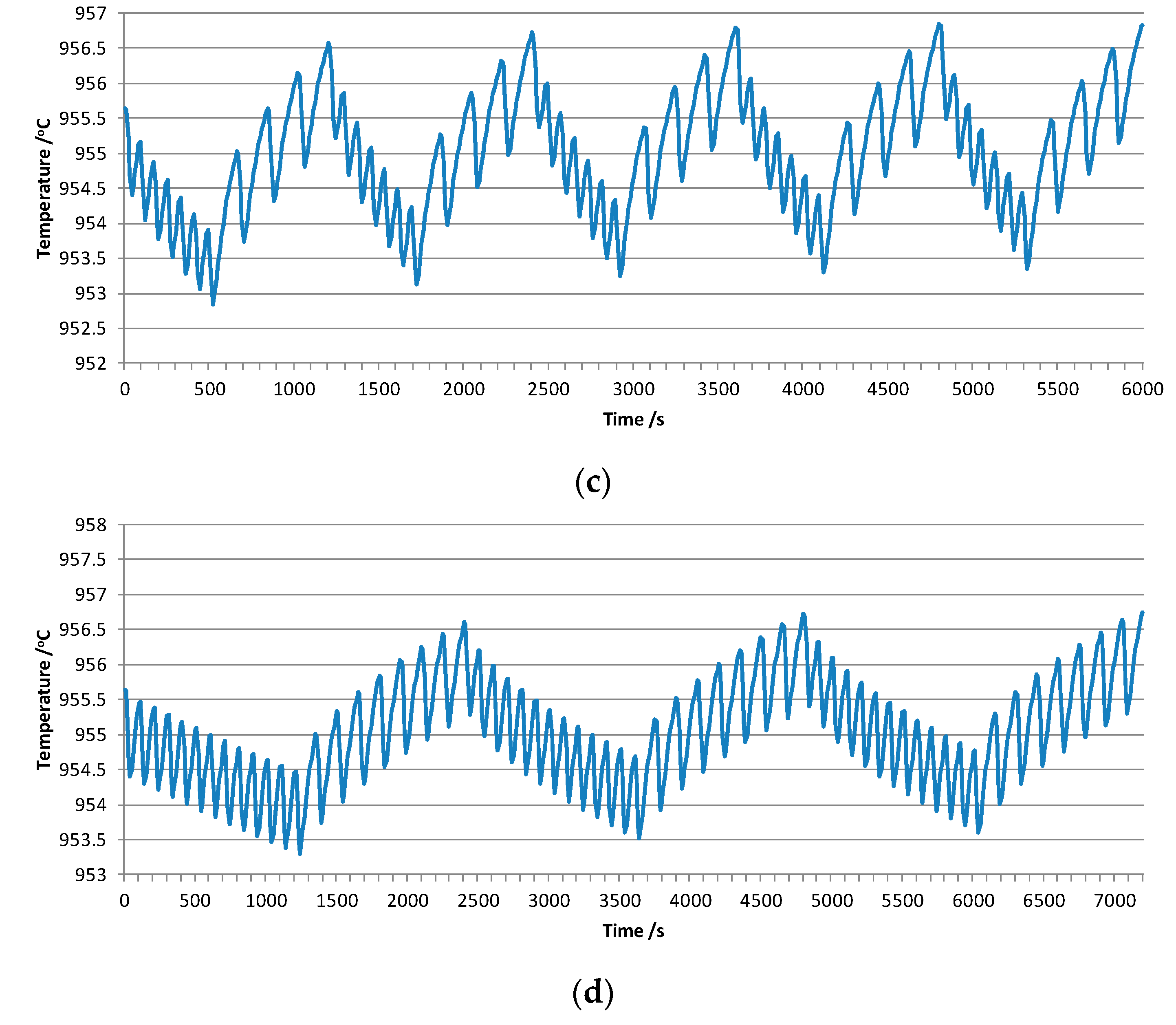
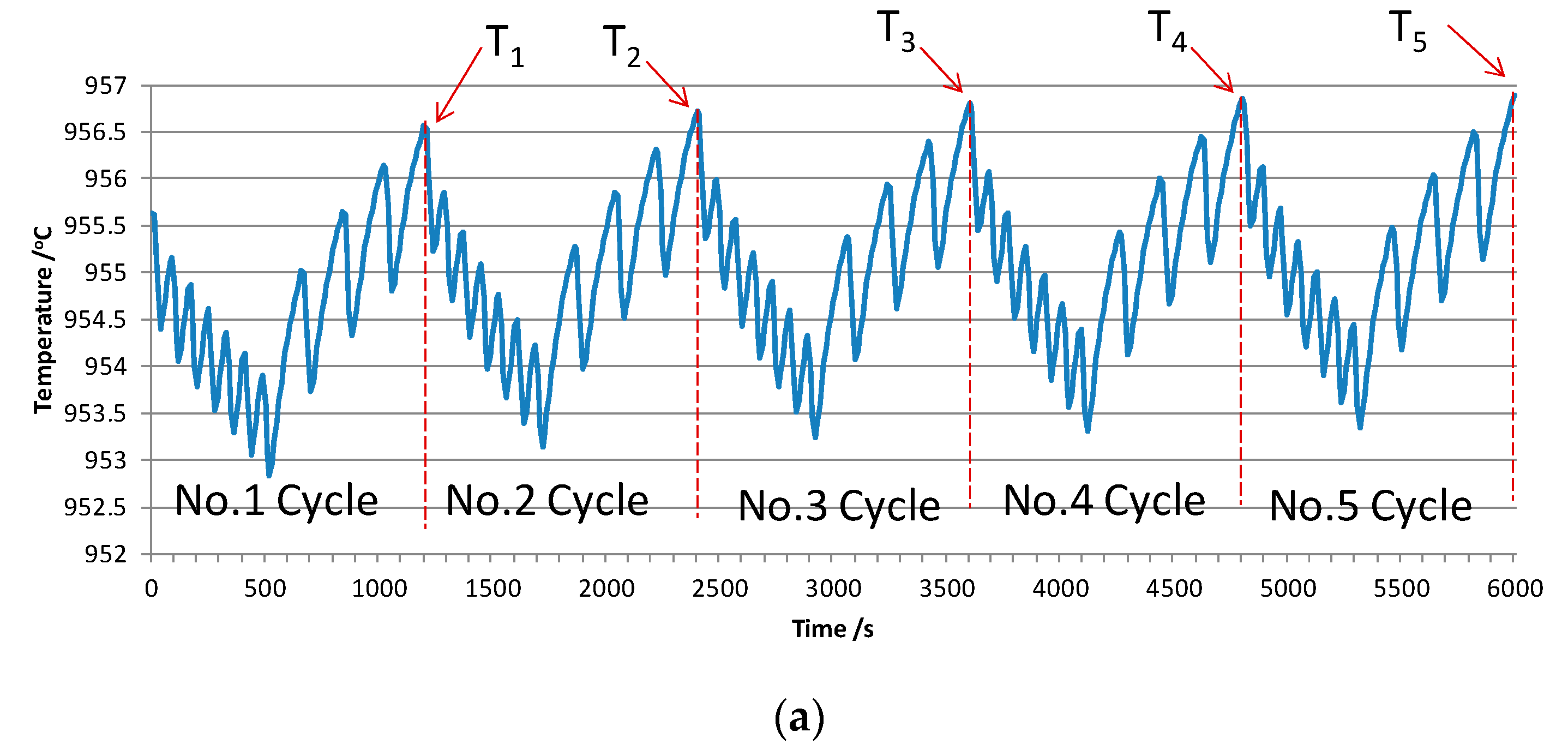
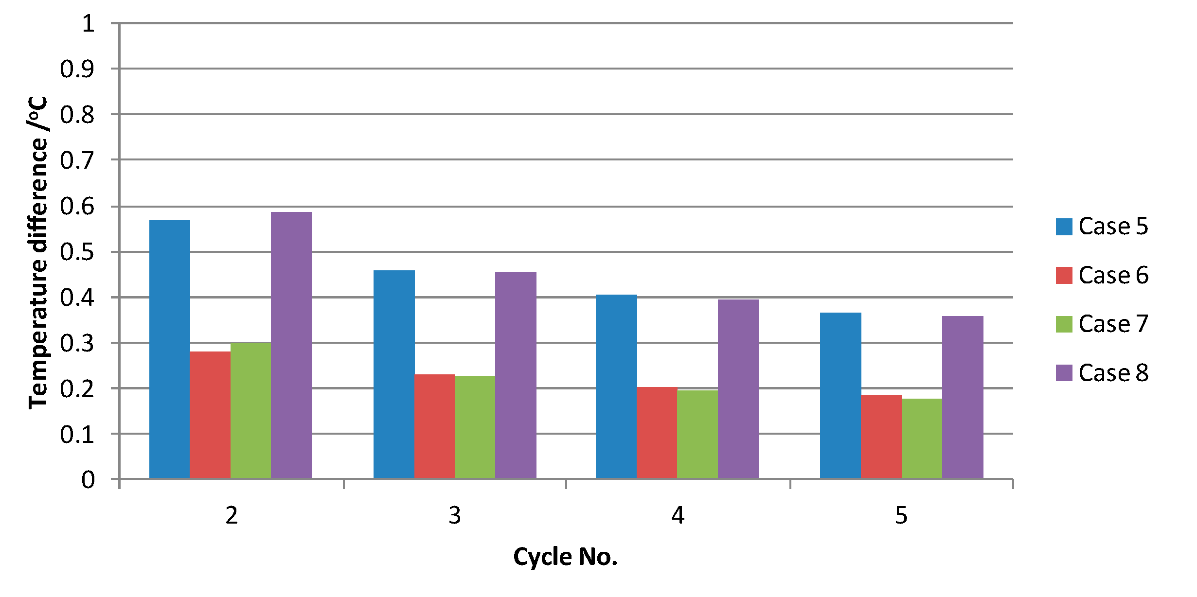
3.3. Influence of the Ratio between P_heat and P_feeding on Temperature Fluctuation

In Cases 5–8, the ratios between P_heat and P_feeding are changed into 0.9, 0.95, 1.05 and 1.1 based on Case 1. Please refer to the temperature fluctuation in Figure 9.

Please refer to ΔT of each cycle for Cases 5–8 in Figure 10.

When P_heat deviates 5% from P_feeding, it means that voltage fluctuates 24 mv in 500 kA pots. Under such circumstances, total ΔT changes 0.9 °C for four cycles, while total ΔT only changes 0.015 °C in Case 1. Whether the P_heat is same as P_feeding is of crucial importance for maintaining bath temperature stability. When P_heat is the same as P_feeding, provided that the feeding interval system is reasonable, there is less influence on the temperature stability, even though through many cycles, the final temperature is still very close to initial temperature.

4. Discussion

The proper feeding interval is of great importance to maintaining the stability of both concentration and temperature, in which the good coordination between underfeeding and overfeeding is the most fundamental factor. If the feeding interval is always longer than the standard interval, alumina concentration will continuously decrease and temperature will sustainably increase no matter how one adjusts the feeding interval. If the feeding interval is always shorter than the standard interval, alumina concentration will continuously increase and temperature will sustainably decrease. The proper feeding interval minimizes underfeeding and overfeeding (such as in Case 1, 20% underfeeding and 20% overfeeding). The durations of underfeeding and overfeeding must be kept within their proper range—not too long. It is better to keep the same extent and duration for underfeeding and overfeeding.

P_heat equal to P_feeding is the prerequisite to maintaining temperature stability. The definition indicates that the average feeding rate when temperature remains stable is the standard feeding rate. On the other hand, if keeping the concentration stable in pots, the average feeding rate shall be equal to the concentration standard feeding rate, which shows that only when the temperature standard feeding rate is kept consistent with the concentration standard feeding rate, can the concentration and temperature both stay stable. Please refer to the analysis as follows:

Concentration standard feeding rate is mainly influenced by potline current and current efficiency and has no close relationship with heat balance, which shows that when potline current and current efficiency are determined, P_feeding is almost determined. The prevailing alumina concentration control program is capable of controlling concentration stability based on the relationship [21] between pot voltage curve slope and alumina concentration. The average feeding rate when alumina concentration stability is under control is nearly equal to the concentration standard feeding rate.

It can be seen from the above simulation results that there will be energy input corresponding to one average feeding rate, to keep temperature stable under such a feeding rate. If the feeding interval is established based on concentration standard feeding rate, temperature fluctuation may become unstable after 3–5 cycles of working, which shows that P_heat is inconsistent with P_feeding and there is a deviation between concentration and temperature standard feeding intervals, and the concentration and temperature cannot return to the initial value together, so it is necessary to correct the gap between P_heat and P_feeding in a timely way by adjusting pot voltage (energy input). If no timely adjustment is conducted, a small ledge solidification and melting process can correct such a deviation when the gap is relatively low, and a great deal of ledge may solidify or melt, eventually resulting in irregular ledge formation when the gap is relatively high.

The uncertainty in the model is due to the simplifications and numerical modeling method. The uncertainty of temperature in the model is less than 0.1 °C. The uncertainty of temperature in the measurements is about 0.1 °C.

Making an assessment of heat balance based on the fluctuation rule of 3–5 cycles can both avoid improper assessment of heat balance due to short-term temperature fluctuations within one cycle, and make a quick assessment without waiting for a longer time. As explained above, making an assessment of heat balance for too long is not good for controlling the heat balance, because the ledge will solidify or melt.

5. Conclusions

Bath temperature is one important indicator with which to assess heat balance. In this paper, a finite element model of a pot transient thermo-electric field is established, considering that the bath will transfer heat to molten aluminum; and the anode, ledge and pot surface will transfer heat to ambient temperature. The simulated temperature curve characteristics are consistent with actual measurements.

It can be seen from the calculation results that each pulse feeding will lead to a short-term pulse fluctuation of pot temperature, and its fluctuation cycle is just the feeding interval. Temperature goes up when underfeeding and it goes down when overfeeding. The alternate conversion between underfeeding and overfeeding is reflected as the cycle of bath temperature fluctuation. The total cycle period equals the total duration of underfeeding and overfeeding. The periodic fluctuation of bath temperature is normal, which does not mean that bath temperature stability is destroyed. Only a development trend of such fluctuations for many cycles can work as the basis for assessing whether the bath temperature is stable or not.

In the paper, the influences on bath temperature fluctuation when P_heat is equal to P_feeding under the different feeding interval systems and when the ratio between P_heat and P_feeding is different under the same feeding interval system are compared and calculated. The feeding interval system has less influence on the temperature fluctuation, and when P_heat deviates 5% from P_feeding, the bath temperature changes about 0.9 °C in the first four cycles, which is a bigger than the fluctuation under different feeding interval systems. Maintaining consistency between P_heat and P_feeding is of crucial importance to maintaining bath temperature stability.

References

1. Bielder, P.; Banta, L. Analysis and Correction of Heat Balance Issues in Aluminum Reduction Cells. In Proceedings of the TMS Light Metals, San Diego, CA, USA, 2–6 March 2003; pp. 441–448. [Google Scholar]
2. Taylor, M.P.; Welch, B.J.; Keniry, J.T. Effect of Electrochemical Changes on the Heat Balance in Aluminum Smelting Cells. J. Electroanal. Chem. Interfacial Electrochem. 1984, 168, 179–192. [Google Scholar] [CrossRef]
3. Liu, J.; Taylor, M.P.; Dorreen, M. Observations of freeze layer formation during heat balance shifts in cryolite-based smelting bath. Int. J. Mater. Res. 2017, 108, 507–514. [Google Scholar] [CrossRef]
4. Valles, A.; Lenis, V.; Rao, M. Prediction of Ledge Profile in Hall-Heroult Cells. In Proceedings of the TMS Light Metals, Las Vegas, NV, USA, 12–16 February 1995; pp. 309–313. [Google Scholar]
5. Ahmed, H. Prediction of the Thermal Aspects of Egyptalum Prototype High-amperage Pre-baked Aluminum Reduction Cells. In Proceedings of the TMS Light Metals, San Francisco, CA, USA, 27 February–3 March 1994; pp. 333–338. [Google Scholar]
6. Taylor, M.P.; Liu, X.; Fraser, K.J. The Dynamics and Performance of Reduction Cell Electrolytes. In Proceedings of the TMS Light Metals, Anaheim, CA, USA, 18–22 February 1990; pp. 259–266. [Google Scholar]
7. Pei-lin, D.; Heng, W.; Jun, H. Effect of feeding in aluminum reduction cell on electrolyte temperature. Chin. J. Nonferrous Met. 2016, 26, 430–438. [Google Scholar]
8. Thonstad, J.; Solherim, A.; Rolseth, S. The dissolution of alumina in cryolite melts. In Essential Readings in Light Metals; Bearne, G., Ed.; Springer: Cham, Switzerland, 2016. [Google Scholar]
9. Thomas, H. Numerical Simulation and Optimization of the Alumina Distribution in an Aluminium Electrolysis pot. Ph.D. Thesis, École Polytechnique Fédérale de Lausanne, Lausanne, Switzerland, 2011. [Google Scholar]
10. Li, M.; Gao, Y.; Bai, X.; Li, Y.; Hou, W.; Wang, Y. Simulation of alumina particle dissolution in 300 kA aluminum electrolytic cell. Chin. J. Nonferrous Metals 2017, 27, 1738–1747. [Google Scholar]
11. You-Cai, L. Kinetics Study of Alumina Crust Formation and Dissolution in Aluminum Electrolysis. Ph.D. Thesis, North East University, Shenyang, China, 2018. [Google Scholar]
12. Kobbeltvedt, O.; Moxnes, B.P. On the Bath Flow, Alumina Distribution and Anode Gas Release in Aluminium Cells. In Proceedings of the TMS Light Metals, Orlando, FA, USA, 9–13 February 1997; pp. 257–264. [Google Scholar]
13. Lavoie, P.; Taylor, M.P.; Metson, J.B. A review of alumina feeding and dissolution factors in aluminum reduction cells. Metall. Mater. Trans. B 2016, 47, 2690–2696. [Google Scholar] [CrossRef]
14. McFadden, F.J.; Welch, B.J.; Whitfield, D. Control of Temperature in Aluminium Reduction Cells—Challenges in Measurements and Variability. In Proceedings of the TMS Light Metals, New Orleans, LA, USA, 11–15 February 2001; pp. 1171–1178. [Google Scholar]
15. Soares, F.; Oliveira, R.; Castro, M. Bath Temperature Inference through Soft Sensors Using Neural Networks. In Proceedings of the TMS Light Metals, Washington, DC, USA, 14–18 February 2010; pp. 467–472. [Google Scholar]
16. Bruggeman, J.N.; Danka, D.J. Two-dimensional Thermal Modeling of the Hall- Héroult Cell. In Proceedings of the TMS Light Metals, Anaheim, CA, USA, 18–22 February 1990; pp. 203–209. [Google Scholar]
17. Berge, B.; Grjotheim, K.; Krohn, C.; Næumann, R.; Tørklep, K. Recent studies of convection in commercial aluminum reduction cells. Metall. Trans. 1973, 4, 1945–1952. [Google Scholar] [CrossRef]
18. Grjotheim, K.; Krohn, C.; Naeumann, R.; Tørklep, K. On convection in aluminum reduction cells. Metall. Trans. 1970, 1, 3133–3141. [Google Scholar]
19. Fuqiang, W.; Qinsong, Z.; Wei, L.; Youjian, Y.; Zhaowen, W. Impact of local cathode electrical cut-off on bath-metal two-phase flow in an aluminum reduction cell. Metals 2020, 10, 110. [Google Scholar]
20. Zhibin, Z.; Yuqing, F.; Philip, S.M.; Peter, J.W.; Zhaowen, W.; Mark, C. Numerical modeling of flow dynamics in the aluminum smelting process: Comparison between air–water and co2–cryolite systems. Metall. Mater. Trans. B 2017, 48, 1200–1216. [Google Scholar]
21. Liu, Y.; Jie, L. Modern Aluminum Electrolysis; Metallurgy industry Press: Beijing, China, 2008. [Google Scholar]
22. Kuschel, G.I.; Welch, B.J. Further Studies of Alumina Dissolution under Conditions Similar to Cell Operation. In Proceedings of the TMS Light Metals, New Orleans, LA, USA, 17–21 February 1991; pp. 112–118. [Google Scholar]
23. Peter, K. Theory; ANSYS, Inc.: Canonsburg, PA, USA, 2005. [Google Scholar]
24. Fletcher, C.A.J. Galerkin Finite-Element Methods. In Computational Galerkin Methods; Springer Series in Computational Physics; Springer: Berlin/Heidelberg, Germany, 1984. [Google Scholar]
25. Ansys, Handbook Ansys 9; Ansys, Inc.: Canonsburg, PA, USA, 2005.
Figure 1. 3D thermo-electric field quarter model built by ANSYS.
Metals 10 00379 g001
Figure 2. Temperature fluctuation curve of one cycle in case 1 (arrow refers to feeding moment of number 6 feeder).
Metals 10 00379 g002
Figure 3. Sensitivity of the simulated curve.
Metals 10 00379 g003
Figure 4. Thermocouple location.
Metals 10 00379 g004
Figure 5. Temperatures measured on site via thermocouple (arrow refers to feeding moment of number 6 feeder).
Metals 10 00379 g005
Figure 6. Temperature curves of Cases 1–4 under underfeeding followed by overfeeding. (a) Case 1 (UO), underfed (t = 150 s)–overfed (t = 100 s); (b) Case 2 (UO), underfed (t = 130 s)–overfed (t = 110 s); (c) Case 3 (UO), underfed (t = 180 s)–overfed (t = 80 s); (d) Case 4 (UO), underfed (t = 150 s)–overfed (t = 100 s).
Metals 10 00379 g006aMetals 10 00379 g006b
Figure 7. Temperature curves of Cases 1-4 under overfeeding followed by underfeeding. (a) Case 1 (OU), overfed (t = 100 s)–underfed (t=150 s); (b) Case 2 (OU), overfed (t = 110 s)–underfed (t=130 s); (c) Case 3 (OU), overfed (t = 80 s)–underfed (t = 180 s); (d) Case 4 (OU), overfed (t = 100 s)–underfed (t = 150 s).
Metals 10 00379 g007aMetals 10 00379 g007b
Figure 8. ΔT of each cycle. (a) Illustration of ΔT; (b) underfeeding followed by overfeeding; (c) overfeeding followed by underfeeding.
Metals 10 00379 g008aMetals 10 00379 g008b
Figure 9. Temperature fluctuation curve under different ratios between Pheat and Pfeeding. (a) Case 5 (Pheat/Pfeeding = 0.9); (b) Case 6 (Pheat/Pfeeding = 0.95); (c) Case 7 (Pheat/Pfeeding = 1.05); (d) Case 8 (Pheat/Pfeeding = 1.1).
Metals 10 00379 g009aMetals 10 00379 g009b
Figure 10. ΔT of each cycle for Cases 5–8 under different ratios of Pheat to Pfeeding.
Metals 10 00379 g010