Abstract
As-quenched low-carbon martensitic steels (<0.2 wt.% C) contain auto-tempered carbides. Auto-tempering improves the work hardening and upper-shelf impact energy; however, an efficient characterization method to determine the degree of auto-tempering has not been available. This paper demonstrates an efficient image processing tool that calculates the relative auto-tempered carbide fraction by analyzing scanning electron microscope micrographs. By the process of image segmentation, the qualitative volume fraction of auto-tempered carbides can be determined, and an associated color map produced, which distinguished the levels of auto-tempering. This image processing tool could become useful for the optimization of new low-carbon steel’s mechanical properties.
1. Introduction
High strength, excellent toughness, and good weldability are three steel properties that are highly desirable for mechanical applications [1]. Low-carbon (<0.2%) high-strength steels possess these three properties and, thus, are commonly used in structural applications [2]. For example, in the automobile industry, low-carbon high-strength structural steels offer the possibility of weight reduction while maintaining or increasing component strength [3]. The microstructure of martensite is a major contributor to the attainment of these desirable properties [4]. Martensite is formed by a diffusionless shear mechanism when austenite is cooled rapidly to room temperature [5]. In the case of low-alloy steels, this rapid cooling normally requires water quenching. The morphology of martensite in low-carbon low-alloy steels are lath like [5,6]. The diffusionless shear mechanism produces martensite that is supersaturated with carbon when compared with the equilibrium ferritic state of the steel. However, when low-carbon steels with high martensitic start temperatures (Ms) are quenched, in addition to martensite, fine carbides can form [7]. This phenomenon is called auto-tempering [5,7,8] and it has been shown to improve the work-hardenability of high-strength steels [9] and the upper-shelf impact energy [10].
Due to the small sizes of the carbides formed during auto-tempering, electron microscopy is the most optimal characterization technique to investigate the carbides [2]. By analyzing electron micrographs, it is possible to differentiate between regions of high and low auto-tempering. To the authors’ knowledge, no method has been produced to quantitatively analyze the degree of auto-tempering in an efficient manner. Due to the very small fractions of auto-tempered carbides accompanying martensite formation, dilatometers, which depend on volumetric changes, are not sensitive enough to reveal their formation.
Image processing tools have been widely used in metallography as they are fast at analyzing specific features, qualitatively and quantitatively, from a micrograph when compared to a human being. Mesquita et al. [11] used image analysis to evaluate and compare carbide coarsening by binarizing secondary electron grey images. Komenda [12] utilized the Image Classifier software package integrated with MicroGOP2000/s system to quantitatively analyze the phases in sintered steels and the γ’ particle size distribution in nickel-based superalloys. Albuquerque et al. [13] developed an automated image processing tool based on artificial neural networks for quick analysis of multiple micrographs obtained from cast iron.
This paper demonstrates an image processing methodology to qualitatively analyze the auto-tempered carbides formed in as-quenched low-carbon steels. Electron micrographs were analyzed using bespoke software that was developed using the MATLAB (version 2018b, MathWorks, Inc., Natick, MA, USA) image processing toolbox.
2. Materials and Methods
A 12 mm thick hot-rolled low-carbon steel plate was supplied by SSAB Europe Oy with the composition shown in Table 1. A glow discharge optical emission spectroscopy (GDOES) (Spectruma GDA 750 Analyser, Spectruma Analytik GmbH, Hof, Germany) was used to determine the bulk composition. Cylindrical specimens, 6 mm in diameter and 9 mm in length, were machined from the plates with their long axes parallel to the rolling direction. Austenitization and quenching of the steel was achieved by using a Gleeble 3800 thermomechanical simulator (Dynamic Systems Inc., Poestenkill, NY, USA). The cylinders were heated at a rate of 10 °C/s to 950 °C and held for 2 min to ensure austenitization, and then cooled by water cooled aluminum jaw-carriers at a rate of 100 °C/s.

Table 1.
The mean chemical composition (Spectruma GDA 750 Analyzer) of the studied steel [2,8].
Cross-sections from the heat-treated cylindrical specimens were cut transverse to the long axes of the cylinders at the position of the control thermocouple. It was found previously [2] that hot mounting auto-tempered martensitic steel samples induces additional tempering. To prevent this, the samples were cold mounted with an epoxy resin (Struers EpoFix Resin, Struers ApS, Ballerup, Denmark) mixed with a hardener (Struers EpoFix, Struers ApS, Ballerup, Denmark), cured and left to harden for 24 h. The mounted samples were polished to a mirror finish using 0.04 µm colloidal silica, and subsequently etched with a 2% Nital solution. The microstructures were examined with a field emission scanning electron microscope (FE-SEM) (Zeiss Sigma, Carl Zeiss AG, Oberkochen, Germany) using a 5 kV acceleration voltage and an InLens secondary electron detector.
A custom program that utilizes the Image Processing Toolbox in MATLAB (version 2018b, MathWorks, Inc., Natick, MA, USA) was designed and used to study the precipitates that forms as a result of auto-tempering. The methodology used to make the quantification is as follows:
- (a)
- A SEM micrograph from the region of interest containing precipitates is selected, e.g., as shown in Figure 1a.
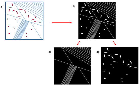 Figure 1. Schematic images showing the routine used to isolate the precipitates in field emission scanning electron microscopy (FE-SEM) images of auto-tempered martensite.
 - (b)
- Binarization technique is used to convert the image into black and white pixels, as shown in Figure 1b.
- (c)
- The grain and lath boundaries are larger than the carbide precipitates. These features can be removed from the image by applying an appropriate threshold number of pixels, so that features which represent low-angle or high-angle grain boundaries are discriminated and removed from the image, as shown in Figure 1c. The resultant image comprising of groups of pixels that are smaller than the threshold value shows the precipitates, Figure 1d. While the lath and grain boundaries were long thin features, the precipitates were small and roughly elliptical. Distinguishing the precipitates from the other features was based on a two-staged approach. In the first stage, large features were perished, which removes majority of the grain and lath boundaries. The remaining features were mainly the precipitates and some portions of the grain boundaries that were not extracted as coherent features due to the limitations of the image resolution. Therefore, in the second stage, the ratios of the lengths of the major and minor axes of the features were calculated and all the features with a ratio larger than a specified threshold (30 pixels) were deleted as lath or grain boundaries.
- (d)
- The image of the precipitates were further processed by dividing it into a matrix of equi-sized boxes (100 by 100 boxes). The ratio of white pixels to the total number of pixels in each box was calculated, and depending on the ratio, the region was designated a particular color indicating the local area fraction of auto-tempered carbides, as shown in Figure 2. The highly auto-tempered regions (yellow) were designated as those in which the apparent area fraction of the auto-tempered carbides within a given box exceeded 10%. The regions showing a low local area fraction of auto-tempered carbides were those in which box area fractions were in the range 1–10% (green). Boxes showing area fractions less than 1% were designated non-auto-tempered (blue).
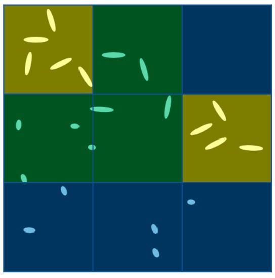 Figure 2. Schematic diagram of a precipitate image divided into square boxes and colored according to the degree of auto-tempering. The apparent local area fraction of auto-tempered carbides decreases from yellow through green to blue.
An alternative method that could be used to benchmark the image analysis techniques could be by visually inspecting the micrographs. However, this method cannot be standardized and will be subjected to human errors. Therefore, visual inspection cannot be used to ‘benchmark’ the image analysis technique.
3. Results and Discussion
The quenched steel had a typical lath martensite microstructure with carbide precipitates resulting from auto-tempering, as shown in Figure 3. The microstructure consisted of (1) coarse martensite laths with a high-volume fraction of carbides relative to the other features in the microstructure, (2) thin martensite laths without carbides, and (3) dark islands with minimal or no carbides [8]. These results were consistent with the observations made by Morsdorf et al. [4]. The martensite start temperature, Ms, of this steel was previously determined as 435 °C [14]. Due to the high Ms temperature, the formation of martensite was followed by the precipitation of carbides. The precipitates have been previously identified as cementite [2]. This observation is also consistent with the observations of Speich [15], where only cementite precipitates form in quenched martensite with a carbon content <0.2 wt.%. As stated by Morsdorf et al. [4], in the case of relatively high Ms temperatures, the formation of coarse laths was favored just below the Ms temperature where the austenite was soft and had a low defect density thereby providing relatively low resistance to the growth of martensitic laths. Upon further cooling, the resistance produced by the retained austenite progressively increases by the increase in the density of dislocations needed to plastically accommodate the previously formed martensite laths and the decreasing temperature. This phenomenon causes auto-catalytic triggering of the thin lath formation at lower temperatures. Untempered martensitic regions were the last to form at temperatures close to the martensite finish temperature, Mf. Due to the effect of temperature on the kinetics of precipitate nucleation and growth, the volume fraction of carbides that can form in any given lath can be expected to decrease as the temperature at which the lath forms decrease.
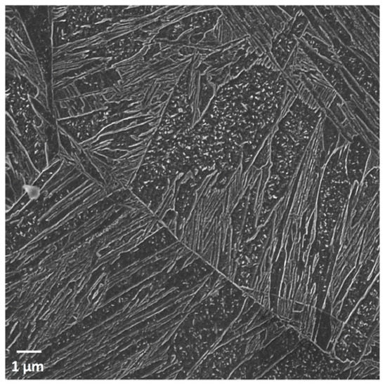
Figure 3.
SEM secondary electron micrograph of a quenched sample.
The micrograph in Figure 3 was grayscaled, where the pixels at grain boundaries and precipitates have high intensities while the pixels in the martensite matrix have lower intensities. Binarization of the SEM image was performed by applying a threshold to the intensity values to ensure that the non-matrix features were positive while the background was zero, as shown in Figure 4a. Further, the larger features, such as grain and lath boundaries (Figure 4b), were separated from the smaller sized precipitates (Figure 4c), as described in Section 2.
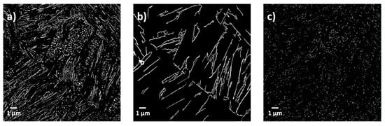
Figure 4.
(a) Binary image of SEM micrograph in Figure 3. (b,c) were segmented from (a) using an appropriate threshold value of 30 pixels. (b) Binary image of the grain boundaries (pixels ≥ 30). (c) Binary image with only the precipitates (pixels < 30).
By using the custom MATLAB® program (see Appendix A), the calculated phase fraction of auto-tempered precipitates from Figure 4c was 3.02%. However, this is an overestimation as Thermo-Calc [16] software predicted the equilibrium volume fraction of cementite at 23 °C as 1.84%.
There is no measurement error per image as that is limited to the resolution of the selected SEM micrograph and the pixels as computed by MATLAB. Depending on what information is required, the qualitative volume fraction can be either obtained from one image, or multiple images, if the average volume fraction over a larger area should be considered. As the distribution of auto-tempered carbides is constant throughout our specimens, information from three images each being discretized into 10,000 boxes was sufficient to get a good overall estimation.
The combined effect of two factors explain the overestimation: (1) Some rod-shaped cementite particles can be smaller than the pixel size used and (2) cementite precipitates are embedded within the martensitic matrix irregularly, which leads to them sticking out from the etched surface at various angles, as shown in Figure 5. This makes the dimension relevant for calculating the area (and volume) fraction i.e., as seen in Figure 5, “dc” appears as the larger size “da”. The finite size of the electron beam produces a secondary electron (SE) signal outside the center-point of the beam, which increases the apparent size of small objects, ultimately defining the resolution limit of the microscope. Non-metallic inclusions were not a problem in our sample due to the cleanness of the steel.
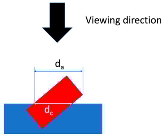
Figure 5.
Schematic cross-section through a polished and etched surface showing the carbide dimension that would lead to a correct estimate of the carbide volume fraction (dc) and the corresponding apparent dimension (da) seen projected onto the plane of the scanned secondary electron (SE) image.
Despite these drawbacks, even the apparent carbide volume fraction can provide useful qualitative information about the local area fraction of auto-tempered carbides.
The local area fractions of auto-tempered carbides were best visualized using a color map, as shown in Figure 6. Figure 7 shows a histogram of the frequencies of the different local area fractions of auto-tempered carbides.
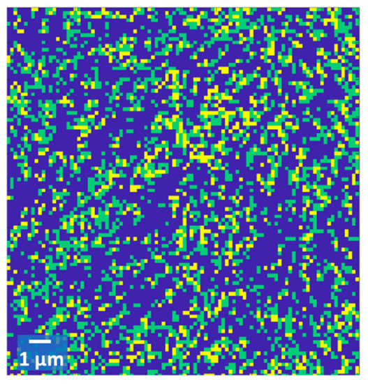
Figure 6.
Color map representing the local area fraction of auto-tempered carbides in the sample. Apparent area fractions of auto-tempered carbides; >10% yellow, 1–10% green, and <1% blue.
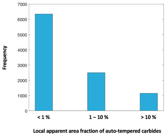
Figure 7.
Histogram showing the distribution of local area fractions of auto-tempered carbides.
To demonstrate how the image processing tool can be utilized in practice, a steel sample with the same chemical composition as that above was austenized and water-quenched at 1000 °C/s in a similar way to that described in [2]. The SEM micrograph of the resulting microstructure is shown in Figure 8a. It is clear that the carbides were not as abundant as they were in the micrograph, as shown in Figure 3, which was from a specimen quenched at 100 °C/s. By using the image segmentation technique to isolate the precipitates from the matrix, the apparent volume fraction of the carbides resulting from auto-tempering was found to be 2.74%, i.e., a reduction of 0.28% area fraction compared to that found in the samples cooled at 100 °C/s. The color map showing the apparent local carbide area fractions can be seen in Figure 8b. Qualitative comparisons of the relative local apparent area fraction of auto-tempered carbides can be conducted by comparing the histograms of carbide area fraction distributions from both specimens, as shown in Figure 9 (brown for the specimen cooled at 1000 °C/s and blue for the specimen cooled at 100 °C/s). The histograms were constructed from data gathered from three images totaling to 30,000 indexed boxes. The bars representing those boxes with <1% apparent area fraction of precipitates were almost the same for both the cooling rates. The histograms show that cooling at 100 °C/s produces a higher incidence of boxes with apparent carbide fractions >10% while cooling at 1000 °C/s increases the incidence of boxes with apparent carbide fractions 1–10%. This is as would be expected since the lower the cooling rate the greater the time available for carbide precipitation in the laths formed close to Ms resulting in denser and larger carbide formation. Since the precipitates which form during cooling at the high rate are smaller than those forming during slower cooling, the proportion of the microstructure showing local apparent carbide fractions in the range 1–10% is higher.
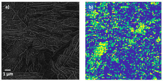
Figure 8.
(a) SEM images of the Gleeble austenitized and subsequently water-quenched steel sample (1000 C/s). (b) Though the use of the custom MATLAB computer program, a color map that indicates the local area fraction of auto-tempered carbides within the highly auto-tempered regions. Apparent area fractions of auto-tempered carbides; >10% yellow, 1–10% green, and <1% blue.
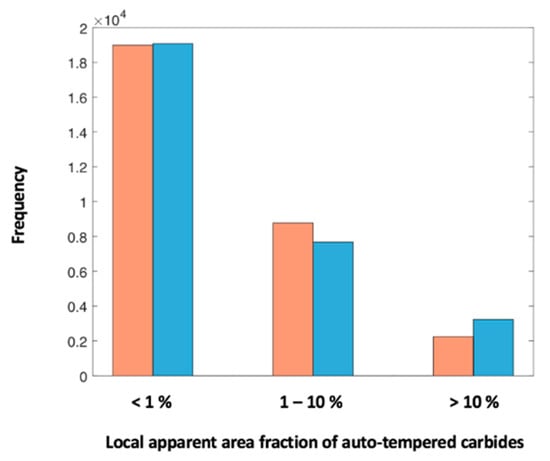
Figure 9.
Histogram where the degree of auto-tempering in the specimens cooled at 100 °C/s is represented by the blue bars and the specimens cooled at 1000 °C/s by the brown bars.
This study has shown that the custom image processing program was able to qualitatively estimate and compare the volume fractions of the auto-tempered carbides formed in as-quenched low carbon steels.
4. Conclusions
A custom-built image processing program using MATLAB has been used to estimate the fraction of auto-tempered carbides in an as-quenched low-carbon martensitic steel. The program binarized SEM micrographs to intensify only the boundaries and precipitates keeping the background at zero intensity. The grain and lath boundaries were removed from the binarized image by applying an appropriate threshold number of pixels. The resultant image comprises of groups of pixels smaller than the threshold value indicating the precipitates. This image gives the qualitative area fraction of the precipitates. This could further be processed into a color map indicating the apparent local area fractions of the auto-tempered carbides, where the high, low and non-auto-tempered regions were designated with yellow, green, and blue, respectively. The use of the image processing program was then demonstrated using as-quenched low-carbon steel samples cooled at 100 °C/s and 1000 °C/s.
Author Contributions
Conceptualization, S.R.B. and D.P.; methodology, S.R.B. and D.P.; software, S.R.B.; validation, S.R.B. and T.H.; formal analysis, S.R.B. and D.P.; investigation, S.R.B. and D.P.; resources, S.R.B. and D.P.; data curation, S.R.B; writing—original draft preparation, S.R.B; writing—review and editing, S.R.B., D.P., A.J. and T.P.D.; visualization, S.R.B.; supervision, D.P.; project administration, J.K.; funding acquisition, D.P. and J.K. All authors have read and agreed to the published version of the manuscript.
Funding
The authors are grateful for financial support from the European Commission under grant number 675715-MIMESIS-H2020-MSCA-ITN-2015, which is a part of the Marie Sklodowska-Curie Innovative Training Networks European Industrial Doctorate Programme. T.P. Davis is funded by the Clarendon Scholarship from the University of Oxford and United Kingdom’s Engineering and Physical Sciences Research Council Fusion Centre for Doctorial Training [EP/L01663X/1].
Acknowledgments
The authors would also like to thank Pasi Suikkanen from SSAB Europe Oy for his support. The support of SSAB Europe Oy in providing the steel studied is acknowledged.
Conflicts of Interest
The authors declare no conflict of interest. The funders had no role in the design of the study; in the collection, analyses, or interpretation of data; in the writing of the manuscript, or in the decision to publish the results.
Appendix A
Image processing code for auto-tempering quantification:
cut=110; %sets a threshold level. All pixels below that intensity value will be colored black, the others white
% use imtool to determine the best threshold value
areasize = 350; %maximum area of objects that should be kept
ratiothreshold = 4;
I = imread(‘‘); % Read image here
I = rgb2gray(I);
%I = imsharpen(imresize(I,[2000 3000]),’Radius’,2,’Amount’,1);
% threshold the image to turn into logical image
I(I<cut) = 0;
I(I>=cut) = 255;
%Remove all small objects (meaning substact all the Martensite fraction)
BW2 = bwareaopen(I,areasize);
% Subtract the Image without Martensite (BW2) from the original BW image
% (I) to get image with Martensite only
BW = imbinarize(I)-BW2;
BWstat = BW;
%imshow(BW);
%Extract informations about remaining featues
areastatistics = regionprops(logical(BW),’MajorAxisLength’,’MinorAxisLength’,’PixelList’);
%create an empty image where the features to delete will be writen in
BWloss = uint8(zeros(1034,1037));
%search for features with an aspect ratio larger than the threshold and
%mark them
for i = 1:length(areastatistics)
if(areastatistics(i).MajorAxisLength/areastatistics(i).MinorAxisLength>ratiothreshold)
k = (areastatistics(i).PixelList);
[klen,~] = size(k);
for kcount = 1:klen
BWloss(k(kcount,2),k(kcount,1)) = 1;
end
end
end
BWnew = imbinarize(BW)-imbinarize(BWloss);
BW3 = bwareaopen(BWnew, 30);
R = BWnew-BW3;
BW2 = imcrop(BW2,[0 0 1000 1000]); % Grain and Lath boundaries
R = imcrop(R,[0 0 1000 1000]); % Only precipitates in image
ca = mat2cell(R,10*ones(1,size(R,1)/10),10*ones(1,size(R,2)/10));
for i = 1:100
for j = 1:100
numWhitePixels(i,j) = sum(sum(ca{i,j}));
end
end
numWP = sum(sum(numWhitePixels));
matRatio = (numWhitePixels/100)*100;
y = matRatio;
%Generate Colour map
y(y < 1) = 0;
y(y >= 10) = 100;
y(y > 1 & y < 10) = 40;
%Generate Colour map
image(y)
References
- Béranger, G.; Henry, G.; Sanz, G. The Book of Steel; Intercept Ltd.: Andover, UK, 1996. [Google Scholar]
- Babu, S.R.; Jaskari, M.; Järvenpää, A.; Porter, D. The effect of hot-mounting on the microstructure of an As-Quenched auto-tempered low-carbon martensitic steel. Metals 2019, 9, 550. [Google Scholar] [CrossRef]
- Hutchinson, B.; Hagström, J.; Karlsson, O.; Lindell, D.; Tornberg, M.; Lindberg, F.; Thuvander, M. Microstructures and hardness of as-quenched martensites (0.1–0.5%C). Acta Mater. 2011, 59, 5845–5858. [Google Scholar] [CrossRef]
- Morsdorf, L.; Tasan, C.C.; Ponge, D.; Raabe, D. Acta Materialia 3D structural and atomic-scale analysis of lath martensite: Effect of the transformation sequence. Acta Mater. 2015, 95, 366–377. [Google Scholar] [CrossRef]
- Bhadeshia, H.K.D.H.; Honeycombe, R.W.K. Steels: Microstructure and Properties, 4th ed.; Butterworth-Heinemann: Oxford, UK, 2017. [Google Scholar]
- Krauss, G. Steels: Heat Treatment and Proceesing Principles; ASM International: Cleveland, OH, USA, 1990. [Google Scholar]
- Krauss, G. Martensite in steel: Strength and structure. Mater. Sci. Eng. A 2002, 273–275, 40–57. [Google Scholar] [CrossRef]
- Ramesh Babu, S.; Nyyssönen, T.; Jaskari, M.; Järvenpää, A.; Davis, T.P.; Pallaspuro, S.; Kömi, J.; Porter, D. Observations on the Relationship between Crystal Orientation and the Level of Auto-Tempering in an As-Quenched Martensitic Steel. Metals 2019, 9, 1255. [Google Scholar] [CrossRef]
- Matsuda, H.; Mizuno, R.; Funakawa, Y.; Seto, K.; Matsuoka, S.; Tanaka, Y. Effects of auto-tempering behaviour of martensite on mechanical properties of ultra high strength steel sheets. J. Alloy. Compd. 2013, 577, S661–S667. [Google Scholar] [CrossRef]
- Li, C.N.; Yuan, G.; Ji, F.Q.; Ren, D.S.; Wang, G.D. Effects of auto-tempering on microstructure and mechanical properties in hot rolled plain C-Mn dual phase steels. Mater. Sci. Eng. A 2016. [Google Scholar] [CrossRef]
- Mesquita, R.A.; Barbosa, C.A. Spray forming high speed steel—Properties and processing. Mater. Sci. Eng. A 2004, 383, 87–95. [Google Scholar] [CrossRef]
- Komenda, J. Automatic recognition of complex microstructures using the Image Classifier. Mater. Charact. 2001, 46, 87–92. [Google Scholar] [CrossRef]
- de Albuquerque, V.H.C.; Cortez, P.C.; de Alexandria, A.R.; Tavares, J.M.R.S. A new solution for automatic microstructures analysis from images based on a backpropagation artificial neural network. Nondestruct. Test. Eval. 2008, 23, 273–283. [Google Scholar] [CrossRef]
- Ramesh Babu, S.; Ivanov, D.; Porter, D. Influence of Microsegregation on the Onset of the Martensitic Transformation. ISIJ Int. 2018, 59, 169–175. [Google Scholar] [CrossRef]
- Speich, G.R. Tempering of Low-Carbon Martensite. Trans. Metall. Soc. AIME 1969, 245, 2553–2564. [Google Scholar]
- Andersson, J.O.; Helander, T.; Höglund, L.; Shi, P.; Sundman, B. Thermo-Calc & DICTRA, computational tools for materials science. Calphad 2002. [Google Scholar] [CrossRef]
© 2020 by the authors. Licensee MDPI, Basel, Switzerland. This article is an open access article distributed under the terms and conditions of the Creative Commons Attribution (CC BY) license (http://creativecommons.org/licenses/by/4.0/).