The Optimum Electrolyte Parameters in the Application of High Current Density Silver Electrorefining


Abstract
1. Introduction
2. Methods
3. Theoretical Background
3.1. Specific Energy Consumption
3.2. Silver Inventory
4. Results and Discussions
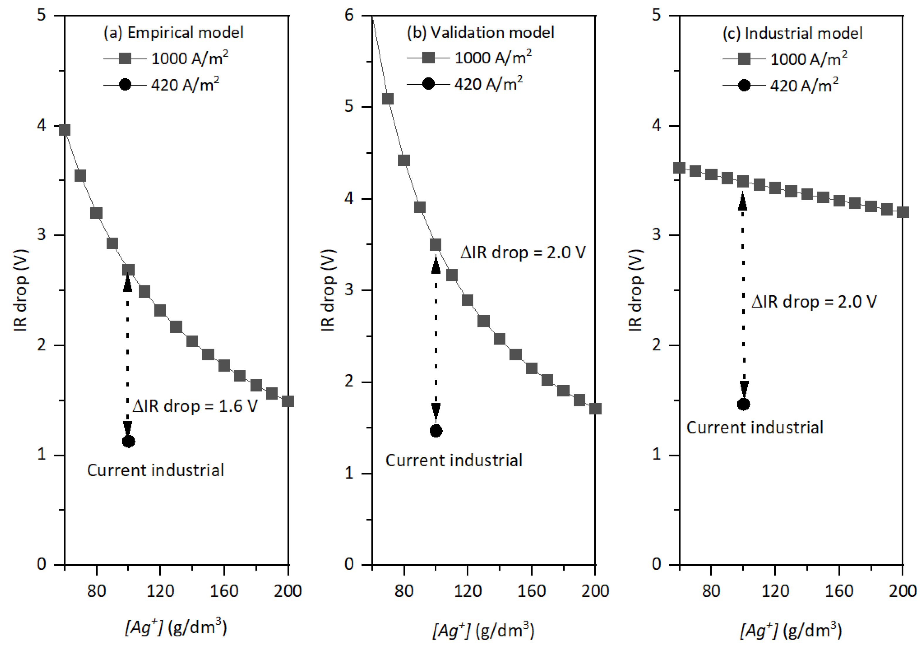
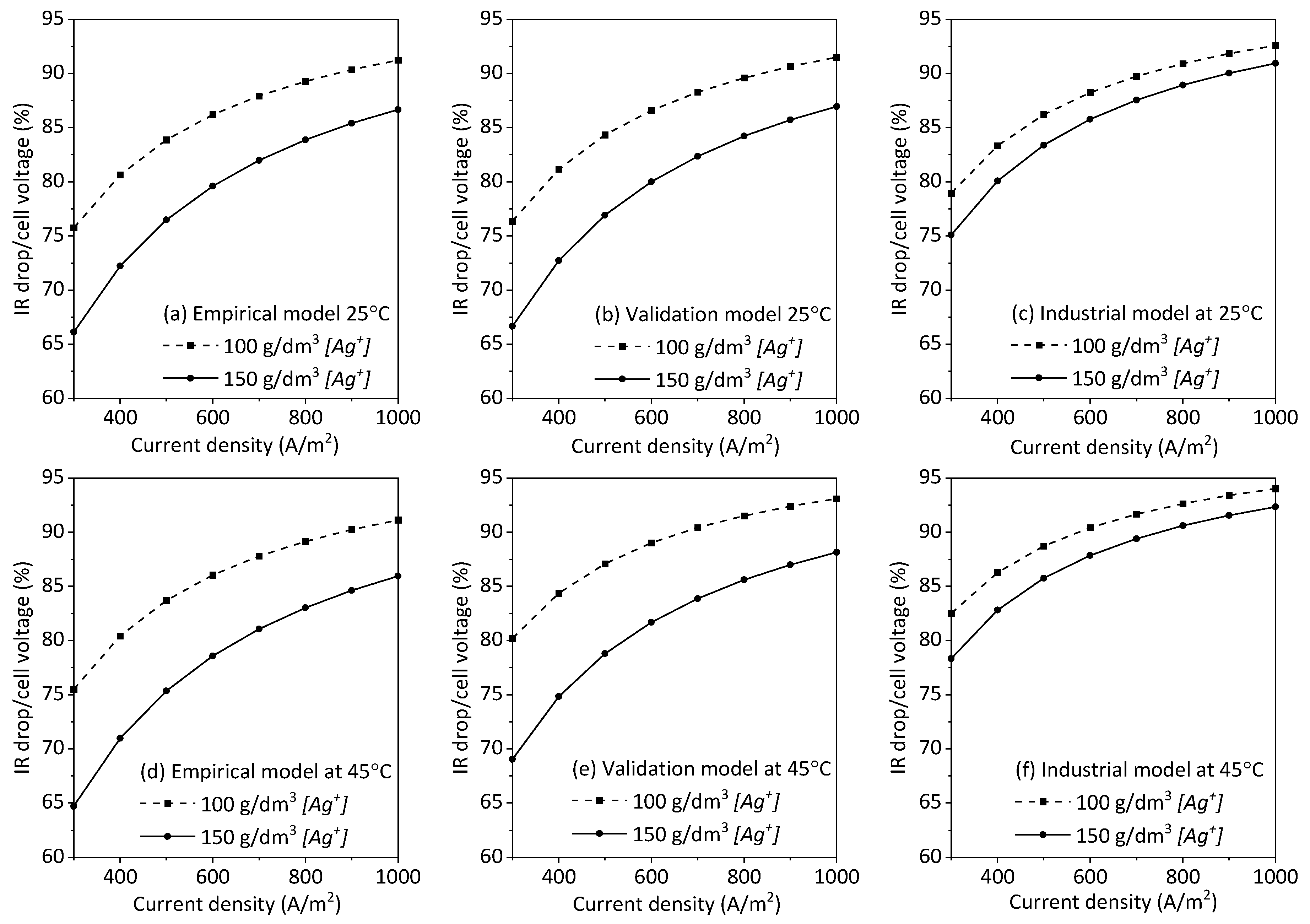
4.1. IR Rrop
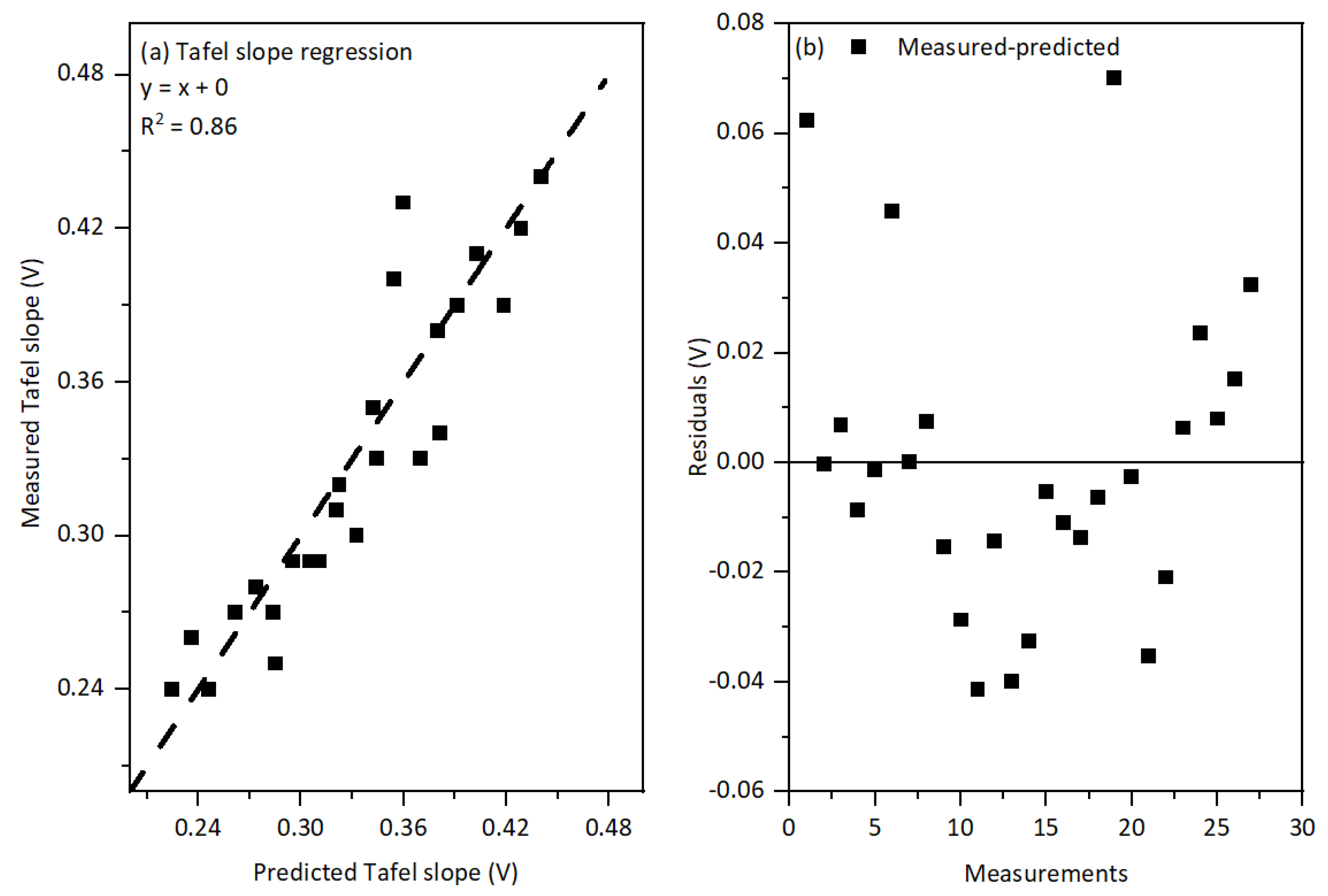
4.2. Anodic and Cathodic Overpotential (ηa and ηc)
4.3. Passivation Overpotential (ηpass)
4.4. Circulating Electrolyte volume
4.5. Cell Voltage, SEC, and Silver Inventory
- IR drop
- ○
- Empirical model = 2.05–2.75 V
- ○
- Validation model = 2.30–3.24 V
- ○
- Industrial model = 3.52–3.67 V
- ηa and ηc = 0.32–0.40 V
- ηAu = 0.02 V
5. Conclusions
Author Contributions
Funding
Conflicts of Interest
References
- Habashi, F. Handbook of Extractive Metallurgy: Volume III Part 6: Precious Metals; Wiley-VCH Verlag-GmbH: Weinheim, Germany, 1998. [Google Scholar]
- The Silver Institute. World Silver Surveys. Available online: https://www.silverinstitute.org/all-world-silver-surveys/ (accessed on 1 April 2020).
- Mostert, P.J.; Radcliffe, P.H. Recent advances in gold refining technology at Rand Refinery. Dev. Miner. Process. 2005, 15, 653–670. [Google Scholar] [CrossRef]
- Maliarik, M.; Johansson, K.Å.; Ögren, B.; Berg, G.; Johansson, C.D.; Lindh, R.; Ludvigsson, B. High current density silver electrorefining process: Technology, equipment, automation and Outotec’s Silver Refinery Plants. In Proceedings of the 7th International Symposium of Hydrometallurgy, Victoria, BC, Canada, 22–25 June 2014; Volume 2, pp. 91–100. [Google Scholar]
- Jaskula, M.; Kammel, R. Untersuchungen zur Verbesserung des Platinmetalausbringens bei der industriellen Silberraffination. Metall 1997, 51, 393–400. [Google Scholar]
- Pophanken, A.K.; Friedrich, B.; Koch, W. Challenges in the Electrolytic Refining of Silver–Influencing the Co-Deposition through Parameter Control. Rare Metal Technol. 2017, 2, 327–380. [Google Scholar]
- Leigh, A.H. Precious metals refining practice. In Proceedings of the 2nd International Symposium on Hydrometallurgy, Chicago, IL, USA, 25 February–1 March 1973; pp. 95–110. [Google Scholar]
- Pletcher, D.; Walsh, F.C. Industrial Electrochemistry, 2nd ed.; Springer: Dordrecht, The Netherlands, 2012; pp. 238–242. [Google Scholar] [CrossRef]
- Cornelius, G. Die Raffination von Gold und Silber durch Elektrolyse. In Elektrolyse der Nichteisenmetalle: 11. Metallurgisches Seminar GDMB; Verlag Chemie: Weinheim, Germany, 1982; Volume 37, pp. 215–226. [Google Scholar]
- Shibasaki, T.; Tsubogami, H.; Nozaki, M. Recent Improvements in Silver Electrolysis at Mitsubishi’s Osaka Refinery. In Proceedings of the Precious Metals’89, TMS conference, Las Vegas, NV, USA, 27 February–2 March 1989; pp. 419–430. [Google Scholar]
- Mantell, C.L. Industrial Electrochemistry, 2nd ed.; McGgraw-Hill: New York, NY, USA, 1940; pp. 253–254. [Google Scholar]
- Brumby, A.; Braumann, P.; Zimmermann, K.; van den Broeck, F.; Vandevelde, T.; Goia, D.; Renner, H.; Schlamp, G.; Zimmermann, K.; Weise, W.; et al. Silver, silver compounds, and silver alloys. In Ullmann’s Encyclopedia of Industrial Chemistry; Wiley-VCH Verlag GmbH & Co. KGaA: Weinheim, Germany, 2012; pp. 42–43. [Google Scholar]
- Aji, A.T.; Kalliomäki, T.; Wilson, B.P.; Aromaa, J.; Lundström, M. Modelling the effect of temperature and free acid, silver, copper and lead concentrations on silver electrorefining electrolyte conductivity. Hydrometallurgy 2016, 166, 154–159. [Google Scholar] [CrossRef]
- Aji, A.T.; Aromaa, J.; Wilson, B.P.; Mohanty, U.S.; Lundström, M. Kinetic Study and Modelling of Silver Dissolution in Synthetic Industrial Silver Electrolyte as a Function of Electrolyte Composition and Temperature. Corros. Sci. 2018, 138, 163–169. [Google Scholar] [CrossRef]
- Aji, A.T.; Halli, P.; Guimont, A.; Wilson, B.P.; Aromaa, J.; Lundström, M. Modelling of silver anode dissolution and the effect of gold as impurity under simulated industrial silver electrorefining conditions. Hydrometallurgy 2019, 189, 105105. [Google Scholar] [CrossRef]
- Aji, A.T.; Aromaa, J.; Lundström, M. Specific Energy Consumption Modelling of Silver Electrorefining. In Proceedings of the European Metallurgical Conference (EMC), Dusseldorf, Germany, 23–26 June 2019; Volume 2, pp. 807–820. [Google Scholar]
- Gordon, N.L.; Davenport, W.G. Electrical conductivities, densities and viscosities of silver refining electrolyte. Can. Min. Q. 1981, 20, 369–372. [Google Scholar] [CrossRef]
- Maurell-Lopez, A.K. Verhalten von Kupfer und Palladium bei der Raffinationselektrolyse von Recycling-Silber; Shaker Verlag GmbH: Düren, Germany, 2017; ISBN 978-3-8440-5987-8. [Google Scholar]
- Johnson, O. Refining processes. In Silver: Economics, Metallurgy, and Use; Butts, A., Coxe, C.D., Eds.; Van Nostrand Company, Inc.: Princeton, NJ, USA, 1967; Chapter 5. [Google Scholar]
- Hunter, W. Electrolytic Refining. US Patent no. 3,975,244, 17 August 1976. [Google Scholar]


| Parameters | [1] | [5] | [6] | [7] | [8] | [9] | [12] |
|---|---|---|---|---|---|---|---|
| [Ag+] | 50 | 150–200 | 65–120 | 150 | 30–150 | 50 | 50 |
| [HNO3] | 10 | 2.5 | 0.6–10 | 2–6.2 * | 0–10 | - | 10 |
| T (°C) | - | 35–50 | 35 | 32 | 25 | 45 | - |
| wt%Ag (%) | 95 | 99.3 | 96.5 | 86–92 | 86–92 | 98 | ˃ 99 |
| wt%Au (%) | 4 | 0.04–0.07 | 0.01 | 8–9 | 8–9 | 0.5 | - |
| wt%Cu (%) | 1 | 0.4–0.6 | 3 | 0.5–1 | 0.5–1 | 1 | - |
| j (A/m2) | 400–500 | 1000 | 500–800 | 300 # | 200–400 | 400 | 400–500 |
| Vcell (V) | 2.0–2.5 | - | - | 2.7 | 1.5–2.8 | - | 2.0–2.5 |
| Parameters | [Ag+], g/dm3 | [HNO3], g/dm3 | [Cu2+], g/dm3 | [Pb2+], g/dm3 |
|---|---|---|---|---|
| Values | 97.9 ± 8.3 | 0.3 ± 0.1 | 56.9 ± 1.9 | 1.6 ± 0.1 |
| Concentrations | [19] | [7] | [20] | [6] | |
|---|---|---|---|---|---|
| [Ag+] | 40 | 150 | 60–160 | 65–120 | ˃ 60 |
| [Cu2+] | 35 | max 45 | 60 | max 50–100 | < 60 |
| [Cu2+]/[Ag+] | 0.875 | 0.3 | 0.5–1 | 0.77–0.83 | 0.8–1.3 |
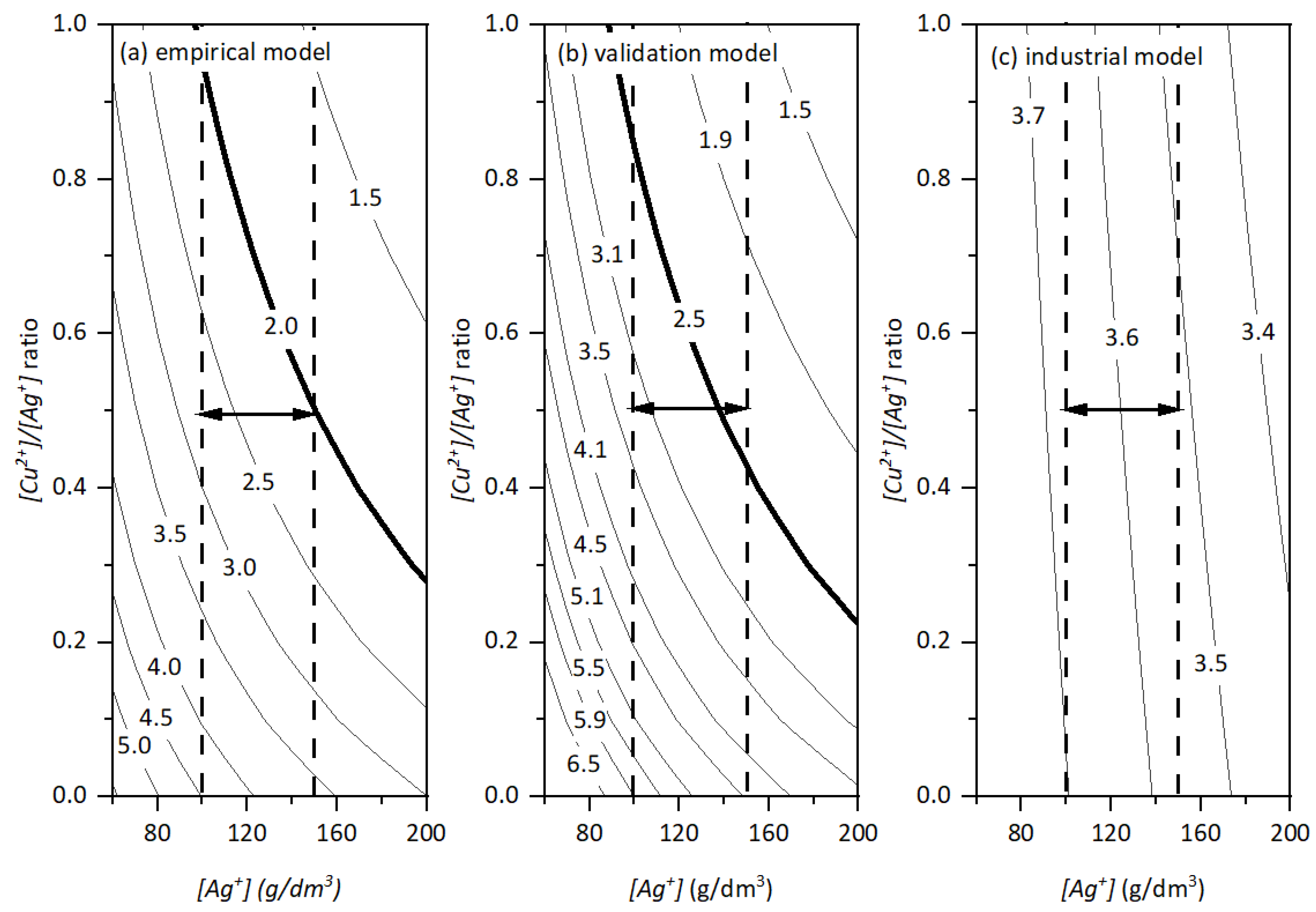
| Level | [Ag+], g/dm3 | Optimum [Cu2+]/[Ag+] | [Cu2+], g/dm3 | IR Drop (V) | ||
|---|---|---|---|---|---|---|
| Empirical | Validation | Industrial | ||||
| Min [Ag+] | 100 | 0.5 | 50 | 2.75 | 3.24 | 3.67 |
| Max [Ag+] | 150 | 0.5 | 75 | 2.05 | 2.30 | 3.52 |
| Parameters | HCD in This Study | HCD from Previous Study [4] | Conventional Silver Electrorefining [7,8,9,10,11,12] |
|---|---|---|---|
| [Ag+] (g/dm3) [Cu2+] (g/dm3) [HNO3] (g/dm3) T (°C) | 100–150 50–75 5–7 35–45 | 100–150 n.a n.a <55°C | 30–150 45–100 0–10 25–50 |
| Current density (A/m2) | 1000 | 1000 | 200–500 |
Cell voltage (V)
|
| <5 V | 1.5–2.8 |
| Current efficiency (%) | 98–99 [4] | 98–99 | 92–95 |
SEC (kWh/kg)
|
| 1.27–1.28 * | 0.44–0.76 |
| Comparisons based on 100 kg of Ag product / day | |||
| Electrolyte volume (dm3) Silver inventory (kg) | 259 25.9–38.85 | 259 * 25.9–38.85 * | 518–1295 * 15.54–194.25 * |
Publisher’s Note: MDPI stays neutral with regard to jurisdictional claims in published maps and institutional affiliations. |
© 2020 by the authors. Licensee MDPI, Basel, Switzerland. This article is an open access article distributed under the terms and conditions of the Creative Commons Attribution (CC BY) license (http://creativecommons.org/licenses/by/4.0/).
Share and Cite
Aji, A.T.; Aromaa, J.; Lundström, M. The Optimum Electrolyte Parameters in the Application of High Current Density Silver Electrorefining. Metals 2020, 10, 1596. https://doi.org/10.3390/met10121596
Aji AT, Aromaa J, Lundström M. The Optimum Electrolyte Parameters in the Application of High Current Density Silver Electrorefining. Metals. 2020; 10(12):1596. https://doi.org/10.3390/met10121596
Chicago/Turabian StyleAji, Arif T., Jari Aromaa, and Mari Lundström. 2020. "The Optimum Electrolyte Parameters in the Application of High Current Density Silver Electrorefining" Metals 10, no. 12: 1596. https://doi.org/10.3390/met10121596
APA StyleAji, A. T., Aromaa, J., & Lundström, M. (2020). The Optimum Electrolyte Parameters in the Application of High Current Density Silver Electrorefining. Metals, 10(12), 1596. https://doi.org/10.3390/met10121596