Article

Sensitivity Analysis in the Modelling of a High Speed Steel Thin-Wall Produced by Directed Energy Deposition

by
Rúben Tome Jardin
1,
Víctor Tuninetti
2,*,
Jérôme Tchoufang Tchuindjang
3,
Neda Hashemi
3,
Raoul Carrus
4,
Anne Mertens
3,
Laurent Duchêne
1,
Hoang Son Tran
1 and
Anne Marie Habraken
1,5,*
1
Department ArGEnCo-MSM, University of Liège, Quartier Polytech 1, allée de la Découverte 9, 4000 Liège, Belgium
2
Department of Mechanical Engineering, Universidad de La Frontera, Francisco Salazar 01145, Temuco 4780000, Chile
3
Department A&M–MMS, University of Liège, Quartier Polytech 1, allée de la Découverte 9, 4000 Liège, Belgium
4
Sirris Research Centre (Liège), Rue Bois St-Jean 12, 4102 Seraing, Belgium
5
Fonds de la Recherche Scientifique–F.R.S.-F.N.R.S., 1000 Brussels, Belgium
*
Authors to whom correspondence should be addressed.
Metals 2020, 10(11), 1554; https://doi.org/10.3390/met10111554
Submission received: 29 October 2020 / Revised: 17 November 2020 / Accepted: 19 November 2020 / Published: 22 November 2020

Abstract

:
This paper reports the sensitivity of the thermal and the displacement histories predicted by a finite element analysis to material properties and boundary conditions of a directed-energy deposition of a M4 high speed steel thin-wall part additively manufactured on a 42CrMo4 steel substrate. The model accuracy was assessed by comparing the simulation results with the experimental measurements such as evolving local temperatures and distortion of the substrate. The numerical results of thermal history were successfully correlated with the solidified microstructures measured by scanning electron microscope technique, explaining the non-uniform, cellular-type grains depending on the deposit layers. Laser power, thermal conductivity, and thermal capacity of deposit and substrate were considered in the sensitivity analysis in order to quantify the effect of their variations on the local thermal history, while Young’s modulus and yield stress variation effects were evaluated on the distortion response of the sample. The laser power showed the highest impact on the thermal history, then came the thermal capacity, then the conductivity. Considering distortion, variations of the Young’s modulus had a higher impact than the yield stress.

1. Introduction

Within the additive manufacturing (AM) processes, directed-energy deposition (DED) is a generic name for layered manufacturing of fully dense parts based on progressive welding of a wire or metal powder (Figure 1) on a substrate. The energy sources required for melting the feed metal in DED processes can be provided by electron beam (EB), laser (L), plasma, or electric arc. The most known DED processes are laser cladding (LC) or laser metal deposition (LMD) such as wire-based laser metal deposition (LMD-W) or powder-based laser metal deposition (LMD-P), electron beam melting (EBM) powder- or wire-based, plasma transferred arc (PTA) deposition, and wire arc additive manufacturing (WAAM) processes such as gas tungsten arc welding (GTAW) or gas metal arc welding (GMAW).
The main advantages of DED processes compared to powder bed fusion (PBF) processes (laser (L-PBF) or electron beam (EB-PBF)) are their high versatility and controllability. They can be used for manufacturing new parts, including directional solidification or single crystal cases, for adding features to existing parts, and for functionally graded parts [1]. DED is often used to provide an effective and minimally invasive approach, preventing the replacement of price-sensitive products [2]. Its use in repair operations receives increasing interest in industry [3,4,5]. Production of functional prototypes is another market, alongside production of small series. The variation of powder composition and the process parameter windows allow a tight control of chemical composition, melt pool size, thermal gradients, and solidification rates to control the generated microstructures [6]. Predicting and adapting the temperature distribution in parts produced by additive manufacturing processes are the basis for preventing distortion, residual stresses, and microstructural phenomena. To this end, Graf et al. [7] performed numerical analysis to determine the influence of wire feed rate and weld path orientation on the temperature evolution of multilayered steel and magnesium alloy walls manufactured by cold metal transfer (CMT) technology, a new form of gas-metal arc-welding process. Kiran et al. [8] focused on developing an adapted weld model for DED simulations of parts’ size between centimeters and 1 meter with a cost-efficient computational time. According to their results, the so-called thermal cycle heat input reduces the computational time considerably but some limitations with transient heat input model are still required. Manufacturing defects such as low forming precision, coarse grains, and pores caused by local heat accumulation can be mitigated with vortex online cooling [9]. Aldalur et al. [10] reported the use of oscillatory strategy for building a wall geometry with gas metal arc welding, resulting in an improved flatness and quasi-symmetrical geometry with a more homogenous microstructure than the overlap strategy. Despite these improvements, many issues are still to be mastered such as geometry accuracy and microstructure monitoring and control. Crack events during the manufacturing process or during cooling stage either at substrate-deposit interface or in the clad can also be an issue.
In order to be cost efficient and avoid expensive experimental work, different models can be applied. Pinkerton’s review paper [11] lists two types of model trends: the empirical-statistical models and the physical models devoted to powder flow, melt pool, microstructure, stress, distortion, or geometry. This article confirms that finite element (FE) analyses can be used to predict the thermal history and the distortions during the process, as well as the residual stresses or the microstructure at any material point. This quite extensive review [11] presents the current low level of knowledge about the DED models related to high-speed steel with their complex microstructure, while titanium alloys or superalloys have been extensively studied. It reminds also that non-equilibrium material state present in DED process prevents easy use of classical continuous cooling transformation diagrams.
The simulation targets usually define the model scale. For instance, to prevent balling effect and understand pore formation, detailed melt pool modeling and fluid simulations cannot be avoided. Note that with such a fluid methodology, in DED, Khairallah et al. [12] explains the flaw mechanism for both stainless steel 316L and nickel-based superalloy IN738LC, while Heeling et al. [13] presents the optimization of the process parameters for stainless steel. However, the micro scale of these models prevents them from addressing the simulations of whole parts, while even lower scale and other types of models, for instance, phase field approach [14,15], would be required to analyze the segregation behavior and the generation of phases. As explained by Jardin et al. [16], the precipitation of the carbides within M4 cladding results in a heterogeneous distribution of the carbide shape, size, and nature along the depth of a cladded sample. A phase field model is a further step for University of Liège team. Another example of the interest of low-scale method is the study of the diffusion between Si inclusions and Al matrix for AlSi10Mg determining the rupture location [17].
At the macroscopic scale, more adapted to industrial parts, the inherent strain-based method [18] is often used. It assumes incompatible strains from different sources and decouples stress components. However, the accuracy of this method for complex parts is not guaranteed and a careful calibration is always required either based on direct experiments or based on a detailed validated simulation. Detailed FE simulations close to the physical phenomena is this paper’s scope. It provides a deeper understanding of the material history within the process and helps to identify its control parameters. However, those simulations still present computer’s central processing unit (CPU) issues, which limit them to simple parts. As demonstrated hereafter, the mechanical result accuracy is not guaranteed for complex material as M4 steel deposited on 42CrMo4 substrate.
As the thermal field is the key factor, numerous 2D and 3D FE simulations at the macroscopic scale have been developed for academic samples providing the thermal history of deposits. For instance, special focus on the heat-affected zone is chosen by Yang et al. [19], while the effect of the laser scanning speed on the thermal evolution and on the melt pool size is studied by Patil and Yadava [20], of laser power by Yin et al. [21], and of preheating temperature by Chiumenti et al. [22]. However, those previous works do not discuss the impact of the accuracy of the input material parameter data on their predictions. Often by lack of knowledge, strong simplifications are done. A common simple assumption is to neglect the variations of the thermophysical properties with the temperature [23] or adopting constant heat convection coefficient for the boundary conditions [24], while the variation of this coefficient with the geometry and the temperature was demonstrated by [25]. The shape of the heat input developed by Goldak’s work [26], intended to model the laser beam heat source, could be used. However, a constant local value of heat input or a simplified shape is often adopted [27,28].
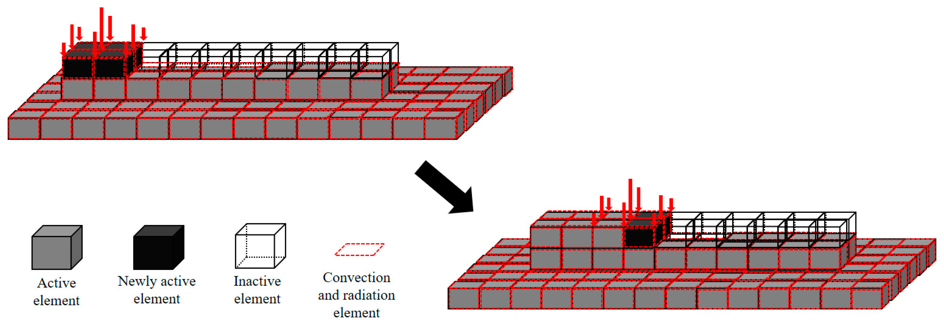
Another cutoff from the complex physics concerns the geometry of the added material at each track within a new layer of added material. By convenience, it is often a cuboid volume related to mean size of the track height and the track width. Within thermomechanical solid FE simulations, only some models like the one of Lindgren et al. [29] compute the added volume shape based on physical assumptions. Another way was chosen by Caiazzo et al. [30], who define it by regression formulas based on an extensive experimental campaign.
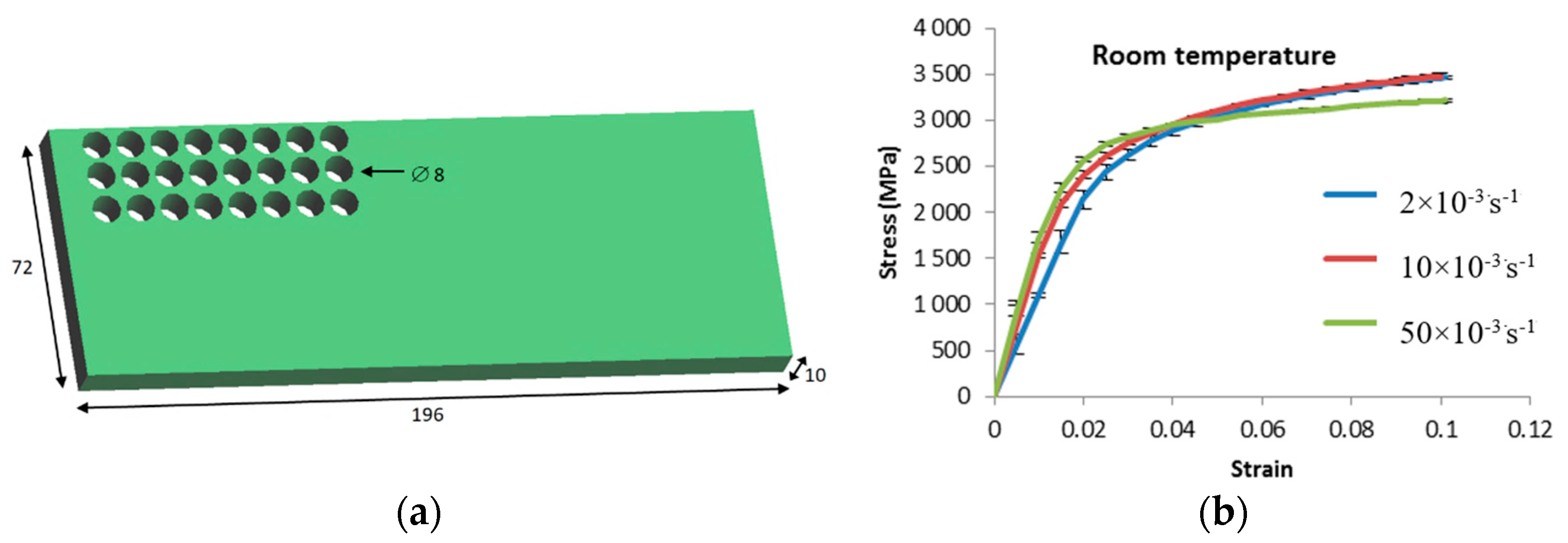
Key material information such as visco-plastic behavior within the mechanical model is usually based on experimental measurements from samples not manufactured by DED [29]. However, as pointed out by Lu and his coworkers [31], this approach is not reliable to generate accurate predictions as mechanical and thermophysical properties strongly depend on microstructures that are different in casting, forging, or additive manufacturing processes. The sensitivity analysis of Lu et al. [31] about the effect of mechanical properties of Ti-6Al-4V alloy shows that the distortion and residual stresses strongly depend on the values of the thermal expansion coefficient and the elastic limit, while slightly on the Young’s modulus.
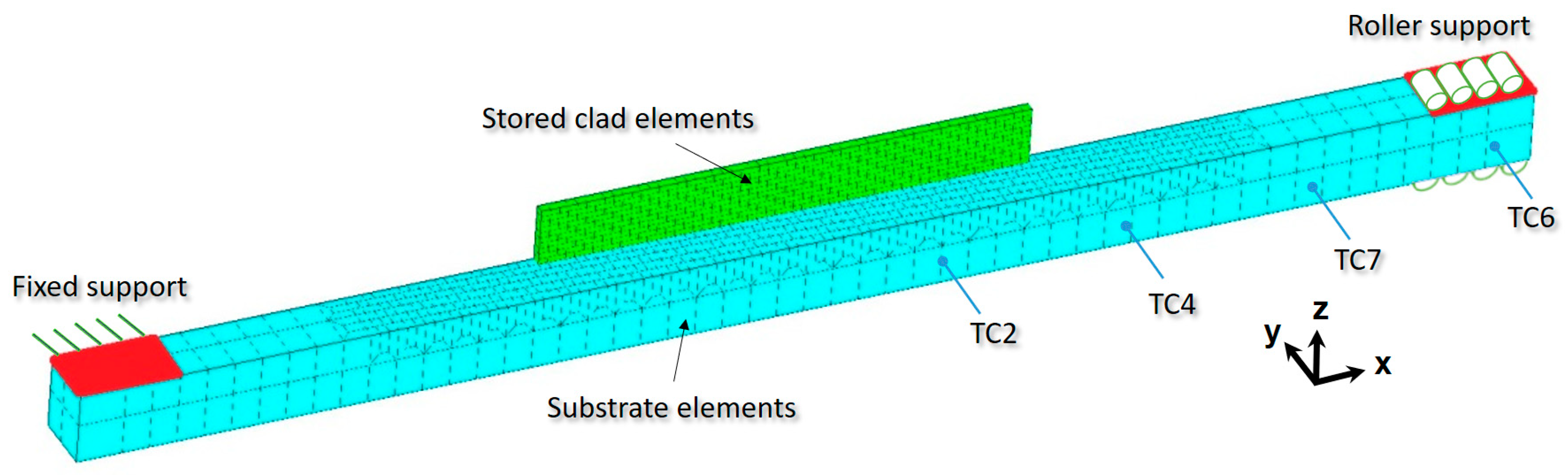
The present research focused on a thin-wall sample of 10 layers of M4 material on a substrate in 42CrMo4 steel. Thermomechanical finite element simulations compute thermal history of the cladded material as well as distortion and local temperature of substrate. As shown next, the access to accurate material data for this specific high-speed steel (HSS) grade is more problematic than CPU issues. A thorough validation of the model results was conducted using the predicted displacement and temperature curves of different points in the material, which were compared with their corresponding measured values throughout the process, including substrate preheating, deposition, and cooling. Final microstructure was measured by optical and scanning electron microscopy performed at the middle cross-section of the thin wall and substrate for further correlation analysis with the thermal history. Note that M4 material was selected because of its enhanced performances in wear and hardness when manufactured by DED [32,33]. However high amount of carbon in the material composition combined with thermal and/or phase-transformation stresses generates a high susceptibility to crack formation [34,35]. This feature explains why DED of tool steels remains very challenging. In addition to the usual process parameters, such as laser power, scanning speed, powder flow rate, and scanning strategy (laser path, idle time, track interdistance), the identification of the preheating temperature level is a mandatory step.
The cracks easily appear due to the tensile stress generated in the clad bottom or at the clad–substrate interface during the cladding process. The preheating temperature of the substrate decreases the space thermal gradient and the cooling rate and minimizes the thermal distortions and stresses during the process. As shown by Leunda et al. [36] for CPM 10V and Vanadis 4 extra tool steel powders, the crack appearances can be avoided by a preheating temperature below the maximum tempering temperature. For M4 powder, Shim et al. [32] specifically analyzed the effects of the substrate preheating on the metallurgical and mechanical characteristics of the manufactured parts. The results enhanced the effect of the preheating on the cooling history and solidification rates. Specimens without preheating mainly include equiaxial fine grains, whereas the induction-heated specimens generate columnar grains. However, no significant hardness differences were measured, which could be explained by secondary hardening mechanism caused by hard and stable carbides. As pointed by Jardin et al. [16], for a preheating of 300 °C and a 36-layer clad of 40 × 40 × 27.5 mm3 (a bulk sample compared to the thin-wall geometry studied here) a strong heterogeneity appears within the clad deposit due to different thermal histories. Close to the deposit-free surface and at mid-height, the angular-like vanadium-rich metal carbides (MC) precipitated in intercellular zones just after the primary cells. The high superheating temperature within the melt pool at mid-height of the deposit promotes the coarsening of the solidification phases including cells and intercellular carbides. At intermediate depth of 4.5 mm from the deposit-free surface, a lower superheating temperature and a higher number of remelting of the material points promote the precipitation of coral-like vanadium-rich MC carbides inside cells.
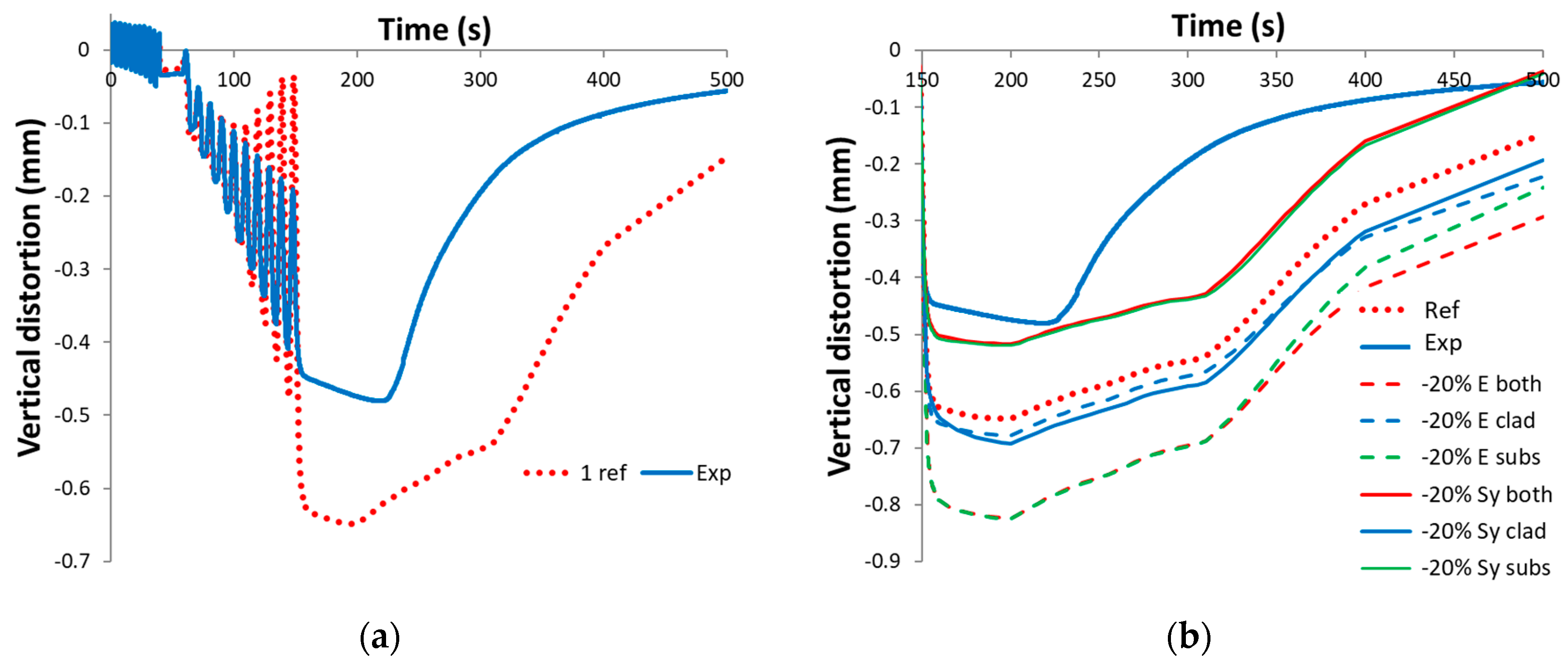
The present article aimed to quantify the variation of the numerical predictions due to different material properties such as stress–strain relationship, thermophysical variables, or boundary conditions such as convection and radiation flow. The prediction of distortion currently achieved lacks precision when compared with experimental results. However, forthcoming work on improving predictions, reducing residual stress, and increasing microstructure homogeneity will be based on numerical optimization. The complexity of the multiphase materials of both the clad and the substrate demonstrates that the model sensitivity analysis presented in this work is a required stage for obtaining reliable results.
The paper describes the thin-wall experiment in Section 2.1, the metallographic observations in Section 2.2, and the FE model in Section 2.3. The results of the material data measurements are provided in Section 3.1 and 
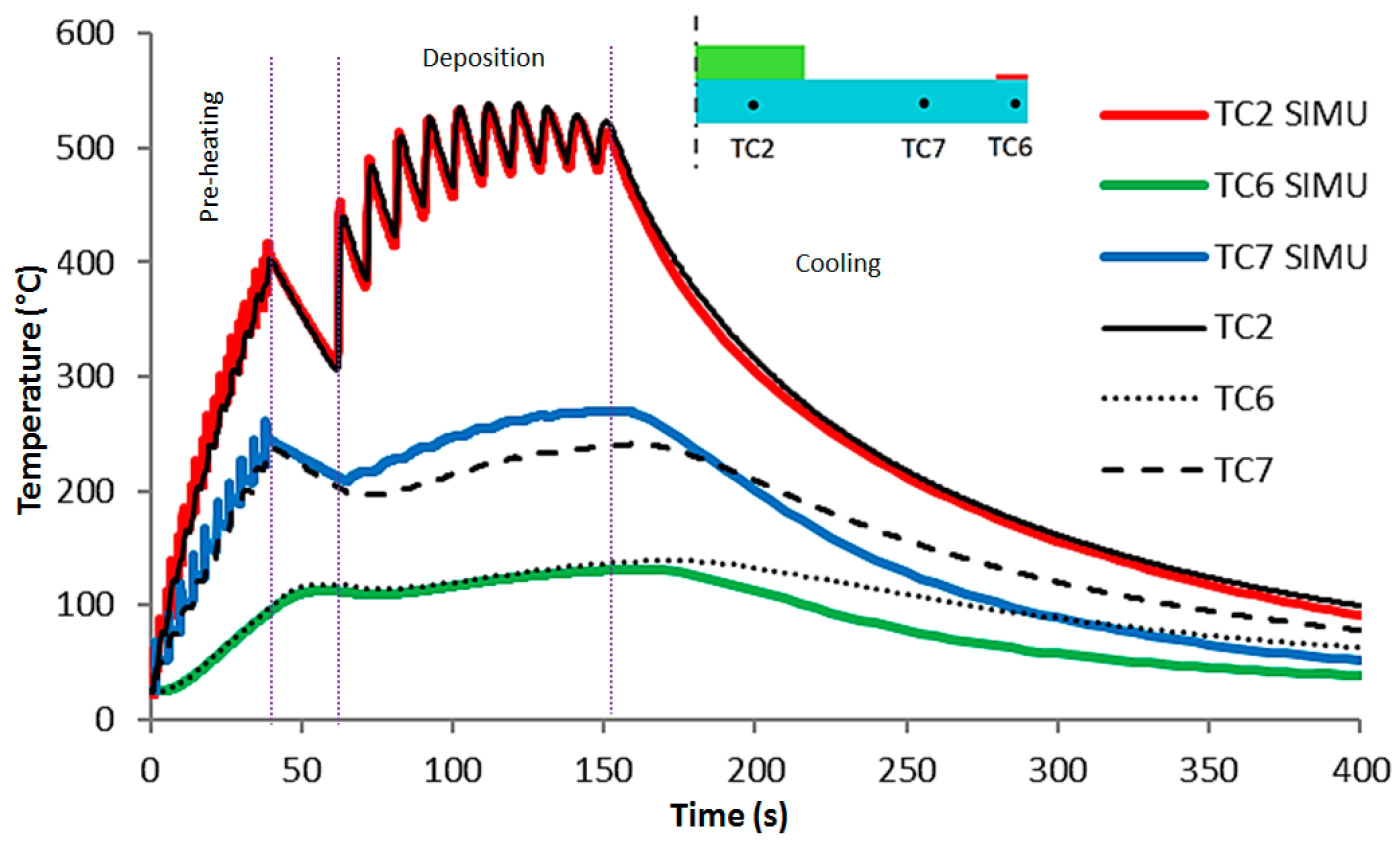
Section 3.2. The validation of the model was performed through a comparison between thermal history predictions of the substrate with experimental results in Section 4.1. In 
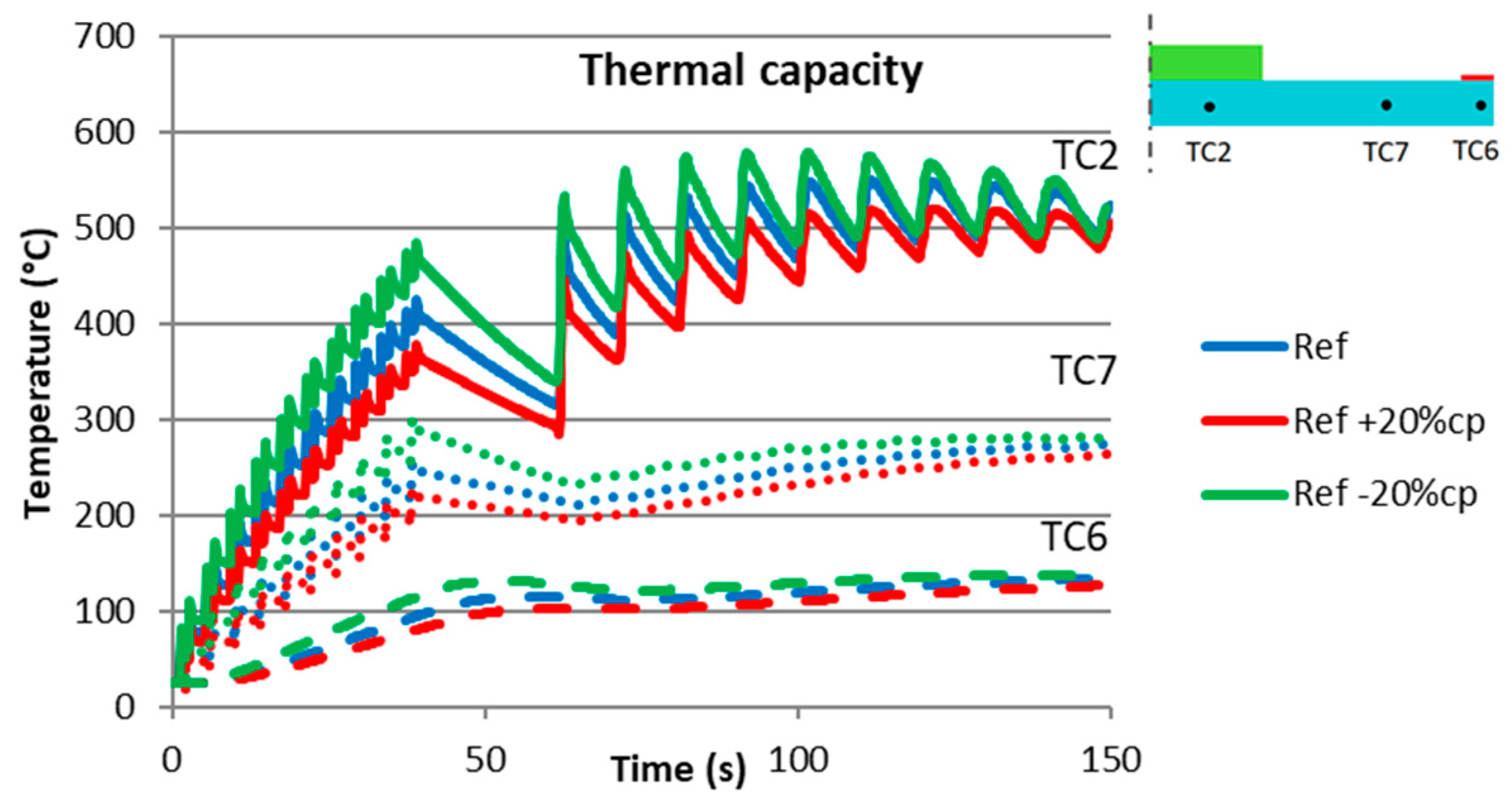
Section 4.2, the observed microstructure by optical microscopy (OM) and scanning electron microscopy (EM) is explained based on the predicted thermal history of the clad. The thermal and thermomechanical sensitivity analyses and discussions are given in Section 4.3 and Section 4.4, respectively. Finally, Section 5 provides the summary of the key results and the perspectives for ongoing research.

2. Materials and Methods

2.1. Thin-Wall Experiments

The composition of the HSS M4 commercial powder with its particle size ranging from 50 µm to 150 µm is provided in Table 1. The 5-axis Laser Cladding system (IREPA LASER, Ilkirch, France) with a Nd-YAG laser of maximum power capacity of 2000 W from Sirris Research Centre (SIRRIS, Seraing, Belgium) is schematically described in Figure 1. The laser has a wavelength of 1064 µm and operates continuously. The metal powder is injected with an angle of 45 degrees. The laser has a top-hat energy distribution with a mean diameter of 1500 µm (1400 µm at the top and 1600 µm at the bottom). The substrate consists of a small, rectangular bar of 8 mm height, 10 mm width, and 120 mm length of 42CrMo4 steel (Figure 2b). The bar supports are shown in Figure 2b while the thermocouple (TC) positions are given in Figure 2c. The preheating to prevent the crack appearance in the deposit was performed by preliminary laser passes (red line in Figure 2c). Preheating temperature values from 217 °C to 400 °C were generated. For the lowest preheating temperature, cracks appeared during the deposition of the fifth layer at the extremities of the substrate–clad interface (Figure 2a), but when manufactured with a preheating of 400 °C sound samples were achieved (Figure 2d). Table 2 gives the process parameters of the simulated manufacturing cases. The final manufactured thin walls of 40 × 4 × 1.5 mm3 were centered on the substrate top surface.

2.2. SEM and OM Metallographic Observations

The samples were mirror polished with oxide-based polishing suspension (OPS) finish, followed by etching with Vilella’s reagent. Figure 3 shows the cross-section observations of the sample obtained by optical microscopy (BX-60 M, Olympus Corp., Tokyo, Japan) and scanning electron microscopy (FEG-ESEM XL30, Philips, Eindhoven, The Netherlands). Optical microscopy (OM) images show a dark region of the deposit in the lower layers, except for the junction area, and a lighter region at the top, specifically in the last two layers. The fine precipitates in the dark areas are not present in the light areas, as observed in the scanning electron microscopy (SEM) images. Both zones show a cellular-type microstructure with eutectic carbides in the cell junctions, as already demonstrated in bulk deposits after manufacturing [16] or after tempering [33]. The matrix is of the martensitic type with eventual zones of residual unprocessed austenite, as already observed in a similar alloy [37].

2.3. Finite Element Model

The coupled thermomechanical simulations were performed using LAGAMINE code, a finite element software developed at the University of Liège in 1985. It has already been applied on many material-forming processes. The FE results of Pascon et al. [38] predicted the crack events in a continuous casting process. Neira Torres et al. [39] studied the manufacturing of bimetallic rolling mill rolls and computed residual stress state validated by X-ray diffraction. Guzmán et al. [40] simulated incremental sheet forming and focused on the geometry and force predictions with comparison with test measurements.
In Tran et al. [28], a 3D thermal simulation of DED of Ti6Al4V alloy with microstructure predictions validated by a measured hardness distribution map and microscopic observations was presented. In the present work, an extension of this model to mechanical analysis was used where temperature and displacement fields were simultaneously computed within an implicit strategy. Note that other thermomechanical FE models like the ones of Mukherjee et al. [41] or Chew et al. [42] apply sequential analyses where the thermal field is assessed in a first stage and applied as static load during the mechanical analysis defining the second step of the model. As the final goal was to reach a complete thermomechanical-metallurgical model, this staggered solution was not selected to prepare the future steps where all the couplings will be taken into account as the phase transformation key temperature can be strongly impacted by mechanical stresses.
However, currently only thermomechanical simulations are performed. The lack of material data prevents the activation of the coupled thermomechanical-metallurgical module able to predict kinetic of solid phase transformations, like in previous research [39]. Currently, the thermal expansion coefficients used for the clad and the substrate take into account phase transformation events through a multilinear curve, depending on temperature. The latter is, however, not related to cooling, heating temperature rates, and phase distribution. Without a more accurate input, the measured displacement field could not be totally correctly predicted, as shown below. However, a reference case was defined to allow a sensitivity analysis. The material model of the clad and the substrate was elasto-plastic based on von Mises yield locus and multilinear tangent modulus for isotropic hardening. Young’s modulus, elastic limit, and isotropic plastic hardening are temperature dependent. Note that the set of associated tangent plastic moduli was kept constant for each curve. Besides, as low-viscosity effect was confirmed by the mechanical tests (Section 3), the strain hardening model was rate-insensitive.
The eight-node 3D brick (BWD3T) thermomechanical finite element implemented in the Lagamine code by Zhu et al. [43] was selected. The element is based on the nonlinear, three-field Hu-Washizu variational principle of stress, strain, and displacement [44,45,46] and uses a mixed formulation adapted to large strains and large displacements with a reduced integration scheme—only one integration point—and an hourglass control technique.
The FE solid model simplified the physics of all the phenomena present in the melt pool. The effect of the latent heat of the fusion (Lf) was integrated in the definition of the thermal capacity (cp), defining an apparent property. The effect of the fluid motion due to the thermo-capillary phenomenon (i.e., Marangoni flow) was not considered. Other solid studies just consider a multiplicative factor to enhance the conductivity value within the melt pool [42,47]. Such a factor varies, according to the research. For instance, Cao et al. [47] use a value of 3 for Ti6Al4V alloy while Bi et al. [48] use a value of 5 for iron-based martensitic stainless-steel METCO 42C, respectively. Initially for welding, Lampa et al. [49] suggested a value of 2.5 for an austenitic stainless steel. Hereafter, following the arguments of Lindgren et al. [29], no multiplicative factor was applied as it counteracts the energy distribution defined in the heat source model. Clearly, such assumptions are not independent of the powder laser absorptivity factor β, which is the current work numerically tuned within the simulations’ process to agree with the observed melt pool size and the measured thermal history.
A second simplification consisted of the energy distribution of the heat flow of the laser. While the model developed by Goldak defines a double ellipsoidal power density distribution [26], a simple circular Gaussian is often considered [27,50]. The model considered in this present research was even simpler: The mesh size was adapted to the laser spot radius. The clad finite cubic elements had a 0.75 mm width to model the laser top-hat energy distribution with a diameter of 1.5 mm. As only half of the process was simulated by symmetry, and the final clad volume modeled was 40.5 (length) × 0.75 (width) × 4 (height) mm3. Indeed, the mean height of the layers was measured and corresponded to 0.4 mm. The effect of the moving laser beam was taken into account by updating the laser input power within the affected nodes, based on the real velocity and the trajectory of the laser processing head.
The 3D mesh of the substrate presented a mesh refinement depending on the space position. Refined elements were defined near the clad in order to accurately model heat fluxes, while the substrate bottom was meshed coarsely. To generate an accurate mesh, transition refinement elements were used, as shown in Figure 4. The thermal boundary conditions of the model consisted of convection and radiation in all surfaces except the symmetry plane and the supports where heat is transferred by conduction. Figure 4 also shows the mechanical boundary conditions of fixed support and roller support at the end of the substrate bar.
The principle of the element birth technique modeling the addition of material within the process is shown in Figure 5 on a simplified mesh. When a new layer is created during the material addition process, a group of four solid elements for the complete sample width (two elements, by symmetry here) is activated with their boundary conditions. LAGAMINE software applies convection and radiation by interface elements that rely on classical thermal equations, as described in Tran et al. [28]. When the laser beam is ongoing, new solid elements are activated with their new convection and radiation surface elements around them, while the convection and radiation elements under the new solid elements are deactivated. The laser power is directly applied at the top nodes of the activated elements.
The concept of numerical annealing temperature (Tanneal) [51,52] from welding models was applied here. It seemed physically consistent to neglect any plastic strain performed at higher temperature than a well-chosen annealing temperature. In the finite element code, if the temperature of the material point (integration point within an element) is higher than Tanneal, the material will lose its hardening memory; this effect was taken into account by setting the equivalent plastic strain to zero. When the temperature of the material point falls lower than Tanneal, the material can harden again. For instance, several authors [25,31,53,54,55] exploited this approach in order to compute the stress field and perform a sensitivity analysis to this annealing temperature value. However, the sensitivity of the predicted displacement field was lower than that of the stress and it seemed not a key feature in the current validation. Three different annealing temperatures (527, 727, and 1027 °C) were investigated plus a case without annealing. It was observed that the annealing temperature had low impact on the thermomechanical model and, thus, a final temperature of 527 °C was used, as it led to faster convergence.
The thermal boundary conditions considered in the numerical simulations took into account an absorption factor β, which differed for the preheating step and the cladding one. Its values were, respectively, 0.65 and 0.4 and were adjusted to recover the thermal measurements. During the preheating, the surface was flat compared to the clad deposition, implying a better absorption of the laser energy and a higher absorption factor.

3. Material Parameters

3.1. Thermophysical Properties

The thermophysical properties of the clad samples (Figure 6) manufactured by DED and the substrate were measured by He pycnometry, dilatometry (density, ρ), differential scanning calorimetry (DSC) (thermal capacity, cp), and laser flash analysis (LFA) (thermal diffusivity, α) within a range from 20 to 1100 °C (Appendix A). LFA measurements were carried out by steps of 100 °C. For the clad material, latent heat was also measured by DSC up to 1410 °C and added to the thermal capacity cp (J/kg °C), defining an apparent heat capacity c p * (J/kg °C):
c p * = { L f T D T m + c p ,     i f   T D T T m     c p ,     o t h e r w i s e                      
where L f (J/kg) is the latent heat of fusion, T m (°C) is the starting melting point (solidus temperature), and T D (°C) is the ending melting point (liquidus temperature). Finally, the thermal conductivity k was obtained using the following equation:
k ( T ) = α ( T ) · ρ ( T ) · c p ( T ) .
The errors associated with the equipment (Accupyc 1340 Micromeritrics (Micromeritics Instrument Corporation, Norcross, GA, USA), DIL 402C Netzsch (Netzsch-Feinmahltechnick GmbH, Selb, Germany), DSC 404C Netzsch, LFA 427 Netzsch (Netzsch-Feinmahltechnick GmbH, Selb, Germany) and measurements were 3% for cp, 7% for k, and 2% for ρ.
To measure the enthalpy of melting, sigmoidal baseline type was used to determine the area of the peak (Figure 7). The accuracy of enthalpy measurements was about ±5%. The measured values were 1230 °C for T m , 1404 °C for T D , and 313 J/g for the area of enthalpy of melting, L f . The thermophysical data identified for M4 can be found as a function of temperature in the Appendix A. It is worth noting that the measured values are within the range of partial results given in [56] for M4 HSS.
The substrate properties first relied on previous tests performed on 42CrMo4 grade in bainitic-martensitic state. The used values in simulations were similar to values found in [57]. However, a closer look at the material certificate identified a pearlitic state, which justified the final use of properties reported in [58], similar to what was finally measured on the substrate (Figure 8) where phase transformation occurred. This modification was a mandatory point to be able by simulations to recover the thermal field measured during substrate preheating, showing the high sensitivity to thermophysical properties.
Thermal expansion coefficients of the clad and the substrate are key issues for distortions and the stresses related to thermal gradients. However, they should be measured in similar conditions as the ones happening in the process to provide correct values related to the real microstructure events. As non-equilibrium and heterogeneous thermal histories and microstructures are known to be present within M4 clad samples [16], the applied temperature-dependent coefficient should be not related only to temperature value. The transformations are affected by temperature heating and cooling rate and successive transformations vary the chemical composition of phases. Finally, the stress state is known to shift key temperature features. One should build the dilatation coefficients from knowledge related to the kinetics of transformations and representative experiments. Within the cladding process, the material is submitted to temperature rates up to 4750 °C/s during cooling, for instance, while the available measurements were limited to 200 °C/s cooling rate. This cooling rate is enough to achieve phase transformation without diffusion. Last but not least, the initial state of the sample affects the results. To be close to real values, samples were extracted from bulk samples manufactured by DED process (process parameters: laser power of 1160 W, nozzle speed of 462 mm/min, and powder flow of 86 mg/s). Dilatometry tests, for cooling down from 1200 °C to room temperature at 120 °C/s, provided martensite start (Ms) temperature (260 °C) and, for a cooling rate of 0.5 °C/s, bainite start (Bs) temperature (370 °C) was obtained. However, the microstructures were different between the thin walls and the bulk samples as bainitic, martensite, and residual austenite were not in the same proportions. So, extracted data (Figure 9 and Figure 10) were still not reliable as the tested samples were neither remelted (maximum temperature in dilatometer was 1100 °C, far from 1404 °C liquidus and superheating temperature experienced within the melt pool not reached) nor submitted to correct the cooling rate during the process. Note that the effect from the cooling ratio and stress state was actually not taken into account.
Finally, the thermal expansion measured on DED samples (Figure 9) and data found within the literature defined a basis to assume the curves plotted in Figure 10 used within the reference thermomechanical simulation.
Note that those thermal dilatation coefficients ( α ) follow the classical metallurgist definition of:
α ( T ) = ( 1 / L 0 ) ( L T L 0 ) / ( T   T 0 )
where L is the length, T is the temperature and index 0 means at room temperature.

3.2. Stress–Strain Curves

Compression tests of cylinders of 8 mm diameter and 10 mm height were carried out on HSS-grade M4 samples at different temperatures and different strain rates in order to determine the stress–strain curves. The tests were performed with a Schenck 400 kN machine, and a quad elliptical radiant furnace 4 × 2000 W was used for high-temperature tests. The compression samples were cut using wire electro discharge machine from a part of a bulk deposit produced by DED (see Figure 11a and manufacturing conditions defined in Section 3.1). Samples were tested at room, moderate, and high temperatures (20, 300, 500, 950 °C) and at different constant strain rates (2 × 10⁻³, 10 × 10−3, and 50 × 10−3 s−1). For each combination of temperatures and strain rate conditions a minimum of three samples was tested. Note that the very high elastic stiffness of the samples, compared with the press stiffness at moderate and high temperatures, often affects the axial displacement actually applied on the samples. This test feature must be taken into account to reach an accurate constant strain rate test. An approach based on a linear speed of the press plateau decreased the precision of the measured elastic limit. The methodology of Tuninetti et al. [59] was applied here to achieve a real constant strain rate and an accurate yield stress.
As shown in Figure 12, the effect of strain rate in the analyzed range (2 × 10⁻³ to 50 × 10−3 s−1) was not very significant. The highest strain rates showed the lowest hardening. This effect was more obvious at room temperature (Figure 11b). If the plastic range can be trusted, the Young’s modulus was not reliable in those compression tests. It was more a trend than an accurate characterization and its identification is explained in next paragraph. For the case at 950 °C just one sample was successfully tested. However, the stress–strain curve measured by Neira Torres et al. [39] on a similar composition and forged samples were in close agreement. Based on those results, the strain rate sensitivity can indeed be neglected in the DED simulations of this material. Within the Lagamine simulations, the mean curves for 2 × 10⁻³ s−1 strain rate described by multilinear segments for each measured temperature define the hardening law. The intermediate values were interpolated for any strain and temperature.
The value of 216.3 GPa for the Young’s modulus relies on grindosonic measurements at room temperature. At higher temperatures, the Young’s moduli measured by Neira Torres et al. [39] on high chromium steel heat-treated samples are used, and the heat treatments provided different phase percentages. This input database allows correcting nonreliable, experimental Young’s moduli of this research by a mixture law for the compressed samples. According to the observed microstructures of the bainitic bloc (Figure 11a) and of the martensitic thin wall (Figure 3), Figure 12d provides more of an evolution trend than an accurate characterization of the Young’s moduli with the temperature. For 42CrMo4 mechanical data, the simulations were based on the stress–strain curves provided by Habraken and Bouffioux [60].

4. Results and Discussion

4.1. Thermal History Validation and Potential Effect on Distortion

The laser absorption, convection, and radiation coefficients were inversely identified by using the Levenberg Marquardt approach (Table 3). The simulation results of local temperature for preheating, cladding, and cooling were compared to the measured values at the thermocouple points, showing good accuracy predictions (Figure 13). The obtained local temperature values in the substrate near the cladding were more accurate than those at more distant substrate points, especially during the cooling stage. These errors could affect the thermomechanical predictability of cladding distortion. However, by verifying the substrate mechanical boundary conditions (Figure 2 and Figure 4) and the low-temperature values at TC6 and TC7 (less than 200 °C), the performed analysis indicated that the effect of this error on the measured z-displacement can be neglected. This affirmation was investigated through extreme fixations’ conditions and with high extraction of heat in the left fixation part.

4.2. Metallurgic Validation

In Figure 14, red and blue shading zones give the range of temperature variations (maximum and minimum) after the last total remelting for material points belonging to the first and fifth layers, respectively. The purple line (minimum temperature reached during the deposition process) increases until a maximum value of 527 °C. This curve confirms that neither bainitic nor martensitic transformations occurred during the process time, according the Bs (370 °C) and Ms (260 °C) temperatures. When the laser processing was switched on, the matrix was austenitic. It was transformed totally or partially to martensite at the cooling stage when the laser was switched off.
As the solid matrix of a material point remains austenitic during the laser switch on period, once the temperature stays under the liquidus, a pseudo-isothermal annealing (PIA) period can be assumed. Such an approach is inspired from the work achieved on a Ti6Al4V alloy processed by DED [28]. For each material point, the PIA temperature is set as the average from all the temperature levels contained within the shading domain processing. This information helps to generate a simplified approach for microstructure predictions based on a similar way to what is achieved with time–temperature-transformation (TTT) diagrams.
In Figure 14, the material point history of the central point of the first layer (blue curve) presents a first maximum peak (2081 °C), then the peak values gradually decrease with successive layer deposition. The situation is different for an intermediate layer such as the fifth one. The first peak (2161 °C), slightly higher than within the first layer, increases when the upper layer (the sixth) is added (2248 °C). These increases are due to the phenomenon of heat accumulation. This material point of the fifth layer is melted a third time when the seventh layer is deposited, but at a lower temperature. According to this thermal computed history, layer number 1 melts twice, while layer number 5 melts three times. However, none of the recorded points show more than one peak within the solidification interval (liquidus–solidus range). In Jardin et al. [16], a study that focused on a bulk sample, it was established that temperature fluctuations in this solidification interval strongly modify the solidification structure. In particular, it generates a microstructure with intra-granular pseudo-primary carbides. For the studied thin wall, the cell structure is such that carbides are present only in the cell junctions (inter-granular carbides) and not in the cell core for any layer.
The superheating temperatures of the last complete melting (1825 °C, 1456 °C, and 1953 °C in layers 1, 5, and 10, respectively) and the cooling rates define the size of the primary grains and the cellular type solidification mode. The average size of the solidification cells shows a slight variation (see Figure 3), starting with a decrease between layers 1 and 5 and ending with an increase in the last deposit.
These observations are consistent with the solidification parameters experimentally observed: A cell refinement is favored by the very high cooling rate, the multiple remelting cycles, and overheating of the liquid metal (Figure 3, fifth layer).

4.3. Sensitivity Analysis of Thermal Response

This section evaluates the uncertainty of the model results caused by the effect of different error sources on input parameters such as power, thermal capacity, and conductivity. The evolution of temperature over time at the measurement points TC2, TC7, and TC6 were evaluated as a function of ±20% variations in the thermal capacity of the cladding and the substrate (Figure 15), the conductivity of the substrate (Figure 16), and the laser power (Figure 17) with respect to the values used in the validated reference simulation. Thermal histories computed for independent variations in either the conductivity or the heat capacity of the clad revealed an insignificant effect due primarily to the low mass of the thin-wall cladding compared to the mass of the substrate. The negligible effect of such variations is not shown and becomes considerable when bulk deposits are analyzed, as reported in [61].
Variations in the thermal capacity of the cladding and substrate significantly affect thermal history predictions (Figure 15). The largest temperature difference found with respect to the reference simulation was 16% at 27.4 s at the TC6 during the preheating stage. Increasing thermal capacity (cp) by +20% produced a decrease in temperature by approximately 12% during preheating, followed by a linear increase of up to 5% difference at the end of the deposition. On the other hand, a negative variation of 20% of cp generated a maximum temperature increase of 25% during substrate preheating stage, which then decreased linearly to 2% above the reference temperature at the end of the clad process. This asymmetric temperature behavior can be related to the interaction between conduction and heat accumulation, which makes the transient response nonlinear with respect to thermal capacity. Finally, the results demonstrated that overall temperature was asymmetrically and inversely proportional to the thermal capacity.
The sensitivity analysis of thermal history to conductivity (Figure 16) showed different trends. Here, the effect of the variation was mainly visible closer to the clad. The phenomena observed were expected because, with an increased conductivity, heat propagates more easily in the substrate. There is less heat concentration close to the deposit (hence, lower temperature), and far from the deposit there is more heat transmission before being lost by convection and radiation. Conversely, lower conductivity increases the temperature near the cladding zone because more heat is transferred from the free surface of the substrate to the environment. This latter behavior is consistent with the lumped heat capacity of the substrate, where internal resistance to heat transfer becomes negligible in comparison to the external resistance of convection and radiation. This fact also explains the small effect of conductivity on temperature variations at TC7 and TC6 points located far from the clad. From Figure 15 and Figure 16, it can be concluded that the thermal history of the thin wall of HSS is more sensitive to thermal capacity than to conductivity.
Global sensitivity analysis of power (Figure 17) on thermal history is self-explicative. Results show that increase in power leads to an increase of temperature and vice versa. Such high sensitivity helps to get an easy identification of absorption coefficient.

4.4. Sensitivity Analysis of Thermomechanical Response

The identified evolution of thermal expansion coefficients of the clad and the substrate (Figure 9 and Figure 10) are essential and highly influential for determining the behavior of deformation and stress fields. However, these coefficient values strongly vary with the phase transformation kinetics of both materials. The impact of these phase transformations was not assessed in this article, as that would necessitate the need to include a metallurgical model. Currently, metallurgical data and models for very high heating and cooling rates for high speed steel are lacking. Thus, in a pragmatic exploratory research, the assumed average thermal expansion curves of Figure 10 were kept the same and just the impacts of the Young’s modulus and the yield stress accuracy were investigated.
The predicted vertical displacements of the substrate bottom point at mid-length (zz sensor at Figure 2b) were compared with their measured values (Figure 18a) during the preheating, deposition, and cooling processes. Figure 18b shows the sensitivity analysis of the elastic modulus (E) and initial yield stress (Sy) on this displacement during the cooling stage. Note that the elastoplastic behavior of the material was based on a multilinear isotropic hardening law, taking into account both temperature dependence of the Young’s modulus and the initial yield stress. The hardening shape defined for each temperature was not modified. The FE predictions were in close agreement with the measured values (Exp) for both the preheating and the first five deposition stages (Figure 18a). Note that three similar experiments were performed with low scattering. The mismatch can be related to the microstructure transformations happening within the first layers as their temperature was low enough to reach solid-state transformation zones. A zoom on the process’ last stage, the cooling, is shown in Figure 18b.
It has been numerically checked that, within preheating and deposition stages, the effect of Young’s modulus and yield stress variations were not significant. For this reason, the sensitivity analysis was limited to the cooling stage.
Decreasing Young’s modulus (Figure 18b) of the substrate by 20% of its reference value gave a strong deviation of the predicted vertical displacement compared to the measurements (zz). Note that decreasing the Young’s modulus of both materials simultaneously produced similar effect than the variation of the substrate only. The latter result gives the conclusion that almost no sensitivity effect of the clad elastic property on the vertical displacement of the sample was found, which was expected due to the relative strength of the bar (volume of 8 × 10 × 120 mm3) compared to the thin wall (volume of 4.0 × 1.5 × 40 mm3 with similar Young’s modulus). When decreasing the yield stress, it was observed that the substrate was the main contributor to the observed displacement, with the clad having, comparatively, a small impact. In this case, a decrease of yield stress led to a smaller elastic region, which apparently had a major role on the displacements.
Figure 19 provides a summary of the sensitivity analysis. Thermal capacity, conductivity, and power deviations affecting thermal history of substrate immediately close to cladding zone (TC2) are shown in a radar graph as an average value for the cladding stage (60 to 150 s). The values are the normalized difference between results computed with the ±20% variation of parameters and the results computed with the reference parameters. Average deviation values of the sensitivity analysis of Young’s modulus and yield stress affecting deflecion (vertical displacement due to thermal history) were considered the clad and the substrate variation (curves called ‘both’ in Figure 18) in the range between 150 and 500 s. Figure 19 visually shows the main conclusions drawn from each sensitivity analysis: (1) Thermal history was more sensitive to positive and negative variations of power, thermal capacity, and conductivity, with a decreasing influence in this order, and (2) deflections were more sensitive to Young’s modulus than yield stress.

5. Conclusions

The identification and the validation of a thermomechanical finite element model as well as the simulation analysis of a 10-layer, DED, thin-wall, M4 steel part deposited on a 42CrMo4 steel substrate were presented. Distortion and temperature measurements of the substrate were used for model validation and sensitivity analysis. The resulting analysis emphasized the following points:
  • Predicted thermal history can successfully explain SEM and OM observations of solidified microstructure showing variation from the first to the 10th layer of the thin wall;
  • From the thermal point of view, the most influential factor was laser power, followed by thermal capacity and, finally, thermal conductivity; and
  • Deflection of the substrate during the process was more sensitive to Young’s modulus than to yield stress.
M4 steel needs preheating in DED process and presents solid phase transformations (bainite, martensite) sensitive to temperature rate, as well as carbide formations that modify austenite composition and martensite temperature start (variation can be higher than 80 °C). The accurate thermomechanical cladding simulation of this material is still a challenge as accurate data on transformation kinetics and associated thermal dilatation curves are still missing as well as accurate thermal and phase dependent Young’s modulus.
Due to the multiple uncertainties, a deep learning approach is currently being investigated in addition to complementary material characterizations to improve the FE model and its set of material parameters. The final research goal is to determine the optimal process conditions that generate samples with low residual stresses and a homogeneous material. This last feature can be expected through a constant size of the melt pool for each clad layer.

Author Contributions

Simulations, validation, formal analysis, investigation, data curation, writing—original draft preparation, writing—review and editing, R.T.J. and A.M.H.; writing—review and editing, formal analysis, writing—original draft preparation V.T.; software developments, H.S.T.; project administration, A.M.H.; experiment, R.C.; analysis of experimental results and simulation assumptions, N.H., A.M., and J.T.; conceptualization and methodology, A.M.H. and L.D., thermophysical properties, N.H. All authors have read and agreed to the published version of the manuscript.

Funding

Funded by the FNRS F.R.S. [PDR T.0039.14] Grant, Laser cladding.

Acknowledgments

As Research Director of FRS-FNRS, A.M.H. acknowledges the support of this institution. The Center for Applied Research and Education in Microscopy CAREµ of ULiège is thanked for providing SEM/EDS facilities. Computational resources were provided by the Consortium des Équipements de Calcul Intensif (CÉCI) funded by the F.R.S.-FNRS. V.T. acknowledges the National Agency for Research and Development (ANID) Fondecyt project n° 11170002 for financial support. The authors also acknowledge Olivier Dedry for providing additional thermophysical properties’ data and Hélène Morch for the improvement of the optimization method.

Conflicts of Interest

The authors declare no conflict of interest.

Appendix A. Measured Thermophysical Properties

Table A1. Thermophysical properties for M4 HSS material obtained by DED process.
T (°C)Density ρ (kg/m3)Thermal Capacity cp (J/kg·°C)Diffusivity α (× 10−6 m2/s)Conductivity k (W/m·°C)
2079504605.1118.57
10079304405.2618.42
20079004305.4418.67
30078704405.4518.72
40078404605.3419.22
50078104805.2019.40
60077804904.9318.79
70077405204.1516.63
80077206104.5621.37
90077206405.7928.45
100076905506.0025.22
110076406006.0927.99
Table A2. Thermal expansion coefficient for M4 HSS material obtained by DED process.
T (°C)Thermal Expansion Coefficient (× 10−5 1/°C)
00.500
500.100
100−0.631
150−1.26
200−2.71
226−3.48
2501.35
3001.61
3501.63
4001.57
4501.60
5001.53
5501.56
6001.62
6501.68
7001.70
7501.68
8001.69
8501.76
9001.73
9501.74
10001.76
10501.81
11001.87
11501.94
Table A3. Thermophysical properties for 42CrMo4 material measured on one substrate bar.
T (°C)Density ρ (kg/m3)Thermal Capacity cp (J/kg·°C)Diffusivity α × 10−6 (m2/s)Conductivity k (W/m·°C)
257837.35466.9813.147.81
507831.67466.9813.147.81
1007820.21466.9813.147.81
1507807.06492.0612.146.54
2007792.57506.2311.545.26
2507776.97521.3510.944.12
3007760.52536.1910.342.98
3507743.46555.369.6841.61
4007726.21575.089.0640.24
4507709.08595.658.4838.96
5007691.97618.847.9137.67
5507674.64647.567.0535.05
6007657.67683.136.2032.43
6507641.01738.984.9127.71
7007625.51813.043.7123.00
7507613.34977.683.2223.98
8007651.66741.524.4024.97
8507626.32573.875.6324.63
9007602.27562.425.6824.30
9507579.89560.425.8124.67
10007558.22574.115.7725.05
10507536.83571.966.0125.90
11007513.93585.966.0726.74
14777513.93585.966.0726.74
14807513.933557.11.0026.74
15007513.933557.11.0026.74
15037513.93585.966.0726.74
Table A4. Thermal expansion coefficient for 42CrMo4 material measured on one substrate bar.
T (°C)Thermal Expansion Coefficient (× 10−5 1/°C)
26.851.24
126.851.34
226.851.43
326.851.48
426.851.53
526.851.59
626.851.64
686.851.00
726.851.58
826.852.27
926.852.34
1026.852.40
1126.852.42

References

  1. Gibson, I.; Rosen, D.; Stucker, B. Additive Manufacturing Technologies; Springer: New York, NY, USA, 2015. [Google Scholar]
  2. Graf, B.; Ammer, S.; Gumenyuk, A.; Rethmeier, M. Design of experiments for laser metal deposition in maintenance, repair and overhaul applications. Procedia CIRP 2013, 11, 245–248. [Google Scholar] [CrossRef]
  3. Pinkerton, A.J.; Wang, W.; Li, L. Component repair using laser direct metal deposition. Proc. Inst. Mech. Eng. Part B J. Eng. Manuf. 2008, 222, 827–836. [Google Scholar] [CrossRef]
  4. Hascoët, J.-Y.; Touzé, S.; Rauch, M. Automated identification of defect geometry for metallic part repair by an additive manufacturing process. Weld. World 2018, 62, 229–241. [Google Scholar] [CrossRef]
  5. Bonnard, R.; Hascoët, J.-Y.; Mognol, P. Data model for additive manufacturing digital thread: State of the art and perspectives. Int. J. Comput. Integr. Manuf. 2019, 32, 1170–1191. [Google Scholar] [CrossRef]
  6. Muller, P.; Mognol, P.; Hascoet, J.-Y. Modeling and control of a direct laser powder deposition process for Functionally Graded Materials (FGM) parts manufacturing. J. Mater. Process. Technol. 2013, 213, 685–692. [Google Scholar] [CrossRef]
  7. Graf, M.; Hälsig, A.; Höfer, K.; Awiszus, B.; Mayr, P. Thermo-Mechanical Modelling of Wire-Arc Additive Manufacturing (WAAM) of Semi-Finished Products. Metals 2018, 8, 1009. [Google Scholar] [CrossRef] [Green Version]
  8. Kiran, A.; Hodek, J.; Vavřík, J.; Urbánek, M.; Džugan, J. Numerical Simulation Development and Computational Optimization for Directed Energy Deposition Additive Manufacturing Process. Materials 2020, 13, 2666. [Google Scholar] [CrossRef]
  9. Wang, B.; Yang, G.; Zhou, S.; Cui, C.; Qin, L. Effects of On-Line Vortex Cooling on the Microstructure and Mechanical Properties of Wire Arc Additively Manufactured Al-Mg Alloy. Metals 2020, 10, 1004. [Google Scholar] [CrossRef]
  10. Aldalur, E.; Veiga, F.; Suárez, A.; Bilbao, J.; Lamikiz, A. Analysis of the wall geometry with different strategies for high deposition wire arc additive manufacturing of mild steel. Metals 2020, 10, 892. [Google Scholar] [CrossRef]
  11. Pinkerton, A.J. Advances in the modeling of laser direct metal deposition. J. Laser Appl. 2015, 27, S15001. [Google Scholar] [CrossRef] [Green Version]
  12. Khairallah, S.A.; Anderson, A.T.; Rubenchik, A.; King, W.E. Laser powder-bed fusion additive manufacturing: Physics of complex melt flow and formation mechanisms of pores, spatter, and denudation zones. Acta Mater. 2016, 108, 36–45. [Google Scholar] [CrossRef] [Green Version]
  13. Heeling, T.; Cloots, M.; Wegener, K. Melt pool simulation for the evaluation of process parameters in selective laser melting. Addit. Manuf. 2017, 14, 116–125. [Google Scholar] [CrossRef]
  14. Pinomaa, T.; Provatas, N. Quantitative phase field modeling of solute trapping and continuous growth kinetics in quasi-rapid solidification. Acta Mater. 2019, 168, 167–177. [Google Scholar] [CrossRef]
  15. Touzé, S. Laser Metal Deposition of Aluminum-Copper Alloys for Repair Applications. Ph.D. Thesis, École Centrale de Nantes, Nantes, France, 15 September 2019. [Google Scholar]
  16. Jardin, R.T.; Tchuindjang, J.T.; Duchêne, L.; Tran, H.-S.; Hashemi, N.; Carrus, R.; Mertens, A.; Habraken, A.M. Thermal histories and microstructures in Direct Energy Deposition of a High Speed Steel thick deposit. Mater. Lett. 2019, 236, 42–45. [Google Scholar] [CrossRef]
  17. Delahaye, J.; Tchuindjang, J.T.; Lecomte-Beckers, J.; Rigo, O.; Habraken, A.M.; Mertens, A. Influence of Si precipitates on fracture mechanisms of AlSi10Mg parts processed by Selective Laser Melting. Acta Mater. 2019, 175, 160–170. [Google Scholar] [CrossRef]
  18. Setien, I.; Chiumenti, M.; van der Veen, S.; San Sebastian, M.; Garciandía, F.; Echeverría, A. Empirical methodology to determine inherent strains in additive manufacturing. Comput. Math. Appl. 2019, 78, 2282–2295. [Google Scholar] [CrossRef] [Green Version]
  19. Yang, Q.; Zhang, P.; Cheng, L.; Min, Z.; Chyu, M.; To, A.C. Finite element modeling and validation of thermomechanical behavior of Ti-6Al-4V in directed energy deposition additive manufacturing. Addit. Manuf. 2016, 12, 169–177. [Google Scholar] [CrossRef]
  20. Patil, R.B.; Yadava, V. Finite element analysis of temperature distribution in single metallic powder layer during metal laser sintering. Int. J. Mach. Tools Manuf. 2007, 47, 1069–1080. [Google Scholar] [CrossRef]
  21. Yin, J.; Zhu, H.; Ke, L.; Lei, W.; Dai, C.; Zuo, D. Simulation of temperature distribution in single metallic powder layer for laser micro-sintering. Comput. Mater. Sci. 2012, 53, 333–339. [Google Scholar] [CrossRef]
  22. Chiumenti, M.; Lin, X.; Cervera, M.; Lei, W.; Zheng, Y.; Huang, W. Numerical simulation and experimental calibration of additive manufacturing by blown powder technology. Part I: Thermal analysis. Rapid Prototyp. J. 2017, 23, 448–463. [Google Scholar] [CrossRef] [Green Version]
  23. Ye, R.; Smugeresky, J.E.; Zheng, B.; Zhou, Y.; Lavernia, E.J. Numerical modeling of the thermal behavior during the LENS® process. Mater. Sci. Eng. A 2006, 428, 47–53. [Google Scholar] [CrossRef]
  24. He, X.; Yu, G.; Mazumder, J. Temperature and composition profile during double-track laser cladding of H13 tool steel. J. Phys. D Appl. Phys. 2010, 43, 015502. [Google Scholar] [CrossRef]
  25. Heigel, J.C.; Michaleris, P.; Reutzel, E.W. Thermo-mechanical model development and validation of directed energy deposition additive manufacturing of Ti–6Al–4V. Addit. Manuf. 2015, 5, 9–19. [Google Scholar] [CrossRef]
  26. Goldak, J.; Chakravarti, A.; Bibby, M. A new finite element model for welding heat sources. Metall. Trans. B 1984, 15, 299–305. [Google Scholar] [CrossRef]
  27. Yang, J.; Sun, S.; Brandt, M.; Yan, W. Experimental investigation and 3D finite element prediction of the heat affected zone during laser assisted machining of Ti6Al4V alloy. J. Mater. Process. Technol. 2010, 210, 2215–2222. [Google Scholar] [CrossRef]
  28. Tran, H.-S.; Tchuindjang, J.T.; Paydas, H.; Mertens, A.; Jardin, R.T.; Duchêne, L.; Carrus, R.; Lecomte-Beckers, J.; Habraken, A.M. 3D thermal finite element analysis of laser cladding processed Ti-6Al-4V part with microstructural correlations. Mater. Des. 2017, 128, 130–142. [Google Scholar] [CrossRef]
  29. Lindgren, L.-E.; Lundbäck, A.; Fisk, M.; Pederson, R.; Andersson, J. Simulation of additive manufacturing using coupled constitutive and microstructure models. Addit. Manuf. 2016, 12, 144–158. [Google Scholar] [CrossRef]
  30. Caiazzo, F.; Alfieri, V. Simulation of Laser-assisted Directed Energy Deposition of Aluminum Powder: Prediction of Geometry and Temperature Evolution. Materials 2019, 12, 2100. [Google Scholar] [CrossRef] [Green Version]
  31. Lu, X.; Lin, X.; Chiumenti, M.; Cervera, M.; Li, J.; Ma, L.; Wei, L.; Hu, Y.; Huang, W. Finite element analysis and experimental validation of the thermomechanical behavior in laser solid forming of Ti-6Al-4V. Addit. Manuf. 2018, 21, 30–40. [Google Scholar] [CrossRef]
  32. Shim, D.-S.; Baek, G.-Y.; Lee, E.-M. Effect of substrate preheating by induction heater on direct energy deposition of AISI M4 powder. Mater. Sci. Eng. A 2017, 682, 550–562. [Google Scholar] [CrossRef]
  33. Hashemi, N.; Mertens, A.; Montrieux, H.-M.; Tchuindjang, J.T.; Dedry, O.; Carrus, R.; Lecomte-Beckers, J. Oxidative wear behaviour of laser clad High Speed Steel thick deposits: Influence of sliding speed, carbide type and morphology. Surf. Coat. Technol. 2017, 315, 519–529. [Google Scholar] [CrossRef]
  34. Pineda Huitron, R.M.; Ramirez Lopez, P.E.; Vuorinen, E.; Jentner, R.; Kärkkäinen, M.E. Converging criteria to characterize crack susceptibility in a micro-alloyed steel during continuous casting. Mater. Sci. Eng. A 2020, 772, 138691. [Google Scholar] [CrossRef]
  35. Wang, S.-H.; Chen, J.-Y.; Xue, L. A study of the abrasive wear behaviour of laser-clad tool steel coatings. Surf. Coat. Technol. 2006, 200, 3446–3458. [Google Scholar] [CrossRef] [Green Version]
  36. Leunda, J.; Soriano, C.; Sanz, C.; Navas, V.G. Laser Cladding of Vanadium-Carbide Tool Steels for Die Repair. Phys. Procedia 2011, 12, 345–352. [Google Scholar] [CrossRef] [Green Version]
  37. Rahman, N.U.; Capuano, L.; Cabeza, S.; Feinaeugle, M.; Garcia-Junceda, A.; de Rooij, M.B.; Matthews, D.T.A.; Walmag, G.; Gibson, I.; Römer, G.R.B.E. Directed energy deposition and characterization of high-carbon high speed steels. Addit. Manuf. 2019, 30, 100838. [Google Scholar] [CrossRef]
  38. Pascon, F.; Cescotto, S.; Habraken, A.M. A 2.5D finite element model for bending and straightening in continuous casting of steel slabs. Int. J. Numer. Methods Eng. 2006, 68, 125–149. [Google Scholar] [CrossRef]
  39. Neira Torres, I.; Gilles, G.; Tchuindjang, J.T.; Flores, P.; Lecomte-Beckers, J.; Habraken, A.M. FE modeling of the cooling and tempering steps of bimetallic rolling mill rolls. Int. J. Mater. Form. 2017, 10, 287–305. [Google Scholar] [CrossRef]
  40. Guzmán, C.F.; Gu, J.; Duflou, J.; Vanhove, H.; Flores, P.; Habraken, A.M. Study of the geometrical inaccuracy on a SPIF two-slope pyramid by finite element simulations. Int. J. Solids Struct. 2012, 49, 3594–3604. [Google Scholar] [CrossRef] [Green Version]
  41. Mukherjee, T.; Zhang, W.; DebRoy, T. An improved prediction of residual stresses and distortion in additive manufacturing. Comput. Mater. Sci. 2017, 126, 360–372. [Google Scholar] [CrossRef] [Green Version]
  42. Chew, Y.; Pang, J.H.L.; Bi, G.; Song, B. Thermo-mechanical model for simulating laser cladding induced residual stresses with single and multiple clad beads. J. Mater. Process. Technol. 2015, 224, 89–101. [Google Scholar] [CrossRef]
  43. Zhu, Y.Y.; Cescotto, S. Unified and mixed formulation of the 8-node hexahedral elements by assumed strain method. Comput. Methods Appl. Mech. Eng. 1996, 129, 177–209. [Google Scholar] [CrossRef]
  44. Belytschko, T.; Bindeman, L.P. Assumed strain stabilization of the 4-node quadrilateral with 1-point quadrature for nonlinear problems. Comput. Methods Appl. Mech. Eng. 1991, 88, 311–340. [Google Scholar] [CrossRef]
  45. Duchêne, L.; El Houdaigui, F.; Habraken, A.M. Length changes and texture prediction during free end torsion test of copper bars with FEM and remeshing techniques. Int. J. Plast. 2007, 23, 1417–1438. [Google Scholar] [CrossRef] [Green Version]
  46. Simo, J.C.; Hughes, T.J.R. On the Variational Foundations of Assumed Strain Methods. J. Appl. Mech. 1986, 53, 51–54. [Google Scholar] [CrossRef]
  47. Cao, J.; Gharghouri, M.A.; Nash, P. Finite-element analysis and experimental validation of thermal residual stress and distortion in electron beam additive manufactured Ti-6Al-4V build plates. J. Mater. Process. Technol. 2016, 237, 409–419. [Google Scholar] [CrossRef]
  48. Bi, G.; Gasser, A.; Wissenbach, K.; Drenker, A.; Poprawe, R. Identification and qualification of temperature signal for monitoring and control in laser cladding. Opt. Lasers Eng. 2006, 44, 1348–1359. [Google Scholar] [CrossRef]
  49. Lampa, C.; Kaplan, A.F.H.; Powell, J.; Magnusson, C. An analytical thermodynamic model of laser welding. J. Phys. D Appl. Phys. 1997, 30, 1293–1299. [Google Scholar] [CrossRef]
  50. Neela, V.; De, A. Three-dimensional heat transfer analysis of LENSTM process using finite element method. Int. J. Adv. Manuf. Technol. 2009, 45, 935–943. [Google Scholar] [CrossRef]
  51. Deng, D.; Kiyoshima, S. FEM prediction of welding residual stresses in a SUS304 girth-welded pipe with emphasis on stress distribution near weld start/end location. Comput. Mater. Sci. 2010, 50, 612–621. [Google Scholar] [CrossRef]
  52. Liang, W.; Murakawa, H.; Deng, D. Investigation of welding residual stress distribution in a thick-plate joint with an emphasis on the features near weld end-start. Mater. Des. 2015, 67, 303–312. [Google Scholar] [CrossRef]
  53. Denlinger, E.R.; Michaleris, P. Effect of stress relaxation on distortion in additive manufacturing process modeling. Addit. Manuf. 2016, 12, 51–59. [Google Scholar] [CrossRef] [Green Version]
  54. Lu, X.; Lin, X.; Chiumenti, M.; Cervera, M.; Hu, Y.; Ji, X.; Ma, L.; Huang, W. In situ measurements and thermo-mechanical simulation of Ti–6Al–4V laser solid forming processes. Int. J. Mech. Sci. 2019, 153–154, 119–130. [Google Scholar] [CrossRef]
  55. Lu, X.; Lin, X.; Chiumenti, M.; Cervera, M.; Hu, Y.; Ji, X.; Ma, L.; Yang, H.; Huang, W. Residual stress and distortion of rectangular and S-shaped Ti-6Al-4V parts by Directed Energy Deposition: Modelling and experimental calibration. Addit. Manuf. 2019, 26, 166–179. [Google Scholar] [CrossRef]
  56. CTSPM. M4 PM Catalogue; Cincinnati Tool Steel Company Inc.: Rockford, IL, USA, 2020; Available online: http://cintool.com/documents/Powdered_Metal/M4PM.pdf (accessed on 9 June 2020).
  57. Jiangyou. Data Table for GS-42CrMo4; Jiangyou Longhai Special Steel Co.: Jiangyou, China, 2020; Available online: http://www.steelgr.com/Steel-Grades/Mould-Steel/gs-42crmo4.html (accessed on 9 June 2020).
  58. ABRAMS. Technical Guide: AFNOR 42CD4; Abrams Engineering Services GmbH & Co. KG: Osnabrück, Germany, 2020; Available online: http://www.aciers-premium.fr/images/filedownloads/fichestechniques/42CD4.pdf ml (accessed on 9 June 2020).
  59. Tuninetti, V.; Flores, P.; Valenzuela, M.; Pincheira, G.; Medina, C.; Duchêne, L.; Habraken, A.-M. Experimental characterization of the compressive mechanical behaviour of Ti6Al4V alloy at constant strain rates over the full elastoplastic range. Int. J. Mater. Form. 2020, 13, 709–724. [Google Scholar] [CrossRef]
  60. Habraken, A.M.; Bouffioux, C. Simulation des Changements de Phases Lors de la Trempe d’un Anneau Analyse Thermique, Mécanique, Métallurgique CFR—Acier 42CD4; Technical Report 57 Region Walloon Project—Caractérisation Rationnelle des Propriétés à Chaud des Matériaux Métalliques; Convention N° 981/3793; MSM, University of Liège: Liège, Belgium, 2003. [Google Scholar]
  61. Hashemi, N. Study of High Speed Steel Deposits Produced by Laser Cladding, Microstructure—Wear—Thermal Model. Ph.D. Thesis, University of Liège, Liège, Belgium, 8 September 2017. [Google Scholar]
Figure 1. Scheme of laser metal powder directed-energy deposition (LMPDED) equipment used for manufacturing thin-wall specimens.
Metals 10 01554 g001
Figure 2. (a) Crack at the fifth layer of the sample; (b,c) show geometry, boundary conditions, and position of the thermocouples (TCs); in (c) both the laser path for preheating and deposition stages; (d) global view of the setup after deposit.
Metals 10 01554 g002aMetals 10 01554 g002b
Figure 3. Vertical cross-section observations of the thin-wall sample obtained by optical microscopy (OM) and scanning electron microscopy (SEM).
Metals 10 01554 g003
Figure 4. Initial symmetric mesh with the stored clad element (green) for future element activation, the mechanical boundary conditions in red (on the left, all the displacements x,y,z are fixed, while on the right, only z displacements are prevented).
Metals 10 01554 g004
Figure 5. Schematic representation of the element birth technique.
Metals 10 01554 g005
Figure 6. Thermophysical properties of HSS M4: (a) thermal capacity (cp), (b) thermal conductivity (k), and (c) density (ρ).
Metals 10 01554 g006
Figure 7. Differential scanning calorimetry (DSC) measurement showing the latent heat of fusion of M4 (scanning rate of 3 °C/s).
Metals 10 01554 g007
Figure 8. Thermophysical properties of 42CrMo4: (a) thermal capacity (cp), (b) thermal conductivity (k), (c) density (ρ). Measurements heating and cooling generated pearlite state at a rate of 3 °C/s.
Metals 10 01554 g008
Figure 9. Thermal expansion coefficients for M4 from bulk sample (bainite/martensite) obtained with quenching cooling of 200 °C/s.
Metals 10 01554 g009
Figure 10. Thermal expansion coefficient used in reference simulations for 42CrMo4.
Metals 10 01554 g010
Figure 11. (a) Compression samples of ø 8 mm cut from a powder-based laser metal deposition (LMD-P) sample of 196 × 72 × 10 mm. (b) True stress–strain curves for different strain rates at room temperature.
Metals 10 01554 g011
Figure 12. Stress–strain curves at different temperatures and strain rates: (a) 300 °C; (b) 500 °C; (c) 950 °C. (d) Elastic modulus dependence on temperature for M4 material obtained by directed energy deposition (DED).
Metals 10 01554 g012
Figure 13. Validation of numerical results with thermal histories computed at the substrate thermocouple points TC2, TC6, and TC7.
Metals 10 01554 g013
Figure 14. Thermal history of the first, fifth, and 10th deposits during the thin-wall cladding process computed at a central point.
Metals 10 01554 g014
Figure 15. Sensitivity of thermal capacity variation of both clad and substrate on the thermal history.
Metals 10 01554 g015
Figure 16. Sensitivity of substrate conductivity variation on the thermal history.
Metals 10 01554 g016
Figure 17. Effect of 20% positive and negative laser power variations on the computed thermal history at the local substrate measurement points TC2, TC6, and TC7.
Metals 10 01554 g017
Figure 18. (a) Correlation between measured and predicted vertical displacements (– down, + up) during the cladding process, including the preheating and cooling stages. (b) Sensitivity analysis in the cooling stage to negative variations of Young’s modulus (E) and the elastic limit (Sy) of the clad and the substrate.
Metals 10 01554 g018
Figure 19. Summary of sensitivity analysis, expressed as the relative variation with respect to the reference case. (a) Thermal history sensitivity of the cladded sample with ±20% variations of thermal capacity, conductivity, and power. (b) Deflection sensitivity with –20% variation of Young’s modulus and –20% of yield stress.
Metals 10 01554 g019
Table 1. Chemical composition of high speed steel (HSS) M4 (wt.%).
CMnCrMoVWNiSiFe
1.350.344.304.644.105.600.90.33Balance
Table 2. Process parameters and TC2 thermocouple values.
Laser Pass Length for Pre-Heating and Cladding (mm)Laser Beam Speed (mm/s)Laser Power (W)Temperature at TC2 at the End of Pre-Heating and at Beginning of Cladding (°C)Number of Laser Passes
Substrate pre-heating 14041.726021720
Clad deposition 1408.350013410
Substrate pre-heating 27041.726040020
Clad deposition 2408.3600–400 131010
1 The power decreased linearly with the number of layers from 600 W for the first layer to 400 W at the end of the clad.
Table 3. Coefficients of thermal boundary conditions for absorption factors (β) of 0.65 during preheating and 0.4 during deposition identified by inverse modeling.
Temperature (°C)Convection Coefficient for the CladConvection Coefficient for Substrate (W/m2·°C)Radiation Coefficient
Pre-Heating and Deposition (W/m2·°C)Cooling (W/m2·°C)
201110.59
5003255
9505055
Publisher’s Note: MDPI stays neutral with regard to jurisdictional claims in published maps and institutional affiliations.

