Article

Phenomenological Constitutive Models for Hot Deformation Behavior of Ti6Al4V Alloy Manufactured by Directed Energy Deposition Laser

1
School of Mechanical Engineering, Taiyuan University of Science and Technology, Taiyuan 030024, China
2
College of Materials Science and Engineering, Nanjing Tech University, Nanjing 210009, China
3
AVIC Manufacturing Technology Institute, Beijing 100024, China
*
Author to whom correspondence should be addressed.
Metals 2020, 10(11), 1496; https://doi.org/10.3390/met10111496
Submission received: 30 September 2020 / Revised: 5 November 2020 / Accepted: 6 November 2020 / Published: 10 November 2020
(This article belongs to the Section Metal Casting, Forming and Heat Treatment)

Abstract

:
This work focuses on the hot deformation behavior and constitutive models of Ti6Al4V alloy manufactured by directed energy deposition laser (DEDL). The hot compression tests of DEDL Ti6Al4V alloy at deformation temperature of 700–950 °C and strain rate range of 0.001–1 s−1 were carried out. Three phenomenological models including modified Johnson–Cook model, modified Fields–Backofen model, and strain-compensated Arrhenius model were introduced to predict the flow stresses during uniaxial compression. The predictability of the three models is evaluated according to correlation coefficient, average absolute relative error, and average root mean square error. Traditional linear regression method (TLRM) and nonlinear regression analysis (NRA) were used to solve the constants of modified Johnson–Cook model and strain-compensated Arrhenius model, NRA was used to solve the constants of modified Fields–Backofen model. Compared with the TLRM, the NRA improves the accuracy of modified Johnson-Cook model, while has limited effect on that of strain-compensated Arrhenius model. The accuracy of modified Fields–Backofen model and strain-compensated Arrhenius model is higher than that of modified Johnson–Cook model.

1. Introduction

Metal additive manufacturing technology has the advantages of short cycle, high material utilization, fast forming, and free design. Despite the rapid development, it still has a long way to go in the application. Ti6Al4V is widely used in airframe and aero-engine. It is difficult to avoid the formation of coarse columnar crystal structure in additive manufacturing parts [1].
By forging additive manufacturing preforms, the porosity can be eliminated, the microstructure refined, and the grain flow pattern induced, so that the components can be strengthened under fatigue load [2,3,4,5]. In order to give full play to the potential of hybrid manufacturing, it is important for designers to understand the flow characteristics of additive manufacturing preformed parts during thermal forming.
Zhao et al. described the strain rate softening behavior of FeCr alloy manufactured by laser additive manufacturing, and found that the modified Johnson–Cook model took into account the coupling effect of influencing factors, so the prediction accuracy was higher than that of the original model [6]. Bambach et al. [7] investigated the deformation behavior of Inconel 718 manufactured by laser metal deposition, and found additive manufactured alloys show similar stress levels compared with conventional materials. Bambach et al. [8] found that additive manufactured Ti6Al4V alloys had lower deformation activation energy and peak stress than conventional materials. Saboori et al. [9] studied the deformation characterization of Ti–6Al–4V alloy produced by electron beam melting, and they found that the electron beam melting alloy exhibit lower flow stress than the wrought alloy. Therefore, the flow stress and microstructure evolution of additive manufacturing materials during hot forming is different from traditional wrought alloys.
The commonly used thermal physical simulation methods include uniaxial tension, uniaxial compression, plane strain compression, torsion, and so on. In order to obtain a large strain range, a methodology containing tensile and shear tests are given by Rahmaan et al. [10] and was recently extended to incorporate anisotropy by Abedini et al. [11]. In order to research complicated hot forming processes and to optimize forming parameters, the precise constitution of metals and alloys is very important, especially when the processing was controlled by the forming force [12]. Common constitutive relation models include phenomenological model, mechanistic model and neural network model [13]. Even though they lack physical background, phenomenological constitutive models have less material parameters and can be easily constructed. Up to now, many phenomenological constitutive models have been studied. Among these models, Johnson–Cook (J-C) model [14], Arrhenius model [15], and Fields–Backofen (B-F) model [16] are widely used. J-C model and F-B model consider the influence of strain, and Arrhenius equation does not contain strain variables. Recently, the strain-compensated Arrhenius model (SCAM) was developed [17,18].
Considering that the deformation behaviors of additive manufacturing titanium alloys are different from that of traditional alloys and the importance of Ti6Al4V alloy, there is limited research on constitutive relationship of additive manufacturing Ti6Al4V alloy. Therefore, the purpose of this study is to compare the predictive ability of the phenomenological models and select the suitable model for the DEDL Ti6Al4V alloy. In order to simulate the rolling process, uniaxial hot compression experiment was carried out. Three phenomenological models were established—modified J-C, modified F-B, and SCAM—to predict the flow stresses during uniaxial compression. The predictive power of the three models was compared and evaluated using standard statistical parameters.

2. Experimental Methodology

Specimen Preparation

The DEDL Ti6Al4V specimen was fabricated using a directed energy deposition system as described in [19]. The experiment was conducted in an argon atmosphere. The processing parameters were as follows: laser power 1600 W, oxygen content below 50 ppm, laser scanning speed 360 mm/min, powder feed rate 6.0 g/min, laser beam diameter 3 mm, overlap rate 50%, and thickness of each layer 0.8 mm.
In the experiment, the particle size of Ti6Al4V are in the ranges of 100–200 μm. Table 1 shows the chemical composition of the powder. A specimen of DEDL Ti6Al4V whose size was 100 mm × 50 mm × 15 mm was fabricated. The as build materials were annealed at 800 °C for 2 h prior to compression. The optical microscopy micrograph of the specimens is shown in Figure 1. The α-Ti laths and α martensite filled in the prior β grain boundary. The prior β grain elongates along the printing direction.
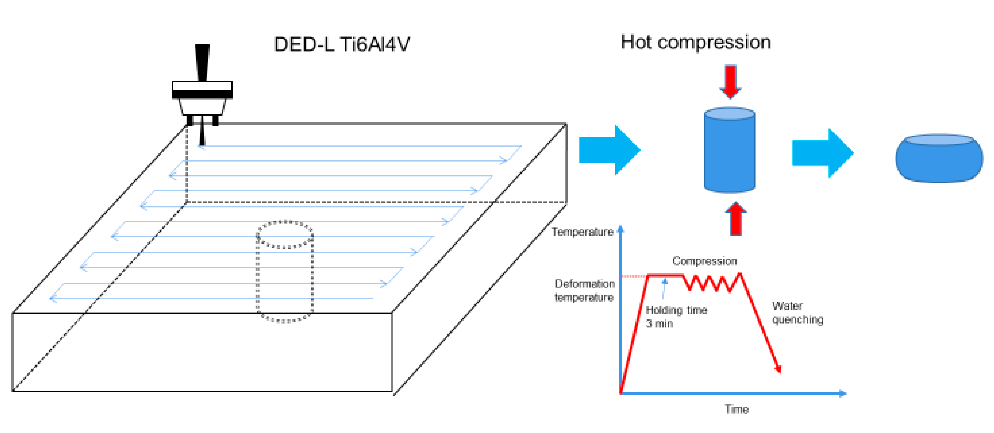
φ8 × 12 mm samples were cut off from the specimen. Isothermal compression test was carried out on Gleeble-3800 thermal simulator (Dynamic Systems Inc, New York, NY, USA). The sample was heated at heating rate of 5 °C/s, held at the deformation temperature for 3 min and then reduced to 50% of the original height. The deformation temperature is 700 °C, 750 °C, 800 °C, 850 °C and 900 °C. The strain rate is 0.001 s−1, 0.01 s−1, 0.1 s−1 and 1 s−1. The diagrammatic sketch of the experimental procedure is shown in Figure 2. The flow stress and strain values were measured by formula ε = l n ( ( l Δ l ) / l ) , σ = ( F ( l Δ l ) ) / ( A r e a l ) , where l is the original height of the sample, Δl is the reduction, A r e a is the original section area of the circular section of the cylinder, F   is force. The constant strain rate loading is obtained by controlling the increase of Δl with time. The flow stress curves were corrected for the effect of adiabatic temperature rise [20]. Graphite flakes were added between the end face of sample and anvil to reduce friction. The softening effect caused by thermal effect during deformation can be calculated by formula σ = Q n α R [ 1 T 1 T + Δ T ] , where Q is an activation energy, R is the gas constant (8.314 J/(mol·K), ΔT is measured by thermocouple, and n, α are material parameters, which are later presented in Equation (7). There is one sample for each experimental condition, and only one sample is added when the experimental results are obviously abnormal.

3. Results and Discussion

3.1. Flow Behavior

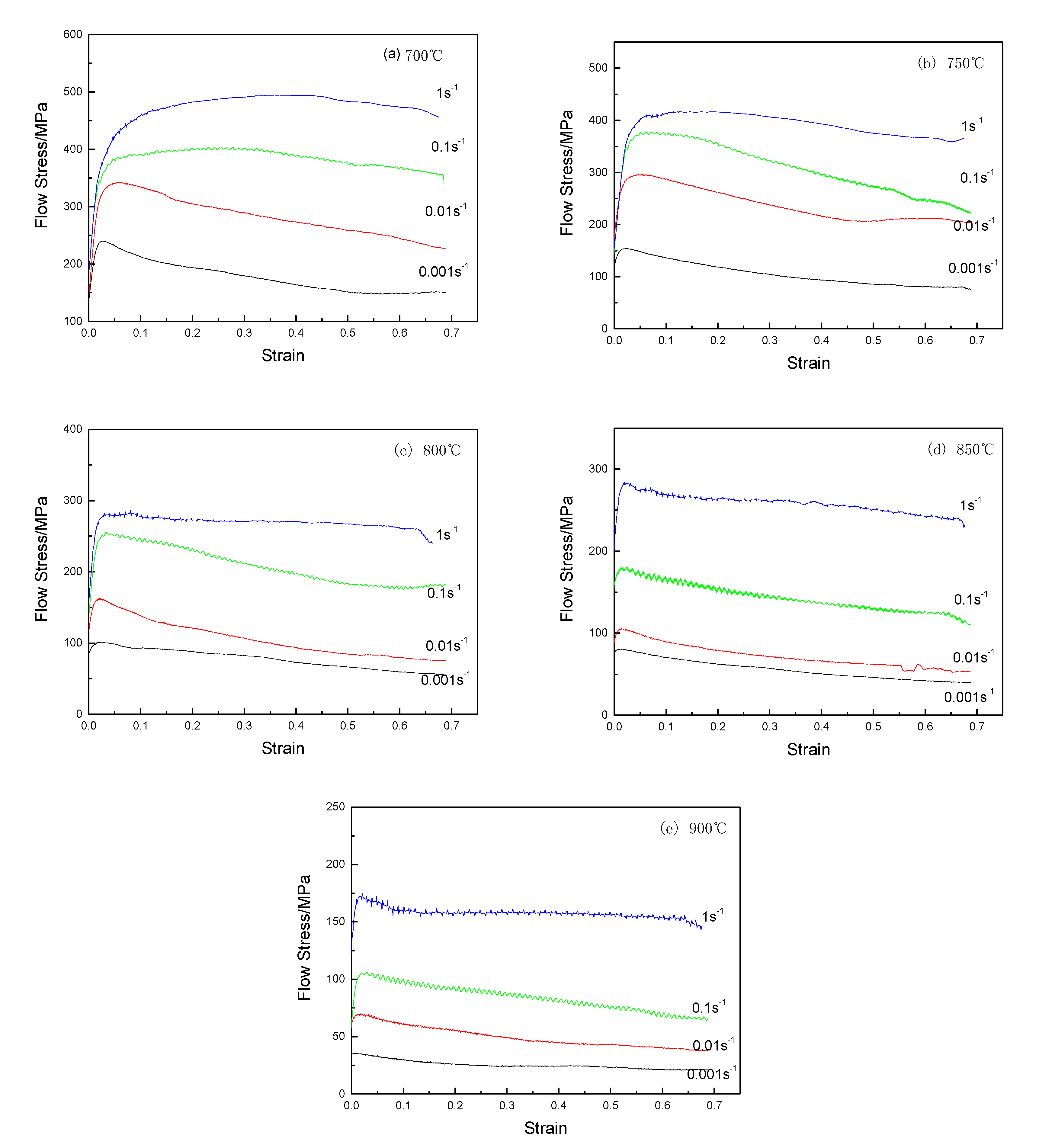
Flow stress–strain curves of DEDL Ti6Al4V alloy are shown in Figure 3. Obviously, the flow stress decreases with the increase of deformation temperature and the decrease of strain rate. The material show dynamic recrystallization at all strain rate, where the flow stress first increases to peak value, and then gradually decrease to a near steady state. This type of flow stress–strain curves are typically obtained in hot deformation of Ti6Al4V alloy with transformed β microstructure [21]. The shape of flow stress–strain curve is different at different deformation temperature and strain rate, which makes it more difficult to establish the constitutive relation accurately.

3.2. Modified Johnson–Cook Model

Johnson and Cook put forward Johnson–Cook model for the first time in 1983 [14]. Because of its simple form, it has been widely used soon after it was proposed. The model is expressed as
σ = ( A + B ε n ) ( 1 + C l n ε ˙ * ) ( 1 + T * m )
ε ˙ * = ε ˙ / ε ˙ r e f
T * m = ( T T r e f ) ( T m T r e f )
where σ is the flow stress, ε is the strain, ε ˙   is strain rate, ε ˙ r e f is reference strain rate, T is the deformation temperature, Tm is the melting temperature, Tref is the reference temperature, and A, B, n, and C are four materials constants. However, the original J-C model assumed that temperature, strain rate and strain had independent influences on flow stress. Lin et al. [22] considered the influence of strain position and the coupling influence of temperature and strain rate on the flow behavior of 43 CrMo alloy, and proposed an modified J-C model, as shown in Equation (4). This model has been used to predict the flow stress of titanium alloys [23].
σ = ( A 1 + B 1 ε + B 2 ε 2 ) ( 1 + C 1 ln ε ˙ * ) exp [ ( λ 1 + λ 2 ln ε ˙ * ) ( T T r e f ) ]
where A1, B1, B2, C1, λ1, and λ2 are the materials constants, the meaning of other symbols is the same as in original J-C model. The six materials constants can be computed using the traditional linear regression method (TLRM) in [22].
Take Tref = 700 °C and ε ˙ r e f = 1   s 1 to determine the constants in Equation (4). Substitute flow stress and strain at 700 °C and 1 s−1 to Equation (4), and conduct two-order polynomial fitting, as shown in Figure 4. A 1 , B 1 , and B 2 , were calculated to be 433.37 MPa, 319.22 MPa, and −427.97 MPa respectively.
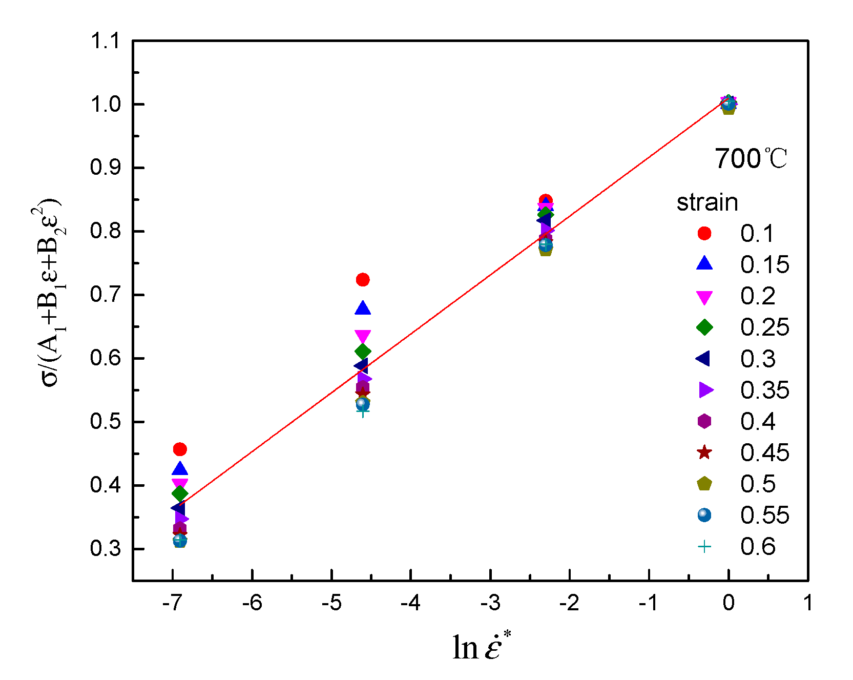
Substitute flow stress and strain at 700 °C and different strain rate, then plot σ / ( A 1 + B 1 ε + B 2 ε 2 ) vs. l n ε ˙ * , and conduct liner fitting, as shown in Figure 5. The value of C 1 was determined to be 0.09276.
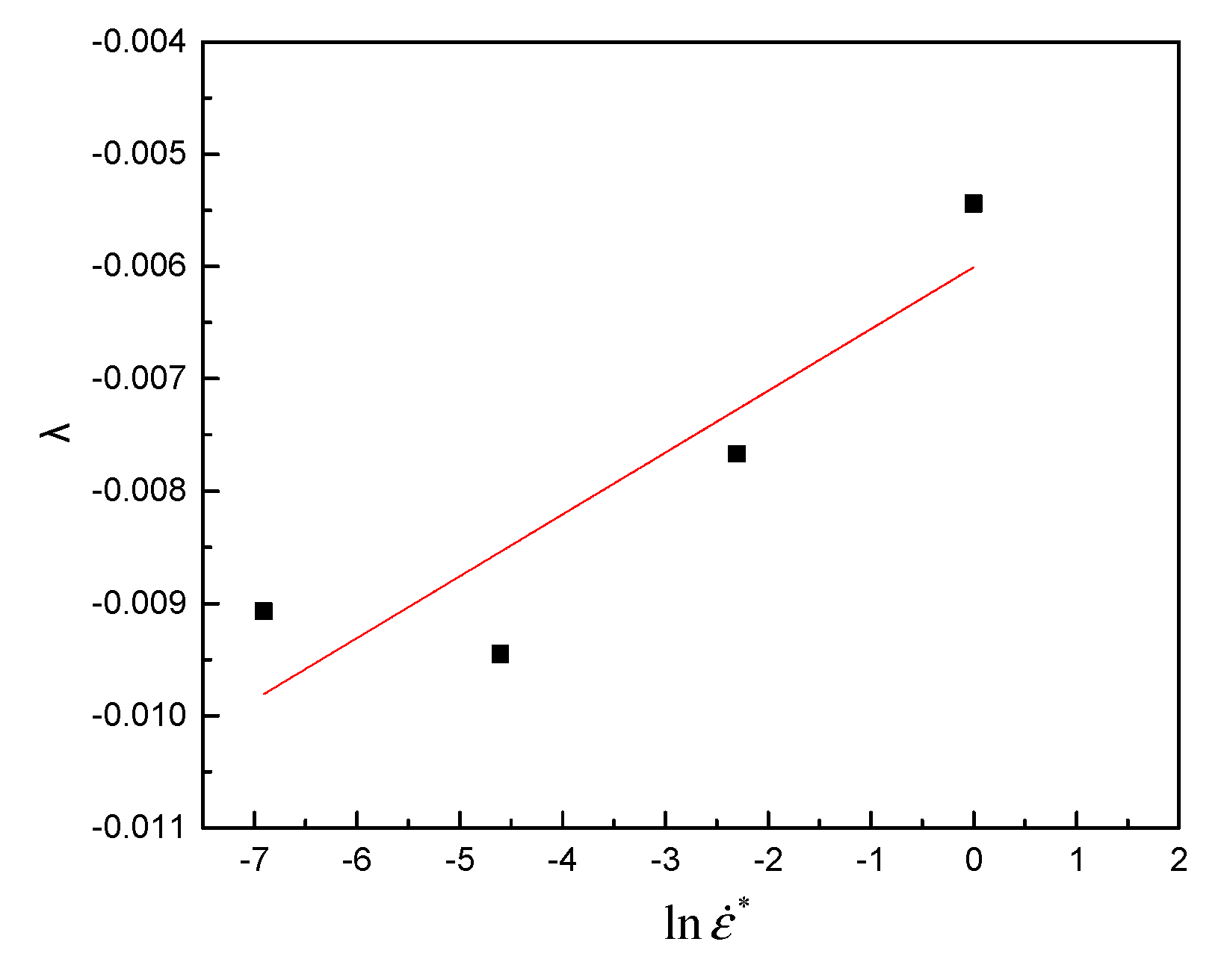
Introducing a new parameter λ = λ 1 + λ 2 ln ε ˙ * , the relationship between ln ( σ / ( A 1 + B 1 ε + B 2 ε 2 ) ( 1 + C 1 ln ε ˙ * ) ) and T T r e f at different strain rate was obtained as shown in Figure 6, and λ = λ 1 + λ 2 l n ε ˙ * values for strain rate of 1 s−1, 0.1 s−1, 0.01 s−1, and 0.001 s−1 were determined to be −0.00544, −0.00767, −0.00945, and −0.00907 respectively. From the plot of λ vs. l n ε ˙ * , λ 1 , and λ 2 were computed as −0.00601 and 0.0005502 respectively.
The six constants in Equation (4) can also be directly fitted by IBM SPSS Statistics software (version 19, IBM, Chicago, IL, USA) with a nonlinear regression analysis (NRA), as shown in Table 2. The optimal goal of NRA is to minimize the residual sum of squares between predicted and tested values. The method of NRA fitting is simple and fast. The influence of this method on the accuracy of modified J-C model is also evaluated.
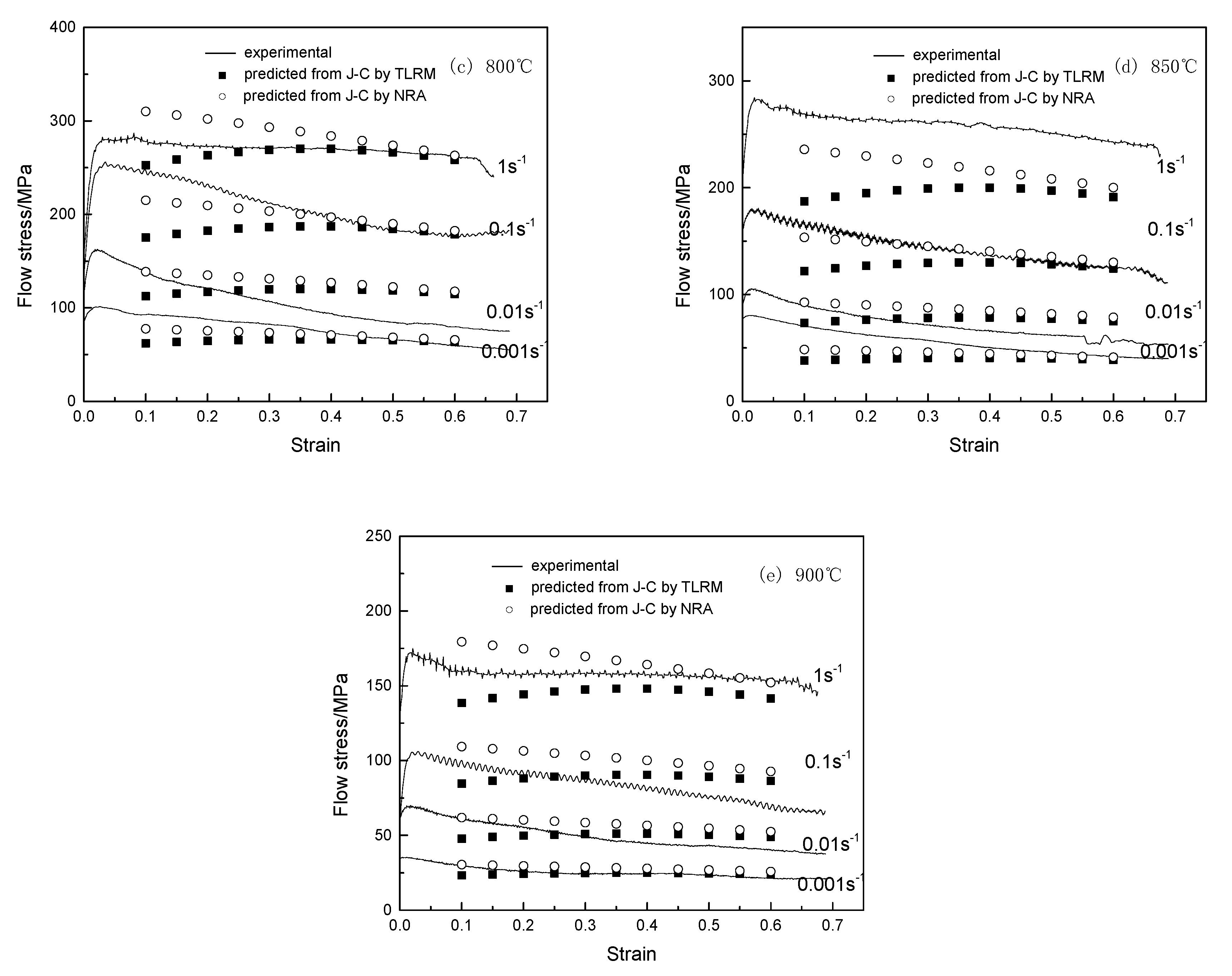
Figure 7 shows the experimental and predicted flow stress–strain curves from modified J-C model by TLRM and NRA. The predicted and experimental values show large deviation at strain less than 0.4. By comparing the results of TLRM and NRA, it can be concluded that NRA can improve the accuracy of modified J-C model at strain lower than 0.4. When the strain is greater than 0.4, the prediction results of the two methods are similar. The quantitative impact is discussed in Section 3.5.

3.3. Strain Compensated Arrhenius Model (SCAM)

The relationship between flow stress, strain rate and temperature can be expressed by the Arrhenius constitutive equation [15]
Z = ε ˙ exp ( Q / R T ) = A 2 σ n 1 ( α σ < 0.8 )
Z = ε ˙ exp ( Q / R T ) = A 3 [ exp ( β σ ) ] ( α σ > 1.2 )
Z = ε ˙ exp ( Q / R T ) = A 4 [ sinh ( α σ ) ] n 2   for   all   stress
where ε ˙ is the strain rate; σ is the flow stress; T is absolute temperature; Z is the temperature-compensated strain rate; Q is an activation energy; R is the gas constant (8.314 J/(mol·K); A 2 , A 3 , A 4 , n 1 n 2 , β , and α are material parameters. Equation (7) can be simplified to Equation (5) At low stress level (i.e., α σ < 0.8 ), and can be simplified to Equation (6) At high stress levels (i.e., α σ > 1.2 ). The material constant α was an adjustable parameter to produce parallel lines in a plot of ln [ s i n h ( α σ ) ] vs. l n ε ˙ [24]. These four materials constants in Equation (7) at a fix strain can be calculated by traditional linear regression method (TLRM), artificial neural network [25], and other methods [26].
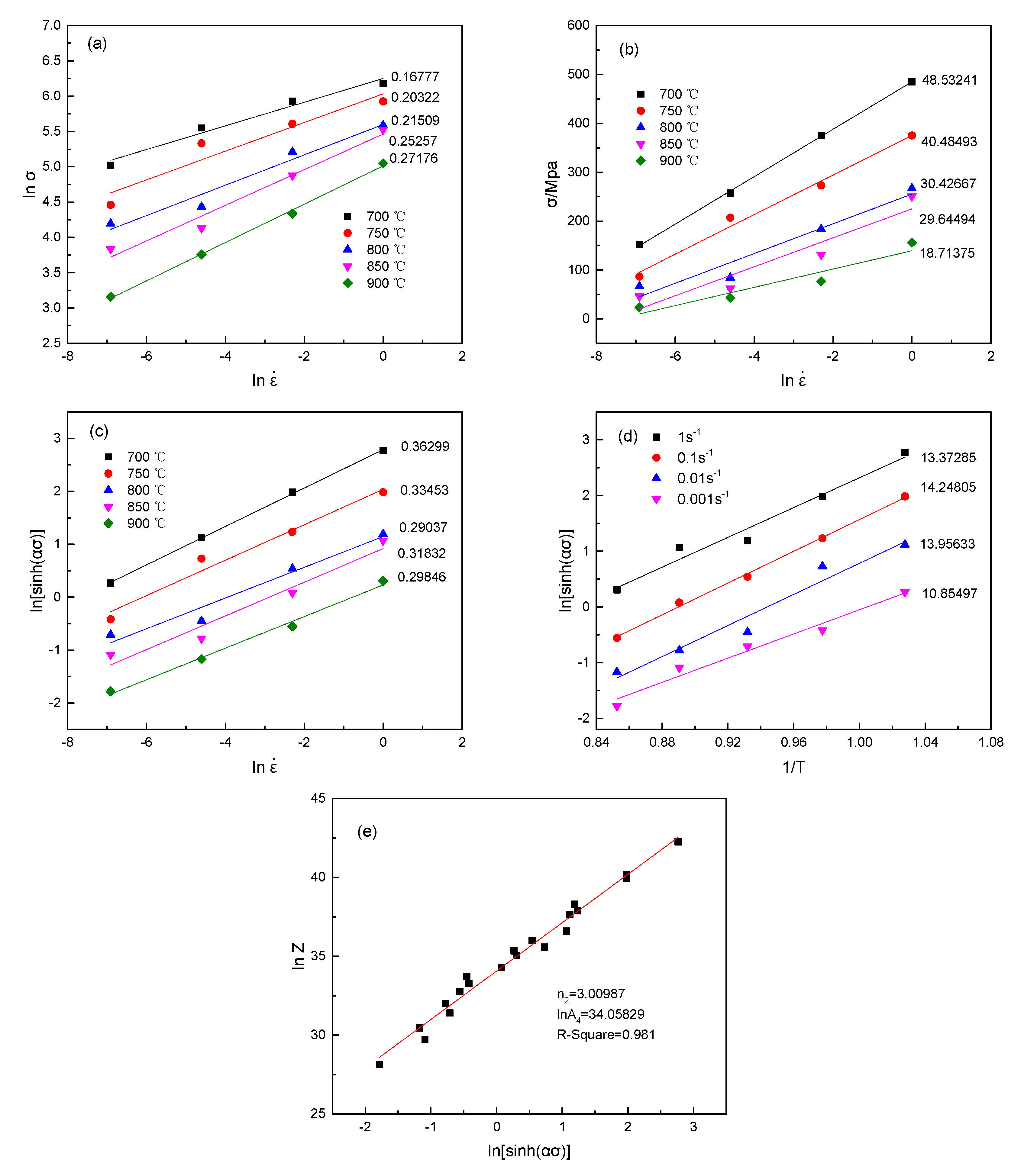
Taking the strain of 0.5 as an example, the TLRM to determine the material constants under fixed strain are illustrated [27]. The values of n 1 and β can be obtained from the mean slope values of ln σ - l n ε   ˙ and σ - l n ε   ˙ plots, as shown in Figure 8a,b. Then, α can be calculated using α = β / n 1 . The Q value can be determined by calculating the slopes of ln [ s i n h ( α σ ) ] l n ε   ˙ and ln [ s i n h ( α σ ) ] 1 / T plots respectively shown in Figure 8c,d. The ln A 4 and n 2 values can be determined by calculating the intercept and slope of ln [ s i n h ( α σ ) ] ln Z plot shown in Figure 8e.
The four constants in Equation (7) at a fixed strain can also be fitted by IBM SPSS Statistics software (version 19, IBM, Chicago, IL, USA) with a nonlinear regression analysis (NRA).
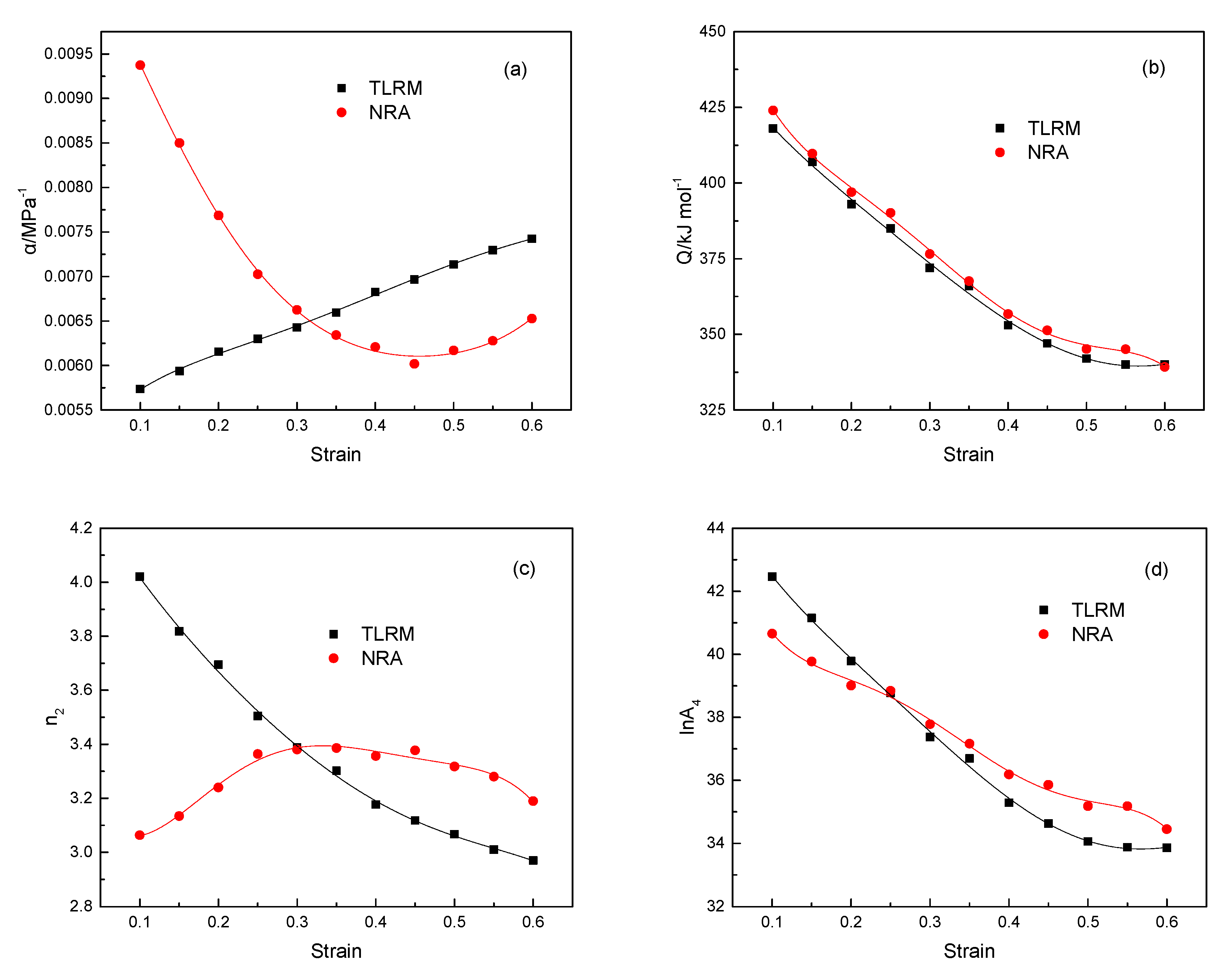
The material constants at strain range of 0.1–0.6 at the interval of 0.05 were calculated by TLRM and NRA respectively, as shown in Figure 9. The material constant α was an adjustable parameter to produce parallel lines in a plot of ln [ sin h ( α σ ) ] vs. l n ε   ˙ [24], and has great influence on the prediction accuracy of the model. This parameter can be determined by TLRM, or by trial and error to obtain the minimum slope deviation, or other methods. The value of α obtained by TLRM is comparable to that of TC4, TC17, and has the same change rule with the increase of strain. Compared with TLRM, NRA has a great influence on α and n 2 and their variation law with strain. At the same time, it has little influence on Q and l n A 4 and their variation law with strain. In fact, constant α at strain of 0.5 calculated by TLRM was 0.0073, and the slope values are 0.36299, 0.33453, 0.29037, 0.31832, and 0.29846, shown in Figure 8c. The constant α calculated by NRA was 0.00617, the slope values are 0.32229, 0.30542, 0.27273, 0.30277, and 0.2919. The corresponding standard deviations are 0.0292 and 0.0183 respectively. Therefore, more parallel lines are obtained by using the NRA method in a plot of ln [ sin h ( α σ ) ] vs.   l n ε   ˙ . The Q value decrease from about 435 kJ·mol−1 to 340 kJ·mol−1 with strain increasing from 0.1 to 0.6. These values are lower than that reported for conventional Ti6Al4V alloy [28,29]. Deformation activation energy can be used to characterize the degree of deformation difficulty. Since the deformation activation energy of DEDL Ti6Al4V is lower than that of traditional Ti6Al4V alloy, it can be concluded that DEDL is easier to deform.
The effect of strain is incorporated by assuming that four material constants in Equation (7) are polynomial function of strain [30]. These values are fitted by a fifth-order polynomial, and the coefficients of polynomial functions are given in Table 3 and Table 4.
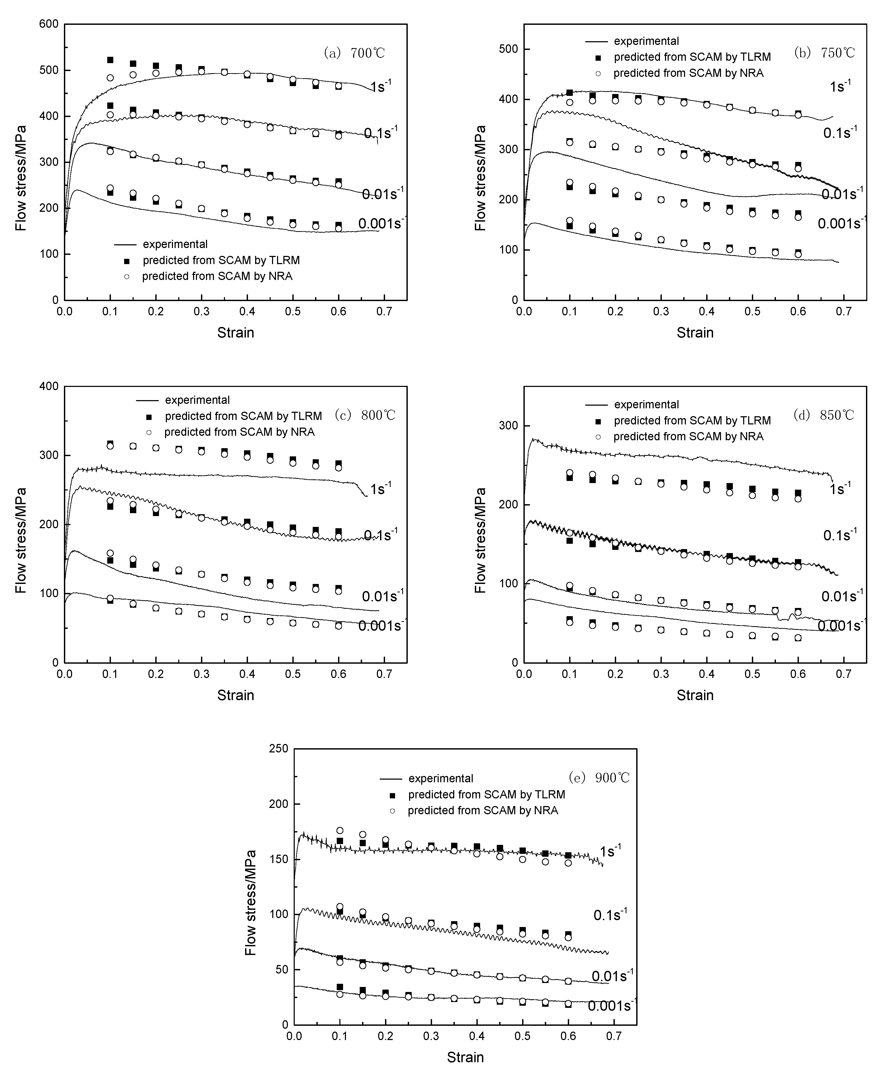
Figure 10 Shows the experimental and predicted flow stress–strain curves from SCAM by TLRM and NRA. As can be seen from Figure 10, the SCAM model accurately predicted flow stress; the prediction results of the two methods are similar. Further quantitative analysis will be carried out in Section 3.5.

3.4. Modified Fields–Backofen (F-B) Model

Fields and Bachofen [16] proposed the following common formula to describe the stress–strain relationship
σ = K ε n 3 ε ˙ m
X.H. Zhang [31] introduced the softening factor into F-B model to describe the softening behaviors for magnesium alloy. This modified equation can be expressed as
σ = K ε n 3 ε ˙ m exp ( b T + s ε )
The study on the flow stress of magnesium alloy AZ31 [32] and AZ61 [33] at high temperature shows that the material constants K, n 3 , and m can be can be assumed as
K = K 1 + K 2 l n ε ˙ + K 3 / T
n 3 = n 4 + n 5 ln ε ˙ + n 6 / T
m = m 1 + m 2 T
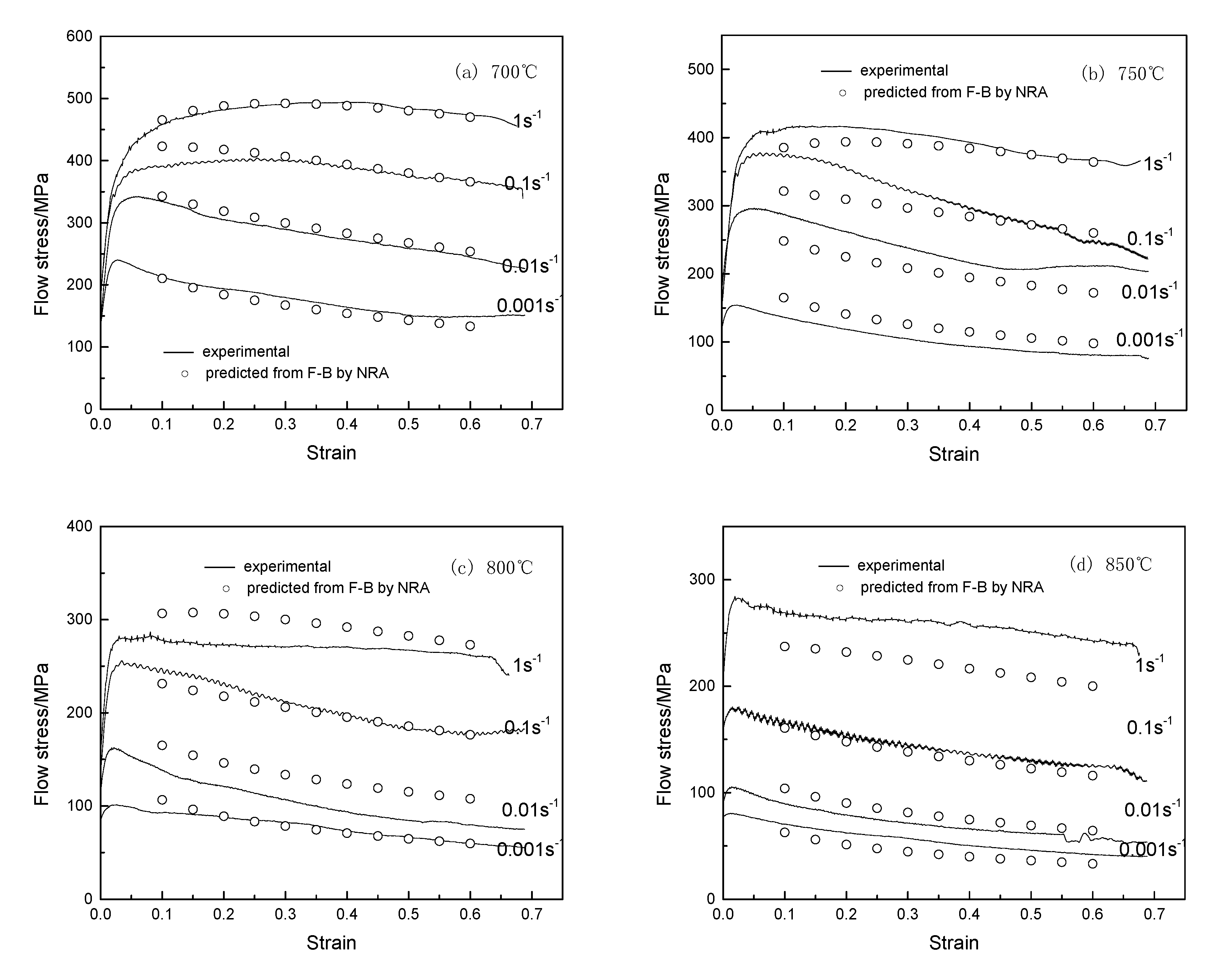
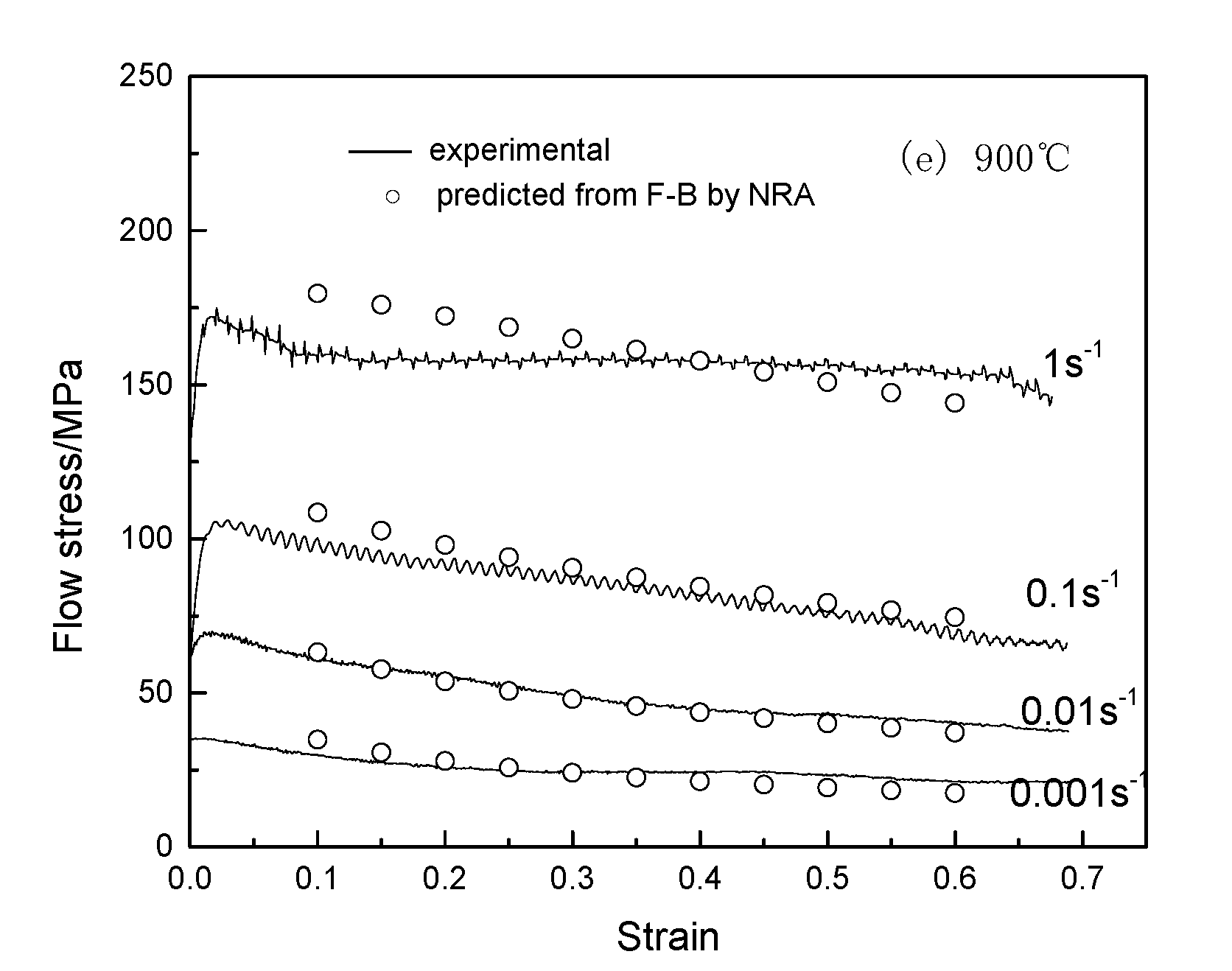
The 10 constants in Equations (9)–(12) were fitted by NRA and shown in Table 5. Figure 11 shows the experimental and predicted flow stress–strain curves from F-B model by NRA. It is shown that the modified F-B model can predict the flow stress well. In order to fit the experimental data more accurately, a more detailed form of parameters K and s are adopted for M50NiL steel [25]. Jia et al. introduce another softening factor exp ( C 0 / T ) , presume the parameters in Equation (8) as a polynomial function of strain, and describe the flow stress of as cast AZ31B alloy [34].

3.5. Evaluation of the Phenomenological Models

The accuracy of the phenomenological models is further quantitatively evaluated by standard statistical parameters, including correlation coefficient (R), average absolute relative error (AARE), and average root mean square error (RMSE). They can be expressed as:
R = i = 1 N ( E i E - ) ( P i P - ) i = 1 N ( E i E - ) 2 i = 1 N ( P i P - ) 2
A A R E ( % ) = 1 N i = 1 N | E i P i E i | × 100 %
R M S E = 1 N i = 1 N ( E i P i ) 2
where Ei is the experimental value, Pi is the predicted value, E ¯ and P ¯ are the mean value of NRAexperimental and predicted values, N is the total number.
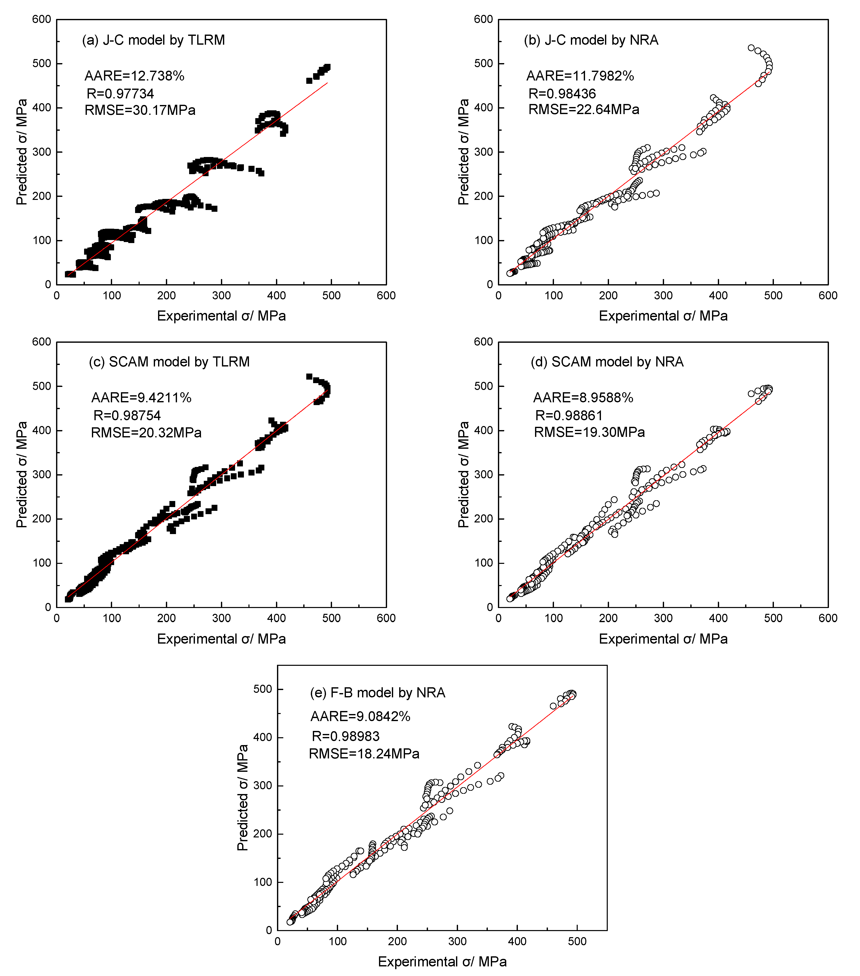
The calculated values of R, AARE, and RMSE are presented in Figure 12. The R values for modified J-C model by TLRM and NRA were 0.977 and 0.984, respectively. The corresponding AARE values were 12.74% and 11.80%, respectively, and the RMSE values were 30.17 MPa and 22.64 MPa. Through comparison, it is concluded that NRA can improve the accuracy of modified J-C model. When TLRM is used, the determination of parameters A1, B1, and B2 only takes into account the variation law of flow stress with strain under the conditions of reference temperature and strain rate. In the case of NRA, the parameters are determined by taking the residual sum of squares as the goal of fitting under all test conditions. Therefore, without considering the physical significance of specific parameters, the adoption of NRA for parameter determination can improve the prediction accuracy of the modified J-C model. Ning et al. [35,36] recently provided an effective and convenient determination method for J-C constants of metal materials in machining. The prediction accuracy can be improved by modifying the model or improving the parameter identification method.
The R values for SCAM model by TLRM and NRA were 0.987 and 0.989, respectively. The corresponding AARE values were 9.42% and 8.96%, respectively, and the RMSE values were 20.32 MPa and 19.3 MPa. It is concluded that NRA has limited effect on that of the accuracy SCAM model. This is because each of the test data was also used when TLRM and NRA were used to solve the four parameters in Equation (7). Therefore, the NRA had less influence on the SCAM results than it did on the J-C model.
The R values for modified J-C, SCAM and modified F-B models by NRA were 0.984, 0.986, and 0.99, respectively. The corresponding AARE values were 11.8%, 8.96%, and 9.08%, respectively, and the RMSE values were 22.64 MPa, 19.3 MPa, and 18.24 MPa. It is indicated that the accuracy of modified F-B and SCAM model is higher than that of modified J-C model. In this study, there are 6, 10, and 24 material parameters in the modified J-C, F-B, and SCAM model, respectively. Among the three models in this study, the modified J-C model requires the minimum number of material parameters. In order to improve the accuracy of the modified J-C model, more complex material parameter expressions may be needed [37], or material parameters may be determined in different test intervals [38]. Recently, other expressions of strain effect were given by Niu et al. [39]. At the same time, strain rate hardening and temperature softening were expressed in more complex forms and were successfully applied to A356 alloy.

4. Conclusions

  • The deformation activation energy decrease from 435 kJ·mol−1 to 340 kJ·mol−1 with the increasing of strain increasing from 0.1 to 0.6, and this value is lower than that reported for conventional Ti6Al4V alloy.
  • The AARE values for modified J-C model by TLRM and NRA were 12.74% and 11.80%, and the corresponding RMSE values were 30.17 MPa and 22.64 MPa, respectively. The AARE values for modified SCAM model by TLRM and NRA were 9.42% and 8.96%, and the corresponding RMSE values were 20.32 MPa and 19.3 MPa, respectively. Compared with the TLRM, the NRA improves the accuracy of J-C model, while it has limited effect on that of SCAM model. Compared with traditional linear fitting, nonlinear fitting is more suitable for parameter identification of constitutive model.
  • The AARE values for modified J-C, SCAM, and modified F-B models by NRA were 11.8%, 8.96%, and 9.08%, respectively, and the corresponding RMSE values were 22.64 MPa, 19.3 MPa, and 18.24 MPa. The accuracy of modified F-B and SCAM model is higher than that of modified J-C model. The modified F-B model is most suitable for the flow stress prediction in this study.

Author Contributions

Y.N., literature search, figures, study design, data interpretation, writing; Z.S., study design, data analysis; Y.W., study design, data analysis; J.N., data collection. All authors have read and agreed to the published version of the manuscript.

Funding

This work was funded by the National Natural Science Foundation of China (grant no. 51875274), Taiyuan University of Science and Technology Science Research Initial Founding (grant no. 20192007), and Technological Innovation Programs of Higher Education Institutions in Shanxi (grant no. 2020L0351).

Acknowledgments

This work was supported by the National Natural Science Foundation of China (grant no. 51875274), Taiyuan University of Science and Technology Science Research Initial Founding (grant no. 20192007), and Technological Innovation Programs of Higher Education Institutions in Shanxi (grant no. 2020L0351).

Conflicts of Interest

The authors declare no conflict of interest.

References

  1. Liu, S.; Shin, Y.C. Additive manufacturing of Ti6Al4V alloy: A review. Mater. Des. 2019, 164, 107552. [Google Scholar] [CrossRef]
  2. Bambach, M.; Sizova, I.; Emdadi, A. Development of a processing route for Ti-6Al-4V forgings based on preforms made by selective laser melting. J. Manuf. Process. 2019, 37, 150–158. [Google Scholar] [CrossRef]
  3. Xie, Y.; Zhang, H.; Zhou, F. Improvement in geometrical accuracy and mechanical property for arc-based additive manufacturing using metamorphic rolling mechanism. J. Manuf. Sci. Eng. 2016, 138, 111002. [Google Scholar] [CrossRef]
  4. Colegrove, P.A.; Coules, H.E.; Fairman, J.; Martina, F.; Kashoob, T.; Mamash, H.; Cozzolino, L.D. Microstructure and residual stress improvement in wire and arc additively manufactured parts through high-pressure rolling. J. Mater. Process. Technol. 2013, 213, 1782–1791. [Google Scholar] [CrossRef]
  5. Donoghue, J.; Antonysamy, A.A.; Martina, F.; Colegrove, P.A.; Williams, S.W.; Prangnell, P.B. The effectiveness of combining rolling deformation with Wire–Arc Additive Manufacture on β-grain refinement and texture modification in Ti–6Al–4V. Mater. Charact. 2016, 114, 103–114. [Google Scholar] [CrossRef]
  6. Zhao, Y.; Sun, J.; Li, J.; Yan, Y.; Wang, P. A comparative study on Johnson-Cook and modified Johnson-Cook constitutive material model to predict the dynamic behavior laser additive manufacturing FeCr alloy. J. Alloy. Compd. 2017, 723, 179–187. [Google Scholar] [CrossRef]
  7. Bambach, M.; Sizova, I.; Silze, F.; Schnick, M. Hot workability and microstructure evolution of the nickel-based superalloy Inconel 718 produced by laser metal deposition. J. Alloy. Compd. 2018, 740, 278–287. [Google Scholar] [CrossRef]
  8. Bambach, M.; Sizova, I.; Szyndler, J.; Bennett, J.; Hyatt, G.; Cao, J.; Papke, T.; Merklein, M. On the hot deformation behavior of Ti-6Al-4V made by additive manufacturing. J. Mater. Process. Technol. 2021, 288, 116840. [Google Scholar] [CrossRef]
  9. Saboori, A.; Abdi, A.; Fatemi, S.A.; Marchese, G.; Biamino, S.; Mirzadeh, H. Hot deformation behavior and flow stress modeling of Ti–6Al–4V alloy produced via electron beam melting additive manufacturing technology in single β-phase field. Mater. Sci. Eng. A 2020, 792, 139822. [Google Scholar] [CrossRef]
  10. Rahmaan, T.; Abedini, A.; Butcher, C.; Pathak, N.; Worswick, M.J. Investigation into the shear stress, localization and fracture behaviour of DP600 and AA5182-O sheet metal alloys under elevated strain rates. Int. J. Impact Eng. 2017, 108, 303–321. [Google Scholar] [CrossRef]
  11. Abedini, A.; Noder, J.; Kohar, C.P.; Butcher, C. Accounting for Shear Anisotropy and Material Frame Rotation on the Constitutive Characterization of Automotive Alloys using Simple Shear Tests. Mech. Mater. 2020, 148, 103419. [Google Scholar] [CrossRef]
  12. Martina, F.; Colegrove, P.A.; Williams, S.W.; Meyer, J. Microstructure of Interpass Rolled Wire + Arc Additive Manufacturing Ti-6Al-4V Components. Metall. Mater. Trans. 2015, 46, 6103–6118. [Google Scholar] [CrossRef] [Green Version]
  13. Lin, Y.C.; Chen, X.M. A critical review of experimental results and constitutive descriptions for metals and alloys in hot working. Mater. Des. 2011, 32, 1733–1759. [Google Scholar] [CrossRef]
  14. Johnson, G.; Cook, W.H.C. A constitutive model and data for metals subjected to large strains, high strain rates and high temperatures. In Proceedings of the Seventh International Symposium on Ballistics, Den Haag, The Netherlands, 19–21 April 1983; pp. 541–547. [Google Scholar]
  15. Sellars, C.; Tegart, W.M. Hot workability. Int. Metall. Rev. 1972, 17, 1–24. [Google Scholar] [CrossRef]
  16. Fields, D.S.; Backofen, W.A. Determination of strain hardening characteristics by torsion testing. Proc. Am. Soc. Test. Mater 1957, 57, 1259–1272. [Google Scholar]
  17. Shen, J.; Hu, L.; Sun, Y.; Wan, Z.; Feng, X.; Ning, Y. A Comparative Study on Artificial Neural Network, Phenomenological-Based Constitutive and Modified Fields–Backofen Models to Predict Flow Stress in Ti-4Al-3V-2Mo-2Fe Alloy. J. Mater. Eng. Perform. 2019, 28, 4302–4315. [Google Scholar] [CrossRef]
  18. Kotkunde, N.; Deole, A.D.; Gupta, A.K.; Singh, S.K. Comparative study of constitutive modeling for Ti–6Al–4V alloy at low strain rates and elevated temperatures. Mater. Des. 2014, 55, 999–1005. [Google Scholar] [CrossRef]
  19. Ji, S.; Sun, Z.; Zhang, W.; Chen, X.; Xie, G.; Chang, H. Microstructural evolution and high temperature resistance of functionally graded material Ti-6Al-4V/Inconel 718 coated by directed energy deposition-laser. J. Alloy. Compd. 2020, 848, 156255. [Google Scholar] [CrossRef]
  20. Devadas, C.; Baragar, D.; Ruddle, G.; Samarasekera, I.V.; Hawbolt, E.B. The thermal and metallurgical state of steel strip during hot rolling: Part II. Factors influencing rolling loads. Metall. Mater. Trans. A 1991, 22, 321–333. [Google Scholar] [CrossRef]
  21. Seshacharyulu, T.; Medeiros, S.C.; Morgan, J.T.; Malas, J.C.; Frazier, W.G.; Prasad, Y.V.R.K. Hot deformation and microstructural damage mechanisms in extra-low interstitial (ELI) grade Ti–6Al–4V. Mater. Sci. Eng. A 2000, 279, 289–299. [Google Scholar] [CrossRef]
  22. Lin, Y.C.; Chen, X.-M.; Liu, G. A modified Johnson–Cook model for tensile behaviors of typical high-strength alloy steel. Mater. Sci. Eng. A 2010, 527, 6980–6986. [Google Scholar] [CrossRef]
  23. Cai, J.; Wang, K.; Zhai, P.; Li, F.; Yang, J. A Modified Johnson-Cook Constitutive Equation to Predict Hot Deformation Behavior of Ti-6Al-4V Alloy. J. Mater. Eng. Perform. 2015, 24, 32–44. [Google Scholar] [CrossRef]
  24. Slooff, F.A.; Zhou, J.; Duszczyk, J.; Katgerman, L. Constitutive analysis of wrought magnesium alloy Mg–Al4–Zn1. Scr. Mater. 2007, 57, 759–762. [Google Scholar] [CrossRef]
  25. Ji, G.; Li, L.; Qin, F.; Zhu, L.; Li, Q. Comparative study of phenomenological constitutive equations for an as-rolled M50NiL steel during hot deformation. J. Alloy. Compd. 2017, 695, 2389–2399. [Google Scholar] [CrossRef]
  26. Wang, H.; Zhang, Z.; Zhai, R.; Ma, R.; Zhao, J. New Method to Develop High Temperature Constitutive Model of Metal Based on the Arrhenius-Type Model. Mater. Today Commun. 2020, 24, 101000. [Google Scholar] [CrossRef]
  27. Li, L.; Li, M. Constitutive model and optimal processing parameters of TC17 alloy with a transformed microstructure via kinetic analysis and processing maps. Mater. Sci. Eng. A 2017, 698, 302–312. [Google Scholar] [CrossRef]
  28. Luo, J.; Li, M.; Li, H.; Yu, W. Effect of the strain on the deformation behavior of isothermally compressed Ti–6Al–4V alloy. Mater. Ence Eng. A 2008, 505, 88–95. [Google Scholar] [CrossRef]
  29. Jha, J.S.; Toppo, S.P.; Singh, R.; Tewari, A.; Mishra, S.K. Flow stress constitutive relationship between lamellar and equiaxed microstructure during hot deformation of Ti6Al4V. J. Mater. Process. Technol. 2019, 270, 216–227. [Google Scholar] [CrossRef]
  30. Cai, J.; Li, F.; Liu, T.; Bo, C.; Min, H. Constitutive equations for elevated temperature flow stress of Ti–6Al–4V alloy considering the effect of strain. Mater. Des. 2011, 32, 1144–1151. [Google Scholar] [CrossRef]
  31. Zhang, X. Experimental and Numberical Study of Magnesium durging Hot Working Process. Ph.D. Thesis, Shanghai Jiaotong University, Shanghai, China, 2003. [Google Scholar]
  32. Cheng, Y.Q.; Zhang, H.; Chen, Z.H.; Xian, K.F. Flow stress equation of AZ31 magnesium alloy sheet during warm tensile deformation. J. Mater. Process. Technol. 2008, 208, 29–34. [Google Scholar] [CrossRef]
  33. Tsao, L.C.; Huang, Y.T.; Fan, K.H. Flow stress behavior of AZ61 magnesium alloy during hot compression deformation. Mater. Des. 2014, 53, 865–869. [Google Scholar] [CrossRef]
  34. Jia, W.; Xu, S.; Le, Q.; Fu, L.; Ma, L.; Tang, Y. Modified Fields-Backofen model for constitutive behavior of as-cast AZ31B magnesium alloy during hot deformation. Mater. Des. 2016, 106, 120–132. [Google Scholar] [CrossRef]
  35. Ning, J.; Liang, S.Y. Inverse identification of Johnson-Cook material constants based on modified chip formation model and iterative gradient search using temperature and force measurements. Int. J. Adv. Manuf. Technol. 2019, 102, 2865–2876. [Google Scholar] [CrossRef]
  36. Ning, J.; Nguyen, V.; Huang, Y.; Hartwig, K.T.; Liang, S.Y. Inverse determination of Johnson–Cook model constants of ultra-fine-grained titanium based on chip formation model and iterative gradient search. Int. J. Adv. Manuf. Technol. 2018, 99, 1131–1140. [Google Scholar] [CrossRef]
  37. Li, H.Y.; Wang, X.F.; Duan, J.Y.; Liu, J.J. A modified Johnson Cook model for elevated temperature flow behavior of T24 steel. Mater. Ence Eng. A 2013, 577, 138–146. [Google Scholar] [CrossRef]
  38. Wang, Y.; Zhang, C.; Yang, Y.; Wang, Y.; Chen, L. The identification of improved Johnson-Cook constitutive model in a wide range of temperature and its application in predicting FLCs of Al–Mg–Li sheet. J. Mater. Res. Technol. 2020, 9, 3782–3795. [Google Scholar] [CrossRef]
  39. Niu, L.; Cao, M.; Liang, Z.; Han, B.; Zhang, Q. A modified Johnson-Cook model considering strain softening of A356 alloy. Mater. Ence Eng. A 2020, 789, 139612. [Google Scholar] [CrossRef]
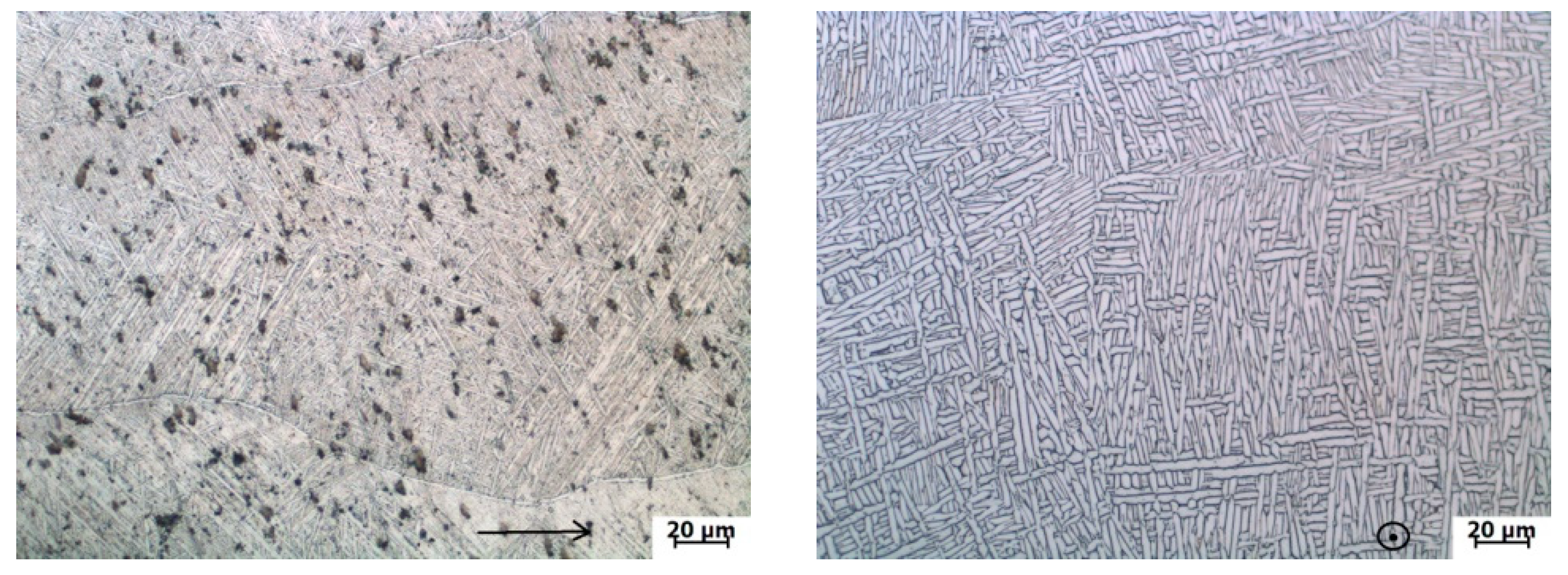
Figure 1. Optical microscopy micrograph of the DEDL (directed energy deposition laser) Ti6Al4V.
Metals 10 01496 g001
Figure 2. Diagrammatic sketch of the experimental procedure.
Metals 10 01496 g002
Figure 3. Flow stress–strain curves of DEDL Ti6Al4V alloy: (a) 700 °C, (b) 750 °C, (c) 800 °C, (d) 850 °C, (e) 900 °C.
Metals 10 01496 g003
Figure 4. Plot of σ vs. ε at 700 °C and 1 s−1.
Metals 10 01496 g004
Figure 5. Relationship between σ / ( A 1 + B 1 ε + B 2 ε 2 ) and l n ε ˙ * .
Metals 10 01496 g005
Figure 6. Relationship between   λ and l n ε ˙ * .
Metals 10 01496 g006
Figure 7. Experimental and predicted flow stress–strain curves from modified J-C model: (a) 700 °C, (b) 750 °C, (c) 800 °C, (d) 850 °C, (e) 900 °C.
Metals 10 01496 g007aMetals 10 01496 g007b
Figure 8. Plots of (a) ln ln σ -   l n ε   ˙ , (b) σ -   l n   ε   ˙ , (c) ln [ sin h ( α σ ) ] ln ε ˙ , (d) ln [ sin h ( α σ ) ] 1 / T and (e) ln [ sin h ( α σ ) ] ln Z at a strain of 0.5.
Metals 10 01496 g008
Figure 9. Materials constants calculated by TLRM and NRA: (a) α , (b) Q , (c) n 2 , and (d) l n A 4 .
Metals 10 01496 g009
Figure 10. Experimental and predicted flow stress–strain curves from SCAM model: (a) 700 °C, (b) 750 °C, (c) 800 °C, (d) 850 °C, (e) 900 °C.
Metals 10 01496 g010
Figure 11. Experimental and predicted flow stress–strain curves from modified F-B model: (a) 700 °C, (b) 750 °C, (c) 800 °C, (d) 850 °C, (e) 900 °C.
Metals 10 01496 g011aMetals 10 01496 g011b
Figure 12. Correlation between experimental and predicted flow stress from: (a) modified J-C by TLRM, (b) modified J-C by NRA, (c) SCAM by TLRM, (d) SCAM by NRA, and (e) modified F-B model by NRA.
Metals 10 01496 g012
Table 1. Chemical composition of Ti6Al4V powder.
ElementAlVCFeONHTi
Composition (wt %)6.0240.060.150.160.050.01Bal.
Table 2. Parameters for the modified J-C model.
ConstantsA1B1B2C1λ1λ2
TLRM433.37319.22−427.970.09276−0.006010.0005502
NRA548.83−122.17−58.0680.09143−0.005470.000561
Table 3. Polynomial fitting results of α , Q , n 2 , and ln A 4 by TLRM.
ParameterInterceptF1F2F3F4F5
α 0.004830.01377−0.06320.17456−0.221360.10374
Q 455.59−514.961945.3−6090.39009.3−4615.3
n 4.4958−5.794613.048−33.59456.381-35.985
ln A 46.977−64.879274.52−872.851304.2−687.92
Table 4. Polynomial fitting results of α , Q , n 2 , and ln A 4 by NRA.
ParameterInterceptF1F2F3F4F5
α 0.01114−0.01387−0.065990.34121−0.541740.30837
Q 504.66−1418.28552.8−28,36643,965−25,258
n 3.5120−12.246109.50−374.05563.21−316.30
ln A 48.139−143.28961.94−3229.24974.5−2844.5
Table 5. Parameters for the modified F-B model.
K1K2K3n4n5n6m1m2bs
10,772,259270,817.1−8,034,816,343−0.617450.037598−1.095160.00113−0.00846−0.46746733.0061
Publisher’s Note: MDPI stays neutral with regard to jurisdictional claims in published maps and institutional affiliations.