The Effect of Material Properties on the Accuracy of Superplastic Tensile Test


School of Applied Mathematics, National Research University Higher School of Economics, 123458 Tallinskaya 34, Moscow 123458, Russia
*
Author to whom correspondence should be addressed.
Metals 2020, 10(10), 1353; https://doi.org/10.3390/met10101353
Submission received: 27 August 2020
/
Revised: 1 October 2020
/
Accepted: 6 October 2020
/
Published: 10 October 2020
(This article belongs to the Special Issue Superplasticity and Superplastic Forming)
Abstract
:Tensile testing is widely used for the mechanical characterization of materials subjected to superplastic deformation. At the same time, it is known that the obtained flow data are affected by specimen geometry. Thus, they characterize the specimen rather than the material. This work provides the numerical analysis aimed to study how the material flow behavior affects the results of tensile tests. The simulations were performed by the finite element method in Abaqus software, utilizing user-defined procedures for calculation of forces acting on the crossheads. The accuracy of tensile testing is evaluated by the difference between the input material flow behavior specified in the simulations and the output one, obtained by the standard ASTM E2448 procedure based on the predicted forces. The results revealed that the accuracy of the superplastic tensile test is affected by the material properties. Even if the material flow behavior follows the Backofen power law, which is invariant for the effective strain, the output stress–strain curves demonstrate significant strain hardening and softening effects. The relation between the basic superplastic characteristics and the tensile test errors is described and analyzed.
1. Introduction
Superplastic sheet forming is a promising technology utilizing the ability of certain materials to reach extremely high deformations while forming at a specific temperature and strain-rate regimes [1,2]. The accurate mechanical characterization is critically important in the determination of such regimes and subsequent design of forming technologies. Thus, the experimental methods of mechanical testing, providing information about the flow behavior of superplastic materials, deserve extensive and thorough analysis. Aiming to reproduce the stress conditions realized in real forming processes, sustained efforts have been made to develop technological experiments and characterization techniques based on bulge [3,4,5,6], cone [7], and tube [8] forming tests. Nevertheless, tensile testing at constant strain rate remains the most widely used experimental way providing information about the deformation behavior of superplastic materials. Tensile testing is utilized for constitutive modeling of superplastic alloys [9,10,11,12,13], determination of optimal forming conditions, and the construction of material models for the design of forming technologies [14,15,16]. The stress–strain curves obtained by superplastic tensile tests at constant strain rates affect the microstructure changes during the deformation. Strain hardening at the lower strain rates is usually associated with grain growth; strain softening at higher strain rates is associated with dynamic recrystallization or void fraction growth [9].
Compared with the conventional tensile tests used for investigation of the stress–strain relations at room temperatures, the superplastic tensile test is a more complicated procedure. As the tests are performed at elevated temperatures, the use of extensometer or digital image correlation for deformation measurement is not feasible [17]. Thus, the strain rate is evaluated by the positions and velocities of the grips. At the same time, the viscoplastic character of deformation results in material flow from the grip area to the gauge region, which significantly affects the results, making them dependent on the specimen geometry. These aspects have been discussed in the literature in recent decades [18,19,20,21,22,23].
The effects of specimen geometry on the predicted deformation behavior of aluminum alloy 5083 at 550 °C, was studied by Khaleel et al. [18], providing both experimental and numerical studies of different specimen geometries with and without the alignment holes in the grips. They reported that the actual strain rate at the beginning of the test is about 60% of the desired one. Optimization of specimen geometry helped to reduce the deviation from the target strain rate to 10%. The effect of specimen geometry on the results of tensile tests of a similar alloy at 520 °C was analyzed experimentally and numerically by Sorgente and Tricarico [19]. Varying the specimen width and the fillet radius, they evaluated maximum measured stress and the elongation to failure. Numerical results were summarized using the indicators based on the differences between the strain and the strain rate in the center and the outer areas of a gauge section. The great importance of choosing the geometrical characteristics of a specimen was reported.
Various experimental trials and solutions improving the accuracy of the superplastic tensile test can be found in [20,21,22]. The gripping and specimen geometry issues, as well as heat and temperature effects, were discussed in [20]. Bate et al. [21] studied the effect of the gauge length on the results of the inhomogeneity of material flow during tensile testing. The final distribution of deformation throughout a specimen area was measured and analyzed. The stress–strain curves were corrected based on the evolution of the central cross-section area measured in the interrupted tests. An extensive experimental study, involving 24 different specimen geometries, was performed by Abu-Farha et al. [22]. The amount of material flow from the grip area to the gauge region was analyzed as the main source of errors in the superplastic tensile test. It was reported that the grip width to gauge width ratio, as well as the gauge length to gauge width ratio, should be equal to four in the optimized specimen geometry.
Compared to the pure experimental approach, the computer simulation of tensile tests gives a deeper understanding of the mechanical aspects of material flow and their role in the effects registered experimentally. Simulations can be used to predict the distributions of strain and strain rate within the specimen volume and study how these distributions are affected by the material properties or the specimen geometry. A comprehensive numerical investigation aimed to study the effect of specimen geometry in tensile testing of Ti6Al4V alloy at 900 °C was provided by Nazzal et al. [23]. The distribution of strain and strain rate within the specimen volume, as well as the material flow from the grip section to the gauge region, was studied for more than 30 specimen geometries. As a result, the recommendations to specimen geometry consistent with the ones provided in [22] are suggested.
The papers listed above highlight the important issues related to the superplastic tensile test. At the same time, since the investigations mentioned above were performed on a few specific alloys, they do not provide an understanding of how the material properties affect the effects described in them. Moreover, there is a lack of comprehensive analysis describing how accurately the stress–strain curves provided by the tensile testing reflect real material properties.
This work is aimed to provide a qualitative and quantitative analysis of the possible inaccuracies of superplastic tensile testing. As the geometry of a specimen affects the tensile test outcomes, the errors in the evaluation of stress–strain behavior are unavoidable. The effect of material properties on these errors is the particular focus of this study. Based on the results of finite element (FE) simulation of the tensile test procedure, the forces acting on the crossheads were calculated. Then, following the standard ATSM E2448 [17] procedure, the stress–strain curves were calculated as the output of the FE simulations. These output stress–strain curves were compared with the input ones corresponding to the actual material behavior assumed in the FE model. The deviations between these data were analyzed for different material properties.
2. Models and Methods
2.1. Finite Element Model
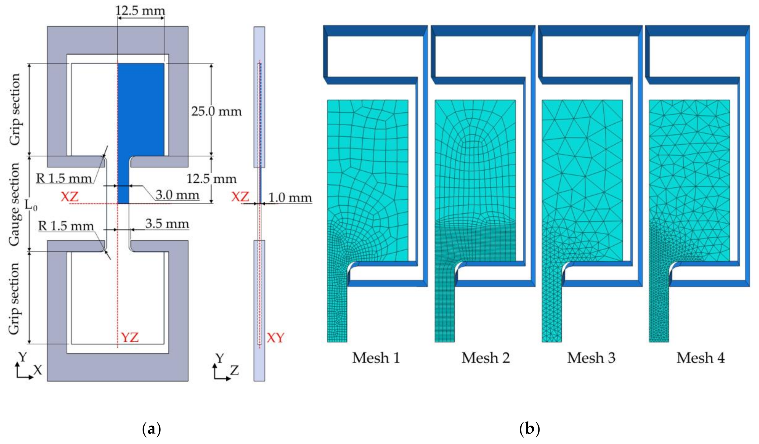
The tensile test procedure was simulated in SIMULIA Abaqus 2019 (Dassault Systèmes SE, Houston, TX, USA) using an “explicit/implicit” integration scheme. The reference geometrical model of a specimen was constructed according to the ASTM E2448 standard. Figure 1a presents the 1/8 part of a specimen used in the simulations with the symmetry boundary conditions at three faces corresponding to the orthogonal planes, which are denoted in the figure by the red dashed lines. Two types of FE mesh with different density were considered while examining the model accuracy. These FE meshes are presented in Figure 1b.
Based on the information provided in [23], the friction coefficient between the specimen and the grip shoulders was considered to be equal to 0.4. The grip was simulated as a rigid body, moving along the -axis with an increasing velocity ( to maintain the constant target strain rate (), as prescribed in the standard [17]:
where is the initial value of the gauge length and is the time of the process.
In the real experiments, the bottom crosshead remains unmoved, while the top one is moving with the velocity being twice as much as . As the process is very slow and all the dynamical effects are neglected, the material flow is symmetrical to the horizontal plane placed in the center of the specimen. As the material flow in the simulations was considered relative to this plane, the crosshead velocity was calculated according to the Equation (1).
2.2. The Constitutive Models
To study the effect of material properties on the results of tensile tests, different constitutive models describing the relation between stress, strain, and strain rate were implemented. As the mechanism-based and physically justified constitutive models require a large number of parameters, they are not feasible for the investigation of the role of material properties in the accuracy of tensile testing. This investigation requires the constitutive models with parameters, which clearly represent basic mechanical aspects of material flow as strain-rate sensitivity or strain hardening. Therefore, the phenomenological constitutive models generally applied in computer simulations of superplastic forming were utilized.
The basic behavior of superplastic materials is described by the Backofen equation:
where and are the material parameters. The strain-rate sensitivity () plays a major role in the process of superplastic deformation, as it is responsible for strain localization and necking [24]. Higher values of provide higher flow stability and larger tensile elongations. Superplastic materials have the value of , which is generally higher than 0.5 [25]. The values in the range of 0.3 to 0.5 provide a quasi-superplastic deformation [26]. For the materials with more complex deformation behavior than the one described by Equation (2), the value of strain-rate sensitivity is determined as a partial derivation of the stress with respect to the strain rate:
The Backofen model treats the material as an ideal viscous medium that does not demonstrate any deformation effects such as strain hardening or softening. The simplest model involving the strain hardening effect is based on the power law:
where is the material constant referred to as the strain hardening index and is the effective strain.
To study the effect of basic material properties (the strain-rate sensitivity and the strain hardening) on the accuracy of tensile testing, more than 30 simulations were performed with different parameters of the Equations (2) and (4). More complex material models were examined by the additional simulations using the specific sets of parameters presented below.
One of the important features of superplastic materials is the variation of the strain-rate sensitivity with the strain rate. As the Equations (2) and (4) do not take this variation into account, they are generally used as the local approximations of the material behavior. The variation of with the strain rate usually has a dome-like shape [27], thus the log stress vs. log strain rate relation appears like a sigmoidal function. One of the possible approximations of such deformation behavior is given by the following equation [28]:
where , , , and are treated as material constants.
In this work, Equation (5) was used to study the effect of strain rate on the results of tensile testing. The values of the material constants corresponding to the Ti6Al4V alloy at 875 °C [29] ( = 10.38 MPa, = 92.10 MPa, = 267.7, and = 1.33) were used in the simulations.
To study the effects of strain softening and variation of with the effective strain, the approximation of the experimental data presented in [30] was used. The constitutive model is given by the following equation:
where , , , , , , , , , and are the material parameters. The parameter set provided in [30] that corresponds to the AA5083 alloy at 470 °C was used in the simulations.
The deformation behavior of the specimen material was specified using the “creep” model in Abaqus software: , where is the effective stress, is referred to as the power-law multiplier, and —as the effective stress order.
The Equations (2), (4)–(6) describe the material behavior as a relation of the effective stress on the effective strain (ε) and the effective strain rate. To define such behavior in the model, the parameters and were treated as the functions of and specified in table form. To fill the table for corresponding strain and strain-rate ranges, first, the strain-rate sensitivity () was calculated by Equation (3) as a function of strain and strain rate, then, the values of and were determined as and .
2.3. Calculation of the Output Stress and Strain
While the input stress–strain relations were specified before the simulations by the equations listed in the previous section, the output ones were calculated based on the simulation results. At each simulation increment, the values of the output strain () and the output stress () were calculated as prescribed by the ASTM E2448 standard [17]:
where is the current gauge length determined as the distance between the grip shoulders, is the initial grip width (6 mm) and is the initial grip thickness (1 mm), and is the force acting on the crossheads.
Calculation of the force acting on the crosshead was performed after the simulations, utilizing postprocessing Python scripts. The forces were calculated using two different ways:
where is the component of stress tensor which corresponds to the vertical direction (the direction of tension), is the area of the specimen cross-section by the horizontal symmetry plane, and is the volume of the upper half of the specimen. The values of , (effective stress), and (effective strain rate), used in Equations (9) and (10), are available as the results of FE simulation at each time increment in each element.
Equation (9) represents the way for calculation of the vertical force, acting on the horizontal plane placed in the center of the specimen. Necessarily satisfying the mechanical equilibrium of the specimen, this force is equal to the one acting on the tool. Integral in Equation (10) represents the amount of mechanical power developed by internal stresses. This power is equal to the one developed by the external forces (). The postprocessing Python scripts were written to implement both described methods of force calculation. The difference between the values calculated with different formulas was used to evaluate the accuracy of the FE simulations.
3. Results
3.1. The Adjustment and Verification of the Model
To verify the implemented algorithms for the force determination, they were applied in preliminary simulations, which reproduce the conditions of uniform uniaxial tension. The model of a box with dimensions of the grip region of the 1/8 tensile specimen (3 mm × 12.5 mm × 0.5 mm) was implemented in the Abaqus software. The -symmetry (the symmetry about a horizontal plane) boundary conditions were specified at the top and the bottom edges of this box. These boundary conditions define vertical components of the velocities of the mesh points. The bottom symmetry plane was fixed, while the top one moved in the direction with the velocity determined by Equation (1). As the deformation of this box is uniform, the accuracy of the implemented algorithms can be verified by the similarity of the input and output stress–strain relations.
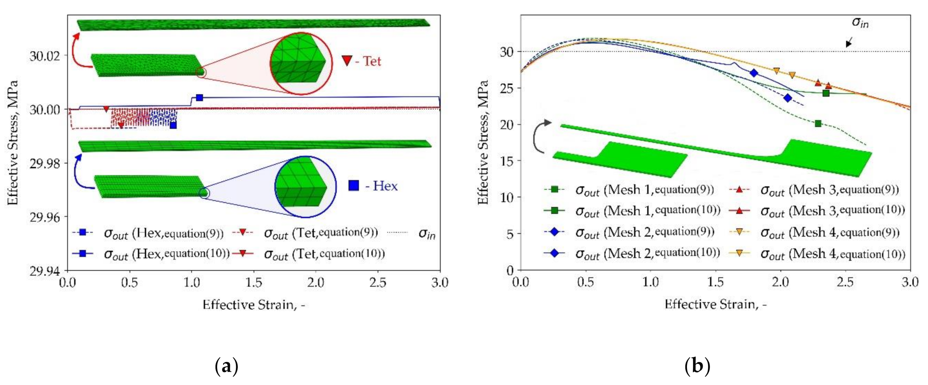
The results of the simulations for the Backofen material model, with parameters = 300 and = 0.5 and nominal strain rate , are presented in Figure 2. Figure 2a shows the output stress–strain curves obtained for box geometry using different meshes and different ways for force calculation. The same results obtained for the real tensile specimen geometry are presented in Figure 2b.
As the Backofen model does not involve any strain hardening/softening effects, the stress–strain curve for this model should appear as a straight horizontal line. As can be observed in Figure 2a, in the case of uniform uniaxial tension, the output stress deviates insignificantly from the value of 30 MPa corresponding to the input stress at . Both FE meshes demonstrate good accuracy in this case. The deviations from the input stress value are less than 0.01 MPa (0.03%). Different ways of force calculation provide very close outcomes. The first one results in slightly lower stresses, but the deviation is less than 0.01 MPa. This demonstrates that the force calculation algorithms were implemented correctly, both for the hexagonal and tetrahedral meshes.
The output stress–strain curves, demonstrated in Figure 2b, deviate significantly from each other. Different force calculation methods give different results if hexagonal FE mesh is used. This demonstrates that the energy balance is violated due to computational errors, thus the hexagonal finite elements are not suitable for this kind of simulation. Utilization of the tetrahedral FE meshes resulted in very similar output stress–strain curves for different force calculation algorithms and different densities. Small deviations are observed on the curves corresponding to the tetrahedral mesh with larger element size at large the strains. The tetrahedral mesh with a smaller element size (marked as “Mesh 4” in Figure 1b) was used in the simulations presented below, as it demonstrates better accuracy.
The output stress–strain behavior, presented in Figure 2b, significantly deviates from the input stress–strain behavior. This deviation, which can be explained by the inhomogeneity of strain-rate distribution in the specimen volume, is addressed below in this paper.
3.2. The Effect of Specimen Thickness and Friction
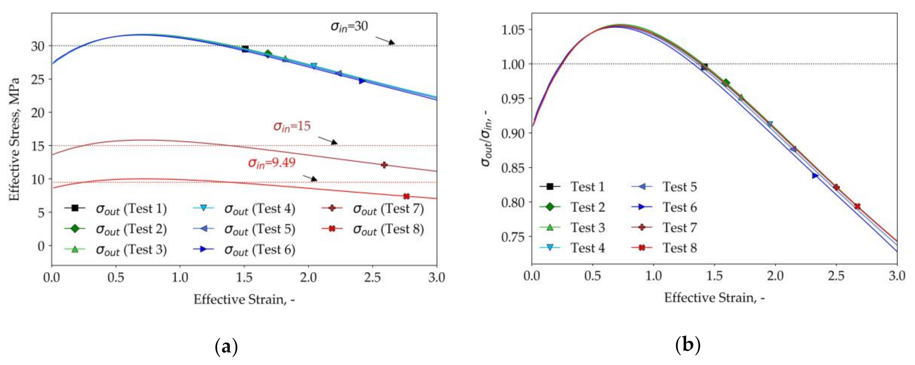
Figure 3 demonstrates the results of simulations with the different specimen and material parameters, which have an insignificant influence on the deviation of the output stress from the input one. The output stress–strain curves are presented in Figure 3a. Figure 3b presents the evolutions of the ratio between the output and input stresses.
The specimen thickness, which is not regulated by the ASTM standard, was variating within the range of 1.0 to 6.0 mm. The effect of friction was studied by evaluating the differences between the models with different friction coefficients. The effects of the material constant in the Backofen model and the nominal strain rate are also examined. The conditions of the eight tests illustrated in Figure 3 and the obtained deviations in the output stresses are presented in Table 1. The conditions of the reference test are provided in the first row. Other rows represent the tests with the variations of specimen thickness, friction coefficient, value, and the nominal strain rate. The effect of these variations was evaluated by the maximum deviation of the obtained output stress from the output stress corresponding to the reference test. The value of strain-rate sensitivity = 0.5 was used in all simulations.
When the Backofen model is used, the values of and the nominal strain rate should not affect the flow inhomogeneity and, subsequently, the deviations between the output and the input stresses. To demonstrate this fact, the output stress–strain curves corresponding to different values of and nominal strain rate are also presented in Figure 3a. As the variation of or nominal strain rate affects the input stress value, the evolution of the output stress value normalized to the input one () is more informative (Figure 3b). The results confirmed that the value of , as well as the nominal strain rate, does not affect the deviation of the output and input stresses.
The output stress deviations provided by the variation of thickness in the range of 1 to 6 mm do not exceed 1.95%. In the range of 1 to 4 mm, the deviations are less than 0.73%. Thus, it can be concluded that the specimen thickness has an insignificant effect on the results of tensile tests.
The deviations between the output stress evolutions, obtained in the tests with different friction values, are evaluated to study the effect of friction on the results of tensile testing. As can be observed in Table 1, these deviations are in the order of computational error and do not exceed 0.3%. As the material flow in the grip region is localized in the central area of a specimen, the slip of the specimen material over the grip shoulders is insignificant. Thus, friction has a neglectable effect on the results of tensile testing.
3.3. The Distributions of Strain Rate
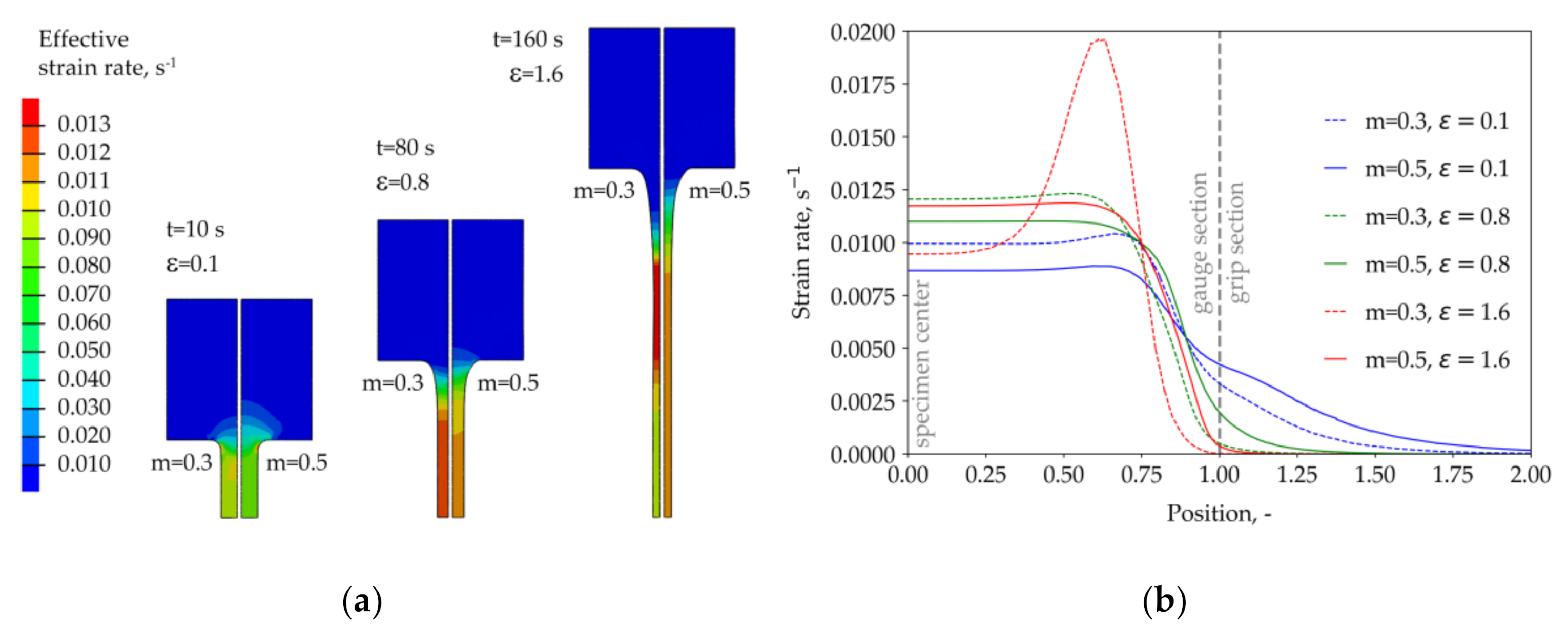
The distributions of strain rate within the specimen at different stages of the tensile process are presented in Figure 4 for two different values of : 0.3 and 0.5.
Figure 4a demonstrates the geometry of the deformed specimens with the distributions of the effective strain rate. At small deformations, the strain rates are localized near the corner adages of the gauge section. For the lower value, the average strain rate in the center is close to the nominal one. The larger value results in a lower strain rate in the center and deeper propagation of deformation to the grip section. At the nominal strain of 0.8, the maximum strain rates are observed in the central area of the grip region. The strain-rate inhomogeneity, as well as the maximum strain-rate value, are larger for the lower . Significant flow localization and the beginning of the necking process can be observed at the nominal strain of 1.6 for the lower value. The simulation with the value of equal to 0.5 does not demonstrate any necking effects at this nominal strain level.
The distributions of the effective strain rate along the central vertical axis of a specimen are presented in Figure 4b. Zero on the horizontal axis corresponds to the center of a specimen and 1 corresponds to the current position of the grip shoulders. The results obtained for the lower value are plotted by the dashed lines. Solid lines represent the results obtained for the higher . It can be seen that in the right side of the graph the solid lines are higher than the corresponding dashed ones. This indicates that the material flow from the grip region to the gauge area is more intensive at higher values of . Due to this effect, the deformation of the gauge section at the beginning of the test is slower than the one corresponding to the nominal strain rate.
The beginning of the necking process is reflected by the form of the dashed red line in Figure 4b. The maximum strain rate is two times higher than the one observed in the specimen center. All the other curves demonstrate almost uniform distributions of the strain rate in the central area, which covers about 75% of the gauge section. A local maximum of the blue dashed line corresponds to the initial strain-rate localization, which can be observed in Figure 4a on the specimen corresponding to = 0.3 and = 0.1. During further deformation, this initial localization degrades becoming almost invisible at = 0.8, but in the end, it provokes the nucleation of the necking process.
The strain rate in the central area continuously increases with the nominal deformation. The reason is that the width nonuniformity along the gauge section is not taken into account by the standard strain-rate control technique described by Equation (1). Equation (1) is derived from the assumption of the inverse proportion between the gauge length and the area of the central cross-section of the specimen. In reality, the cross-section area decreases faster, which is reflected in the increase in the strain-rate also reported in [18]. This process starts at the beginning of the test and continues until the necking.
3.4. The Effects of Material Properties on the Output Stress
3.4.1. Backofen Material Model
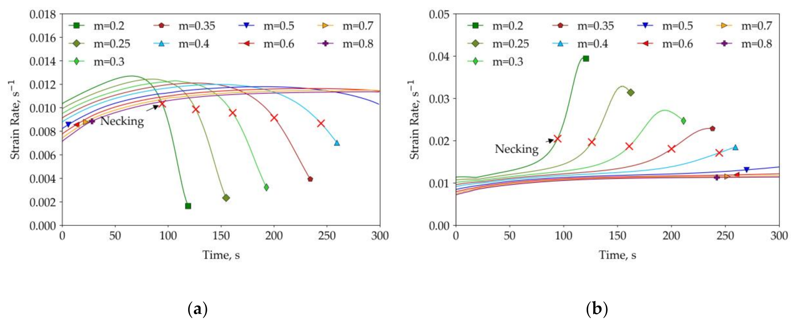
As the strain-rate sensitivity () is one of the most important characteristics of superplastic materials, which is responsible for flow localization and necking, the influence of the value on the output stress is in particular interest. Figure 5 shows how the value of in the Backofen equation affects the output stress. The value of was adjusted to the value in each simulation to keep the input stress at the level of 30 MPa at a strain rate of 10−2 s−1 (). This input stress value is plotted by the dotted line and denoted as . As the value of does not affect the strain-rate inhomogeneity, the differences in stress–strain behavior presented in Figure 5 are provided only by the variation of . It can be seen that the output stress at the beginning of the test is generally underestimated. With an increase in strain, the stress value increases until a certain peak level. Further increasing of the strain leads to decreasing of stress until the necking, which can be observed in the curves corresponding to lower values of as the sharp change in the curve slope.
In all tests presented in Figure 5, the necking occurred outside of the specimen center. The doubling of the maximum strain rate compared to the one corresponding to the specimen center was treated as the criteria of neck nucleation. The appropriate moments are marked by the red crosses. As can be observed in Figure 5, starting from these moments, the necking process becomes visible on the stress–strain curves. The effect of on the strain-rate evolution is illustrated in Figure 6. Figure 6a represents the evolutions of the maximum strain rate calculated along the central vertical axis. The necking process can be observed at lower values (less than 0.5) as the sharp rise in the maximum strain rate. The same process leads to the opposite effect in the specimen center as can be seen in Figure 6b. The strain rates increase until the neck nucleation after which the increase stops and the curve falls. In compliance with the Hart [24] stability analysis, higher values of results in later necking nucleation.
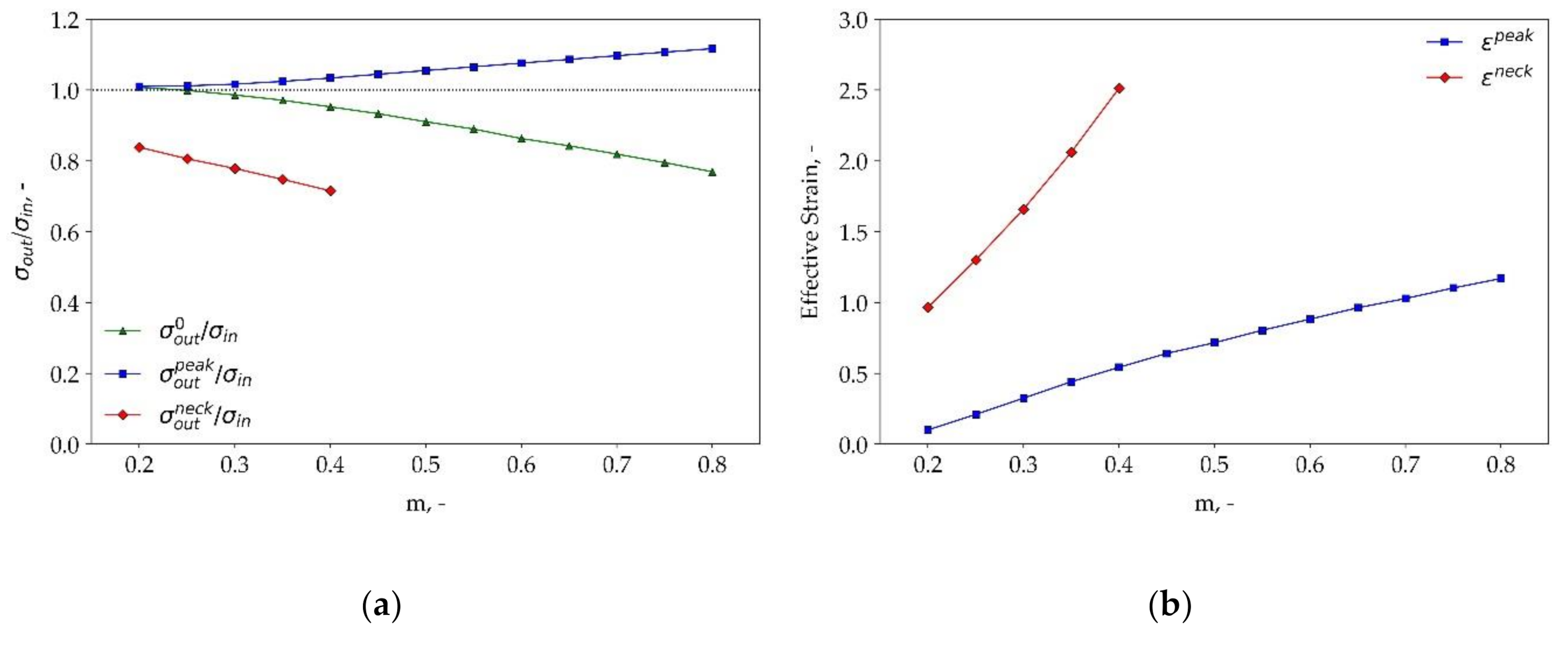
The appearance of the stress–strain curves illustrated in Figure 5 demonstrates that the errors produced by standard flow curve determination procedure depend significantly on the material strain-rate sensitivity. The higher values provide a significant underestimation of the effective stress at the beginning of deformation, while the lower ones result in a fake strain softening effect, which appears far before the necking is observable. To better illustrate these effects, the relations of the peak and necking stresses and strains, as well as the initial stresses on the value, are presented in Figure 7.
Figure 7a demonstrates the variations of the initial stress (), the peak stress (), and the necking stress () with the strain-rate sensitivity (). All values are normalized to the input stress value (). The apparent strain hardening effect is evaluated by the difference between the initial (blue curve) and the peak (green curve) stress, which increases from 0% of the target stress at = 0.2 to 21% at = 0.6 and 35% at = 0.8. The apparent strain softening effect (evaluated by the difference between and ) increases from 17% at = 0.2 to 32% at = 0.4.
Figure 7b demonstrates the variations of the peak strain () and the necking strain () with the value of . Both the strain hardening (zero to peak strain) and the strain softening (peak to necking strain) intervals become larger with the increase in the value. The relation of the necking stress on the value, plotted in Figure 7b by the red curve, qualitatively agrees with the experimental observations [1] and analytical predictions [24,31] of flow localization during tensile testing.
The results presented in this section are obtained for the ideal viscous material with the flow behavior described by the Backofen equation. It does not involve any local microstructural heterogeneities, cavitation, or fracture growth. The appearance of these effects during the deformation of real materials will result in earlier necking.
3.4.2. The Effect of Strain Hardening
To study the effect of strain hardening, Equation (6) was used in the simulations with equal to 300 and three values of (0.3, 0.5, and 0.7). The value of was varied in the range from 0.0 to 0.6 with a step of 0.1. The results are presented in Figure 8.
The output stress–strain curves obtained for = 0.5 and different values are plotted in Figure 8a by the solid lines. The dashed lines represent the input stress–strain relations. To study the difference between the input and the output stresses, the evolutions of input to output stress ratios are presented in Figure 8b for the same m value. Figure 8c,d demonstrate the same results for the values of equal to 0.3 and 0.7. As can be observed, the deviations between the input and the output stresses increase with strain hardening index. The moments corresponding to necking in Figure 8c are shifting to the right, demonstrating the increase in flow stability with the increase in strain hardening. The increase in strain hardening index results in the decrease in the normalized stress at the beginning of the test. The maximum value of the normalized stress is insignificantly affected by the value of the strain hardening index.
3.4.3. The Effect of Strain Rate
As shown above, if the material has flow behavior described by the Backofen model, the strain rate does not affect the flow inhomogeneity and the output stress accuracy. The strain-rate sensitivity in this case is invariant to strain rate. For the majority of superplastic materials, the strain-rate sensitivity varies with the strain rate. To study the effect of strain rate on the results of tensile testing, the material was described by Equation (5). Figure 9 illustrates the material properties presented by the relationship between stress and strain rate in a log–log scale (Figure 9a), and the relation of strain-rate sensitivity on the strain rate (Figure 9b). The stress vs. strain rate relation plotted in a log–log scale forms a sigmoidal curve with the inflection point corresponding to the strain rate, which provides the maximum value. This strain rate, which is referred to as the optimal one, provides the largest tensile elongations. The surrounding strain-rate range corresponding to values higher than 0.5 is referred to as the superplastic strain-rate range.
The simulations were performed for five referenced strain rates: one corresponding to the maximum and two pairs corresponding to m values of 0.3 and 0.5, as marked in Figure 9. The obtained stress–strain curves were compared with the ones obtained for Backofen approximations with similar values. Three of these approximations corresponding to the maximum and = 0.3 are plotted in Figure 9a by the dashed lines.
Figure 10a presents the output stress–strain curves obtained after FE simulations of the tensile tests of the materials described by the sigmoidal model (solid lines) and its Backofen approximations (dashed lines). The normalized strain evolutions are presented in Figure 10b. For each referenced strain rate, the input stress and the strain-rate sensitivity of the sigmoidal model are equal to the ones of the corresponding Backofen approximation. However, the output stress–strain relations are different because of the strain-rate inhomogeneity occurring during the tests. The most illustrative cases are the ones corresponding to = 0.3 ( and ). The strain-rate localization preceding the necking leads to an increase in strain rate, which in the case of lower nominal strain rate (), provides an increase in and subsequently better stability, slowing down the necking process. In the case of a higher strain rate, the same process provides lower values, accelerating necking. Thus, even though both nominal strain rates provide the same value equal to 0.3, the higher one results in earlier strain-rate localization and necking.
Equation (5) does not describe any strain hardening or softening during the deformation nor the variation of value with the effective strain. To evaluate the combined effect of these factors on the stress–strain curves obtained at different strain rates, the material model provided in [30] for the approximation of flow behavior of AA5083 alloy at 470 °C was used. The model is described by Equation (6). The results of these simulations are presented in Figure 11.
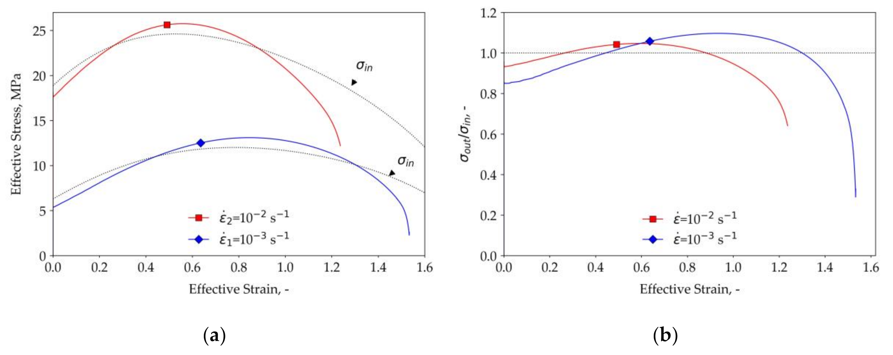
Figure 11a demonstrates the input stress–strain curves plotted by the dotted lines and compared with the output ones plotted by the solid lines. The input stress–strain relations demonstrate strain hardening at the beginning of the test and subsequent strain softening. Similar behavior is demonstrated by the output stress–strain curves. At the same time, both the strain hardening and the strain softening effects are overestimated in the output data. The evolution of the ratio between the output stress and the input stress is presented in Figure 11b. The initial stresses are underestimated by 7% for the higher strain rate and 15% for the lower one. The peak stresses are overestimated, respectively, by 5% and 10%. The lower strain rate provides larger elongation to necking than the higher strain rate.
3.5. Measurement of the Strain-Rate Sensitivity
ASTM E2448 standard suggests the step tensile test for the evaluation of the value [17]. During this test, the effective strain rate is periodically stepped to 20% above the nominal one and back. The steps are performed every 0.1 strain starting at 0.15. The value of strain-rate sensitivity index is then determined at each down step as:
where and are the effective stresses before and after the step, and and are the corresponding strain rates.
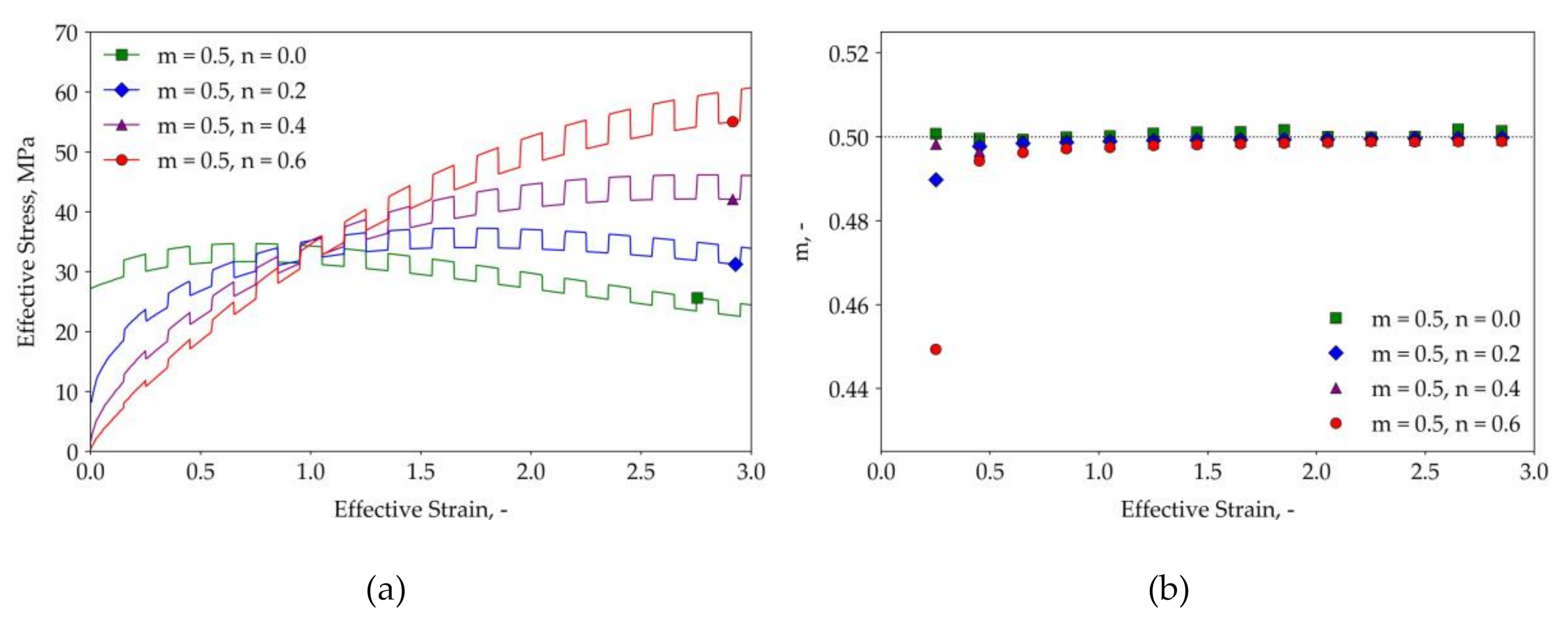
The results of step tensile tests for the material described by the power equation with different values are presented in Figure 12. Figure 12a demonstrates the stress–strain curves obtained by the step tests. The obtained values are presented in Figure 12b. The maximum error of value is 0.4% for the Backofen model ( = 0). For the higher values the decrease in accuracy is observed at the first step (maximum error of 10% is observed at = 0.6). The remaining steps demonstrate the errors that are less than 1%.
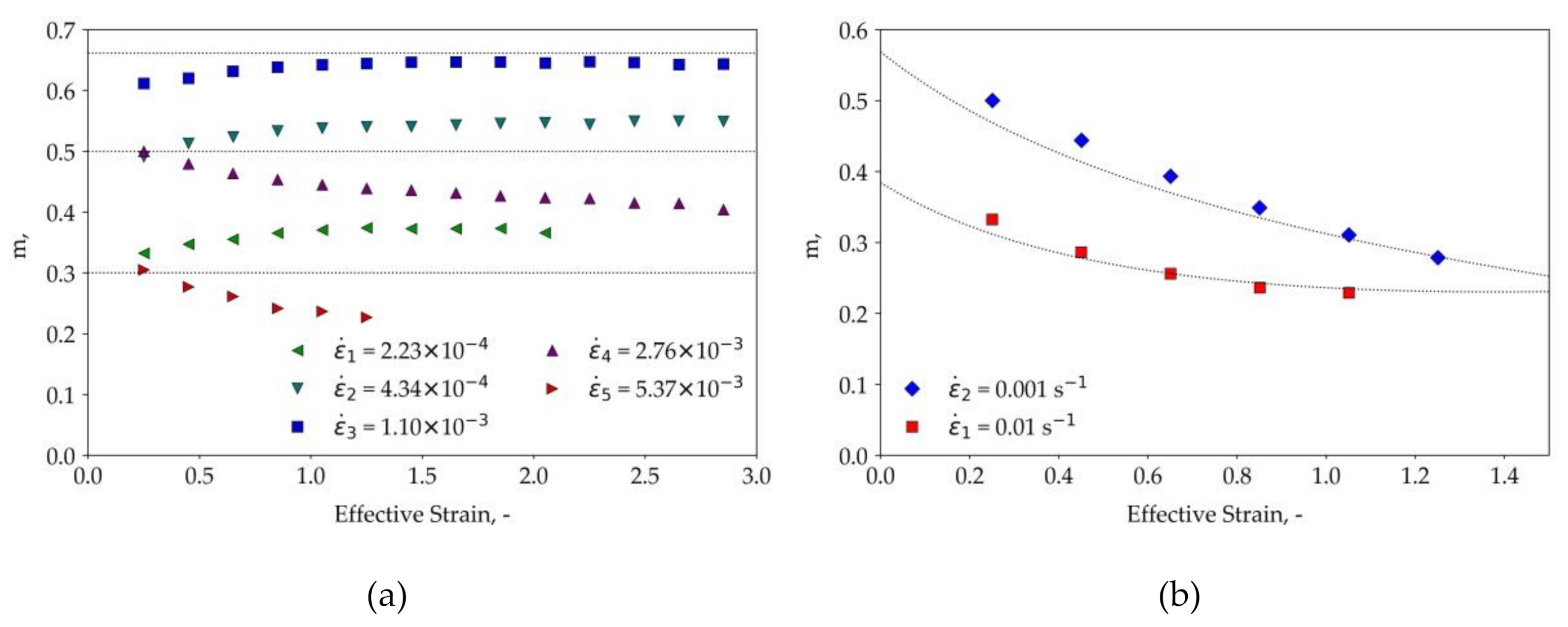
Larger errors are observed for the materials with a strain-rate-dependent value. The strain-rate sensitivity values for the materials described by Equations (5) and (6), determined based on the standard technique, are presented in Figure 13. The output values of are plotted by markers, while the values corresponding to the input constitutive model are plotted by dotted lines. Figure 13a demonstrates the relations of value on the effective stress for the material model described by Equation (5). It can be observed that the output value increases with the effective strain at the lower strain rates and decreases at the higher ones. This behavior is consistent with the strain-rate evolution taking place during tensile testing. If the strain rate is lower than the one corresponding to maximum , then the increase in the actual strain rate during the test leads to an increase in the corresponding values, as can be observed in Figure 9b. For the higher strain rates, the opposite effect is observed.
The test at the strain rate corresponding to the maximum provides slightly underestimated output values. The largest error corresponds to the first step and equals 7.5%. The errors provided by the other tests increase with the strain. The lower strain rates provide overestimated values of . The errors increase from the neglectable values at the first step, reaching 25% (for ) and 8% (for ) at the strain equal to 1.25. The opposite behavior is demonstrated at the higher strain rates: the m values are underestimated, and the errors at the effective strain of 1.25 reach 12% (for ) and 25% (for ).
The output values of corresponding to the material model described by Equation (6) are presented in Figure 13b. The obtained strain-rate sensitivity is slightly overestimated at the beginning of the test. The maximum errors are 7.4% for the lower strain rate and 6.6% for the higher strain rate.
4. Discussion
The performed FE simulations of a superplastic tensile test revealed that the inhomogeneity of the strain rate within the specimen volume and its variation in time significantly affects the accuracy of the resulting strain-stress curves. The standard procedure of the calculation of stresses and strains provides regular errors that depend on the material properties. Generally, two major aspects affect these errors: the material flow from the grip region to the gauge section and the non-uniform thinning of the gauge section.
The material flow from the gauge section is considered as one of the main sources of errors during the superplastic tensile test. The results presented in Figure 4 show that this effect is more significant for the materials with a larger value. The most intensive material flow from the grip region is observed at the beginning of the test. As a result, the strain rates in the gauge section become slower. Thus, the output stresses corresponding to the materials with larger values are generally underestimated at the beginning of the test. The larger provides a larger initial underestimation of the stress. The material flow from the grip region is weakening with deformation, which results in the increase in the strain rate and subsequent increase in output stress. Thus, the strain hardening effect is generally overestimated at the low strains.
Another source of the increase in strain rate is the nonuniformity of the width and thickness reduction in the gauge section and the subsequent nonuniformity of the effective strain. As shown in Section 3.3, for the investigated specimen geometry, only 75% of the gauge section is deformed uniformly, while the grip velocity is adjusted based on the assumption of uniform deformation in the entire gauge region. Thus, the minimum cross-section area is reduced faster than assumed in the standard procedure.
While the increase in the strain rate leads to the increasing overestimation of the output stress, the rapid reduction in the minimum cross-section has the opposite effect. Thus, the output stress–strain curves obtained for the Backofen model demonstrate strain softening at the larger strains. A similar effect is taking place for the material with more complex constitutive behavior: the standard tensile testing procedure tends to overestimate the strain hardening effect at the low strains and the strain softening effect at the higher ones.
The effects of strain hardening or softening give important information about the material, as they are usually associated with the microstructure processes, such as grain growth or dynamic recrystallization. The results presented in this paper show that even if the material behavior does not demonstrate any strain hardening or softening effects, they will appear in the stress–strain curve obtained by the standard tensile testing procedure. These effects do not reflect the material behavior at a constant strain rate. They are resulting from the flow inhomogeneity during the tensile test and reflecting the errors provided by the standard procedure of superplastic tensile testing.
5. Concluding Remarks
The material properties significantly affect the accuracy of the stress–strain curves obtained by standard superplastic tensile tests. The influence of material behavior on the specimen forming during the test, and the subsequent stress–strain curve, is associated with the following effects:
- Higher strain-rate sensitivity values provide lower initial output stresses and larger apparent strain hardening effect.
- Apparent strain softening effect occurs long before the observable necking of a specimen.
- Equal values of the strain-rate sensitivity index do not guarantee equal elongations prior to necking, if the strain-rate sensitivity is strain-rate-dependent. In particular, if the material behavior is described by the sigmoidal log stress vs. log strain rate relation, higher elongations are produced by the lower strain rate associated with the same strain-rate sensitivity.
- A larger variation of strain-rate sensitivity with the strain rate provides larger errors in the determination of . For the strain rates corresponding to the edges of the quasi-SPF strain-rate range, this error may reach 25%. Lower variations of provide lower errors, which become neglectable if the material flow behavior follows the Backofen power law.
- The variation of friction between the specimen and the grip shoulders and the initial specimen thickness has an insignificant effect on the evolution of output stress in tensile testing.
The effects listed above should be taken into account during the analysis of the stress–strain data obtained by tensile testing. As these data are not measured directly during the tests, their accuracy should be checked by numerical simulations and, if necessary, refined by an inverse analysis.
Author Contributions
Conceptualization, S.A.; methodology, S.A. and V.M.; software, V.M.; validation, S.A. and V.M.; formal analysis, S.A. and V.M.; writing—original draft preparation, S.A.; writing—review and editing, S.A. and V.M.; visualization, V.M. All authors have read and agreed to the published version of the manuscript.
Funding
This research was performed in the framework of the project (order No.2.10—5/2905-01 from 29.05.2020) coordinated by Prof. Popov and supported by the Scientific Committee of the Faculty of Business and Management of National Research University Higher School of Economics (protocol No.4 from 18.06.2020).
Conflicts of Interest
The authors declare no conflict of interest.
References
- Langdon, T.G. The mechanical properties of superplastic materials. Metall. Trans. A 1982, 13, 689–701. [Google Scholar] [CrossRef]
- Sherby, O.D.; Wadsworth, J. Superplasticity—Recent advances and future directions. Prog. Mater. Sci. 1989, 33, 169–221. [Google Scholar] [CrossRef]
- Enikeev, F.; Kruglov, A. An analysis of the superplastic forming of a thin circular diaphragm. Int. J. Mech. Sci. 1995, 37, 473–483. [Google Scholar] [CrossRef]
- Giuliano, G.; Franchitti, S. On the evaluation of superplastic characteristics using the finite element method. Int. J. Mach. Tools Manuf. 2007, 47, 471–476. [Google Scholar] [CrossRef]
- Aksenov, S.A.; Chumachenko, E.N.; Kolesnikov, A.V.; Osipov, S.A. Determination of optimal gas forming conditions from free bulging tests at constant pressure. J. Mater. Process. Technol. 2015, 217, 158–164. [Google Scholar] [CrossRef]
- Guglielmi, P.; Sorgente, D.; Lombardi, A.; Palumbo, G. A new experimental approach for modelling the constitutive behaviour of sheet metals at elevated temperature through interrupted bulge tests. Int. J. Mech. Sci. 2020, 184, 105839. [Google Scholar] [CrossRef]
- Vulcan, M.; Siegert, K.; Banabic, D. The Influence of Pulsating Strain Rates on the Superplastic Deformation Behaviour of Al-Alloy AA5083 Investigated by Means of Cone Test. Mater. Sci. Forum 2004, 447–448, 139–144. [Google Scholar] [CrossRef]
- El-Morsy, A.; Akkus, N.; Manabe, K.; Nishimura, H. Evaluation of superplastic characteristics of tubular materials by multi-tube bulge test. Mater. Lett. 2006, 60, 559–564. [Google Scholar] [CrossRef]
- Alabort, E.; Putman, D.; Reed, R.C. Superplasticity in Ti–6Al–4V: Characterisation, modelling and applications. Acta Mater. 2015, 95, 428–442. [Google Scholar] [CrossRef] [Green Version]
- Yasmeen, T.; Shao, Z.; Zhao, L.; Gao, P.; Lin, J.; Jiang, J. Constitutive modeling for the simulation of the superplastic forming of TA15 titanium alloy. Int. J. Mech. Sci. 2019, 164, 105178. [Google Scholar] [CrossRef]
- Shen, J.; Sun, Y.; Ning, Y.; Yu, H.; Yao, Z.; Hu, L. Superplasticity induced by the competitive DRX between BCC beta and HCP alpha in Ti-4Al-3V-2Mo-2Fe alloy. Mater. Charact. 2019, 153, 304–317. [Google Scholar] [CrossRef]
- Yang, J.; Wu, J.; Zhang, Q.; Han, R.; Wang, K. Investigation of flow behavior and microstructure of Ti–6Al–4V with annealing treatment during superplastic forming. Mater. Sci. Eng. A 2020, 797, 140046. [Google Scholar] [CrossRef]
- Guan, Z.; Ren, M.; Zhao, P.; Ma, P.; Wang, Q. Constitutive equations with varying parameters for superplastic flow behavior of Al-Zn-Mg-Zr alloy. Mater. Des. 2014, 54, 906–913. [Google Scholar] [CrossRef]
- Chumachenko, E.N.; Portnoi, V.K.; Paris, L.; Billaudeau, T. Analysis of the SPF of a titanium alloy at lower temperatures. J. Mater. Process. Technol. 2005, 170, 448–456. [Google Scholar] [CrossRef]
- Gao, F.; Li, W.; Meng, B.; Wan, M.; Zhang, X.; Han, X. Rheological law and constitutive model for superplastic deformation of Ti-6Al-4V. J. Alloys Compd. 2017, 701, 177–185. [Google Scholar] [CrossRef]
- Mosleh, A.O.; Mikhaylovskaya, A.V.; Kotov, A.D.; Kwame, J.S. Experimental, modelling and simulation of an approach for optimizing the superplastic forming of Ti-6%Al-4%V titanium alloy. J. Manuf. Process. 2019, 45, 262–272. [Google Scholar] [CrossRef]
- E2448-11 Standard Test Method for Determining the Superplastic Properties of Metallic Sheet Materials; ASTM B. Standards: West Conshohocken, PA, USA, 2011. [CrossRef]
- Khaleel, M.A.; Johnson, K.I.; Lavender, C.A.; Smith, M.T.; Hamilton, C.H. Specimen geometry effect on the accuracy of constitutive relations in a superplastic 5083 aluminum alloy. Scr. Mater. 1996, 34, 1417–1423. [Google Scholar] [CrossRef]
- Sorgente, D.; Tricarico, L. Analysis of Different Specimen Geometries for Tensile Tests in Superplastic Conditions for an Aluminium Alloy. Mater. Sci. Forum 2007, 551–552, 123–128. [Google Scholar] [CrossRef]
- Abu-Farha, F.K.; Khraisheh, M.K. On the High Temperature Testing of Superplastic Materials. J. Mater. Eng. Perform. 2007, 16, 142–149. [Google Scholar] [CrossRef]
- Bate, P.S.; Ridley, N.; Sotoudeh, K. Effect of gauge length in superplastic tensile tests. Mater. Sci. Technol. 2008, 24, 1265–1270. [Google Scholar] [CrossRef]
- Abu-Farha, F.; Nazzal, M.; Curtis, R. Optimum Specimen Geometry for Accurate Tensile Testing of Superplastic Metallic Materials. Exp. Mech. 2011, 51, 903–917. [Google Scholar] [CrossRef]
- Nazzal, M.; Abu-Farha, F.; Curtis, R. Finite Element Simulations for Investigating the Effects of Specimen Geometry in Superplastic Tensile Tests. J. Mater. Eng. Perform. 2011, 20, 865–876. [Google Scholar] [CrossRef]
- Hart, E. Theory of the tensile test. Acta Metall. 1967, 15, 351–355. [Google Scholar] [CrossRef]
- Langdon, T.G. Forty-Five Years of Superplastic Research: Recent Developments and Future Prospects. Mater. Sci. Forum 2016, 838, 3–12. [Google Scholar] [CrossRef]
- Yang, W.; Guo, X.; Yang, K. Low temperature quasi-superplasticity of ZK60 alloy prepared by reciprocating extrusion. Trans. Nonferrous Met. Soc. China 2012, 22, 255–261. [Google Scholar] [CrossRef]
- Vasin, R.A.; Enikeev, F.U.; Mazurski, M.I.; Munirova, O.S. Mechanical modelling of the universal superplastic curve. J. Mater. Sci. 2000, 35, 2455–2466. [Google Scholar] [CrossRef]
- Smirnov, O.M. Rheological Behavior of Superplastic Nanocrystalline and Amorphous Materials. Mater. Sci. Forum 1999, 304, 341–348. [Google Scholar] [CrossRef]
- Aksenov, S.; Chumachenko, E.; Logashina, I. Experimental investigation of Ti-Al-V alloy superplastic behavior. In Proceedings of the METAL 2012—Conference Proceedings, 21st International Conference on Metallurgy and Material, Brno, Czech Republic, 23–25 May 2012. [Google Scholar]
- Majidi, O.; Jahazi, M.; Bombardier, N. A viscoplastic model based on a variable strain rate sensitivity index for superplastic sheet metals. Int. J. Mater. Form. 2019, 12, 693–702. [Google Scholar] [CrossRef]
- Chinh, N.Q.; Rácz, G.; Gubicza, J.; Valiev, R.Z.; Langdon, T.G. A possible stabilizing effect of work hardening on the tensile performance of superplastic materials. Mater. Sci. Eng. A 2019, 759, 448–454. [Google Scholar] [CrossRef]
Figure 1.
The computer model of tensile test: (a) geometry of a specimen; (b) Finite element meshes used in the simulations.
Figure 1.
The computer model of tensile test: (a) geometry of a specimen; (b) Finite element meshes used in the simulations.

Figure 2.
The effect of finite element mesh and the way of force calculation on the output stress–strain curve: (a) for the box geometry realizing the ideal uniaxial tension conditions; (b) for the real specimen geometry.
Figure 2.
The effect of finite element mesh and the way of force calculation on the output stress–strain curve: (a) for the box geometry realizing the ideal uniaxial tension conditions; (b) for the real specimen geometry.

Figure 3.
The effect of the specimen thickness, friction coefficient, nominal strain rate, and the value of on the tensile test results for the material described by the Backofen model: (a) the output stress–strain curves; (b) the normalized output stress () vs. strain curves.
Figure 3.
The effect of the specimen thickness, friction coefficient, nominal strain rate, and the value of on the tensile test results for the material described by the Backofen model: (a) the output stress–strain curves; (b) the normalized output stress () vs. strain curves.

Figure 4.
The results of simulations of tensile testing performed using two different values of : (a) the distributions of strain rate within the deformed specimens; (b) the distributions of strain rate along the central axis of a specimen.
Figure 4.
The results of simulations of tensile testing performed using two different values of : (a) the distributions of strain rate within the deformed specimens; (b) the distributions of strain rate along the central axis of a specimen.

Figure 5.
The effect of strain-rate sensitivity () on the stress–strain curves obtained by tensile testing.
Figure 5.
The effect of strain-rate sensitivity () on the stress–strain curves obtained by tensile testing.
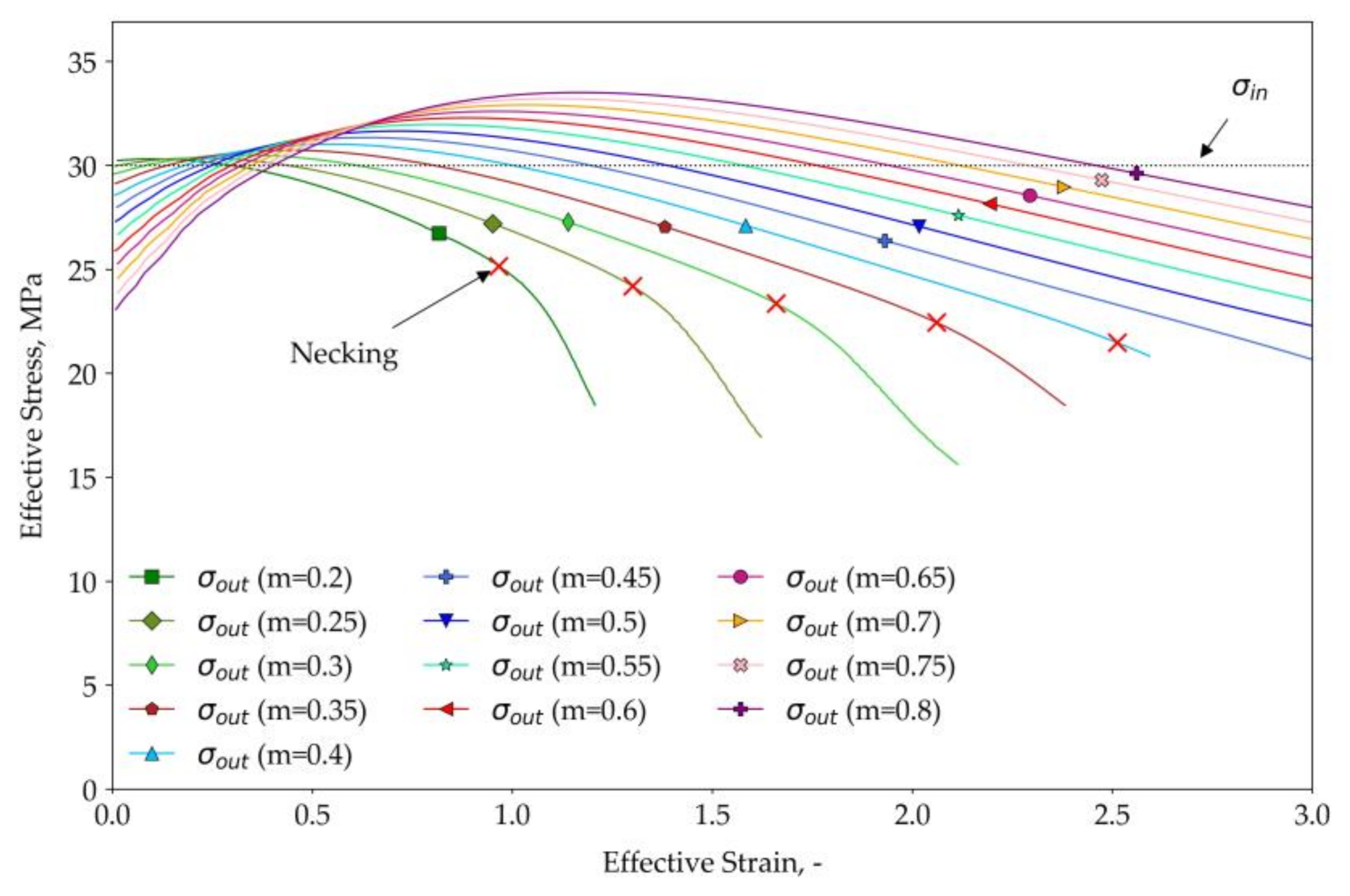
Figure 6.
The effect of strain-rate sensitivity () on the strain-rate evolution: (a) the evolutions of the strain rate in the specimen center obtained for different values; (b) the evolutions of the maximum strain rate for different values.
Figure 6.
The effect of strain-rate sensitivity () on the strain-rate evolution: (a) the evolutions of the strain rate in the specimen center obtained for different values; (b) the evolutions of the maximum strain rate for different values.

Figure 7.
The effect of strain-rate sensitivity () on the apparent strain hardening and softening: (a) the initial, peak, and necking stresses related to the value; (b) the relations of the peak strain and the necking strain on the value.
Figure 7.
The effect of strain-rate sensitivity () on the apparent strain hardening and softening: (a) the initial, peak, and necking stresses related to the value; (b) the relations of the peak strain and the necking strain on the value.

Figure 8.
The effect of strain hardening () on the results of tensile testing: (a) the stress–strain curves obtained for different values at ; (b) the normalized stress evolutions for ; (c) the normalized stress evolutions for ; (d) the normalized stress evolutions for .
Figure 8.
The effect of strain hardening () on the results of tensile testing: (a) the stress–strain curves obtained for different values at ; (b) the normalized stress evolutions for ; (c) the normalized stress evolutions for ; (d) the normalized stress evolutions for .
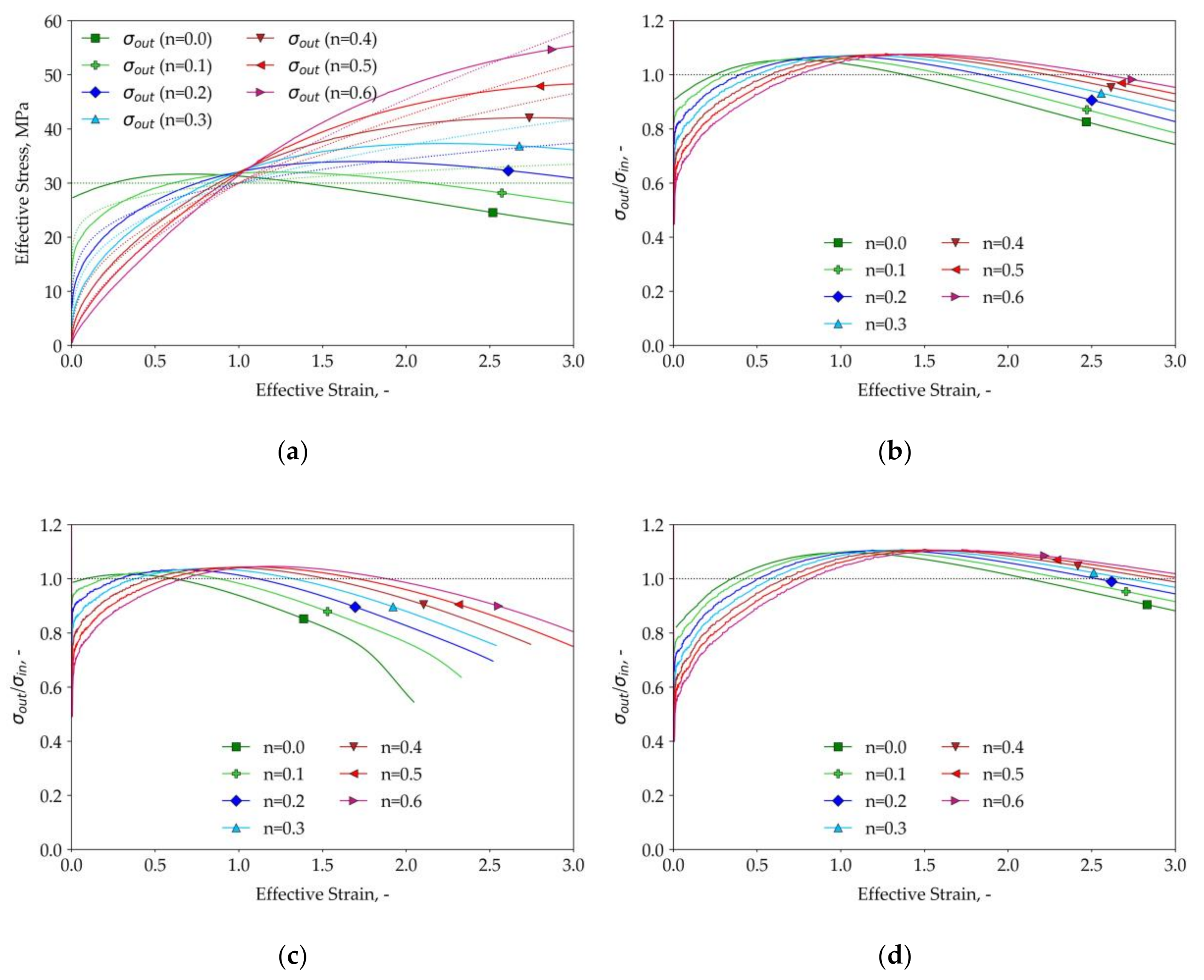
Figure 9.
A sigmoidal material model and the strain rates used in the simulations: (a) the relation between the stress and strain (solid) and the Backofen approximations for three selected strain rates (dashed) plotted in logarithmic scale; (b) the relation of strain-rate sensitivity index on the effective strain rate.
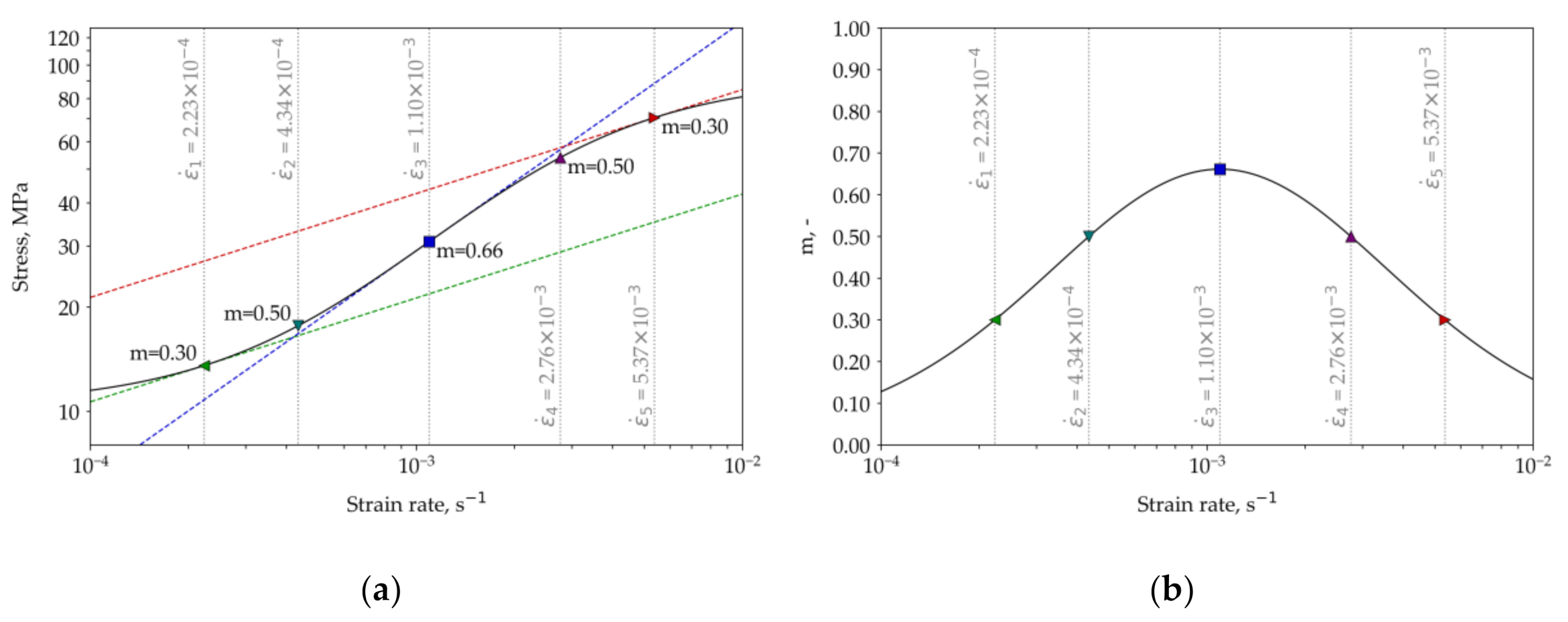
Figure 10.
The effect of strain rate on the stress–strain curves obtained by tensile testing: (a) the stress–strain curves obtained for different strain rates using the sigmoidal material model (solid) and its Backofen approximations (dashed); (b) the normalized stress evolutions obtained for different strain rates using the sigmoidal material model.
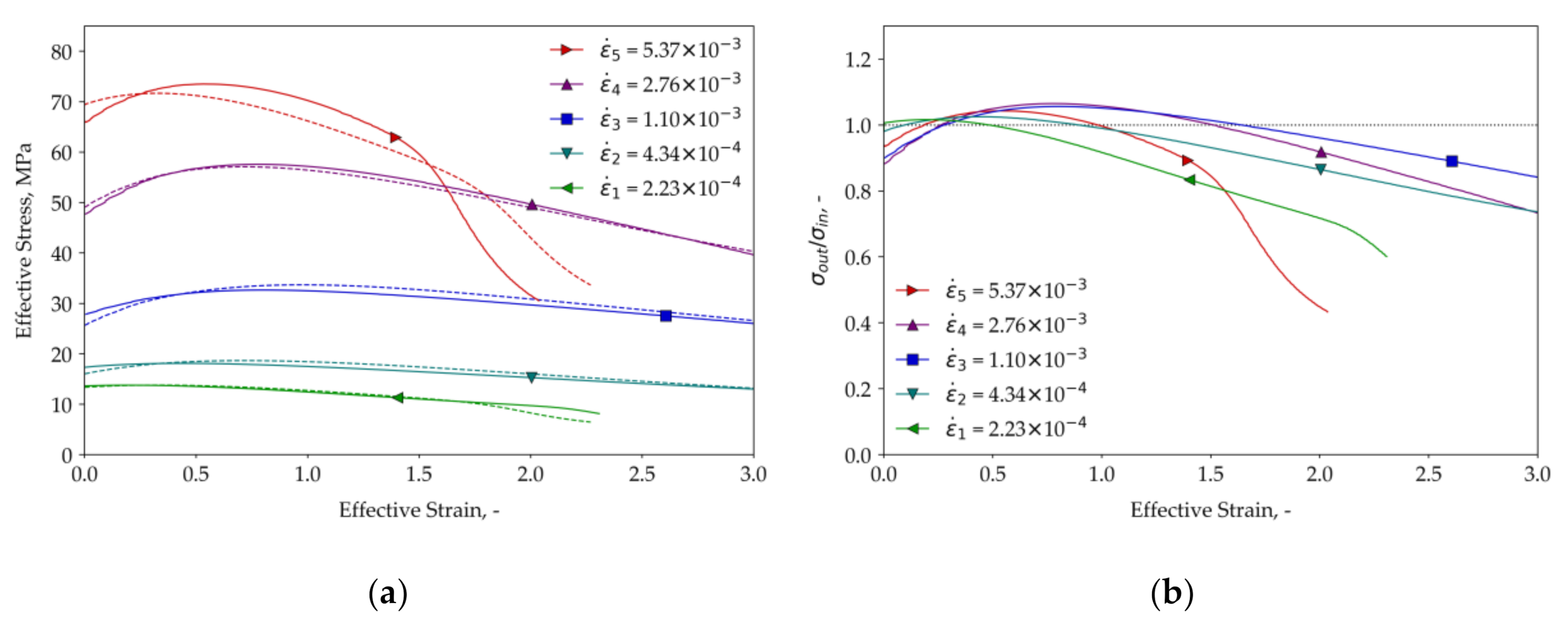
Figure 11.
The relations of the input and the output stress on the effective strain for the material model described by Equation (6): (a) the stress–strain curves for two different strain rates; (b) the normalized stress evolution for two different strain rates.
Figure 11.
The relations of the input and the output stress on the effective strain for the material model described by Equation (6): (a) the stress–strain curves for two different strain rates; (b) the normalized stress evolution for two different strain rates.

Figure 12.
The simulation of the step tests aimed to determine the value: (a) the stress–strain curves corresponding to the step tests for the material with = 0.5 and different values; (b) the obtained values of strain-rate sensitivity index () related to the effective strain.
Figure 12.
The simulation of the step tests aimed to determine the value: (a) the stress–strain curves corresponding to the step tests for the material with = 0.5 and different values; (b) the obtained values of strain-rate sensitivity index () related to the effective strain.

Figure 13.
The relations of value on the effective strain at different strain rates: (a) for the sigmoidal material model (Equation (5)); (b) for the material model described by Equation (6).
Figure 13.
The relations of value on the effective strain at different strain rates: (a) for the sigmoidal material model (Equation (5)); (b) for the material model described by Equation (6).


Table 1.
The conditions of the tests and the deviations in output stress reflecting the variation of specimen thickness, friction coefficient, nominal strain rate, and the value of .
Table 1.
The conditions of the tests and the deviations in output stress reflecting the variation of specimen thickness, friction coefficient, nominal strain rate, and the value of .
| Number | Initial Thickness | Friction Coefficient | Nominal Strain Rate | Deviation of the Output Stress | |
|---|---|---|---|---|---|
| 1 | 1 mm | 0.4 | 0.01 s−1 | 300 | reference test |
| 2 | 1 mm | 0.0 | 0.01 s−1 | 300 | 0.26% |
| 3 | 1 mm | 0.2 | 0.01 s−1 | 300 | 0.18% |
| 4 | 2 mm | 0.4 | 0.01 s−1 | 300 | 0.09% |
| 5 | 4 mm | 0.4 | 0.01 s−1 | 300 | 0.73% |
| 6 | 6 mm | 0.4 | 0.01 s−1 | 300 | 1.95% |
| 7 | 1 mm | 0.4 | 0.01 s−1 | 150 | 0.05% |
| 8 | 1 mm | 0.4 | 0.001 s−1 | 300 | 0.08% |
© 2020 by the authors. Licensee MDPI, Basel, Switzerland. This article is an open access article distributed under the terms and conditions of the Creative Commons Attribution (CC BY) license (http://creativecommons.org/licenses/by/4.0/).
Share and Cite
MDPI and ACS Style
Aksenov, S.; Mikolaenko, V. The Effect of Material Properties on the Accuracy of Superplastic Tensile Test. Metals 2020, 10, 1353. https://doi.org/10.3390/met10101353
AMA Style
Aksenov S, Mikolaenko V. The Effect of Material Properties on the Accuracy of Superplastic Tensile Test. Metals. 2020; 10(10):1353. https://doi.org/10.3390/met10101353
Chicago/Turabian StyleAksenov, Sergey, and Vadim Mikolaenko. 2020. "The Effect of Material Properties on the Accuracy of Superplastic Tensile Test" Metals 10, no. 10: 1353. https://doi.org/10.3390/met10101353
Note that from the first issue of 2016, this journal uses article numbers instead of page numbers. See further details here.