Analysis of Wind Data for Sports Performance Design: A Case Study for Sailing Sports


Abstract
:1. Introduction
- (1)
- wind varies in the different zones both in direction and speed;
- (2)
- wind varies in the different zones for direction and not for intensity (these regatta fields are extremely rare);
- (3)
- wind intensity varies and wind direction remains almost constant (or also there is a variation of the “wind pressure”).
2. Material and Methods
2.1. Research Design
2.2. Material
2.2.1. The CALMET Meteorological Model
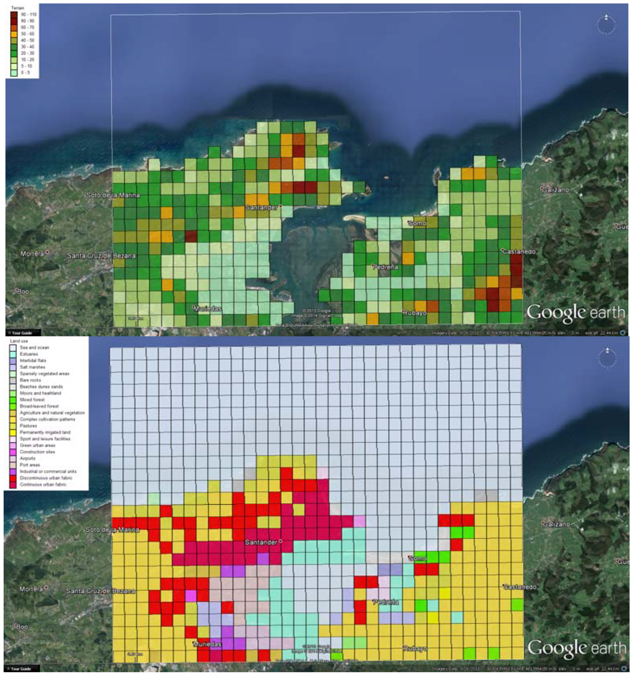
2.2.2. Geophysical Data
2.2.3. Input Meteorological Data


2.2.4. The WindRose PRO3 Software
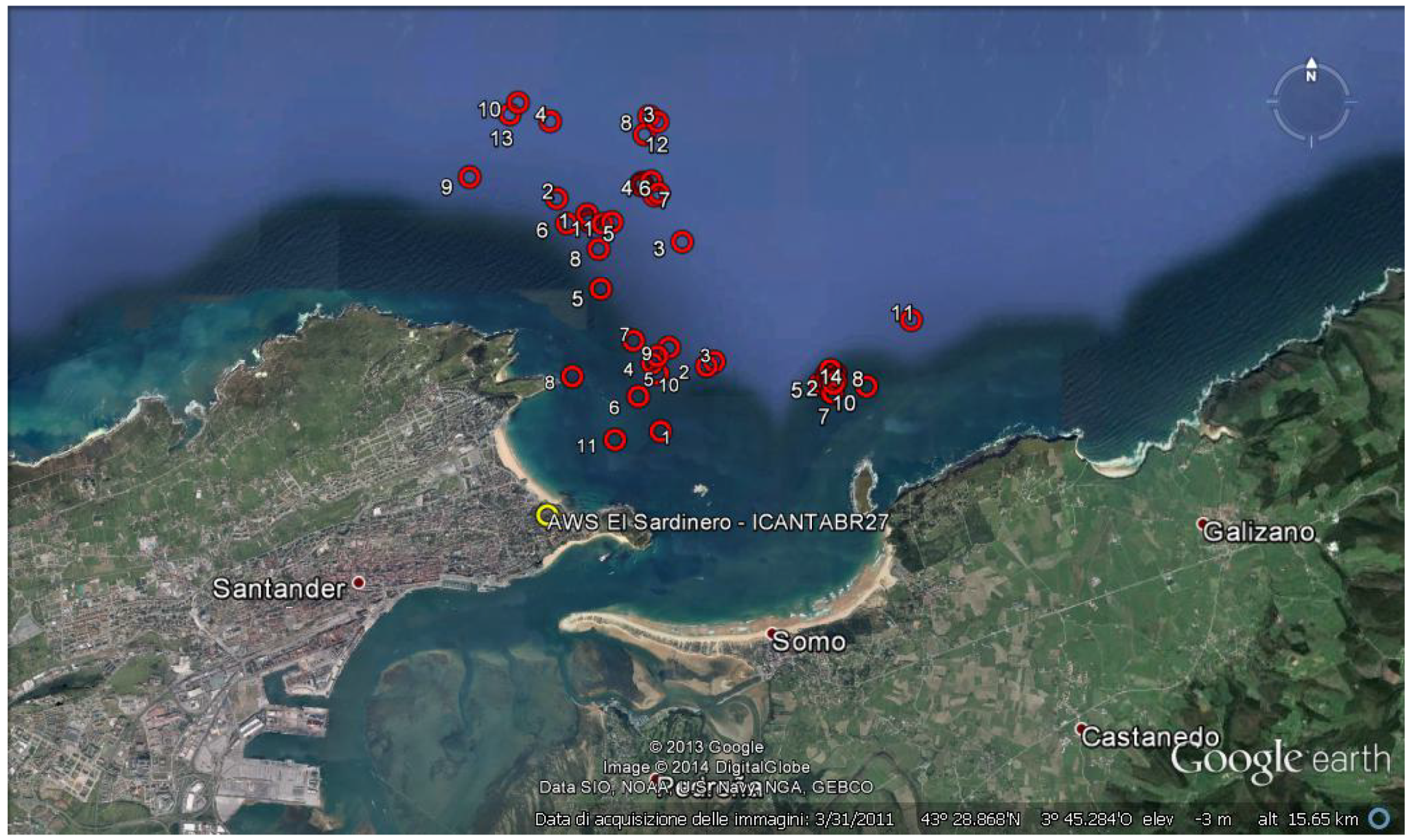
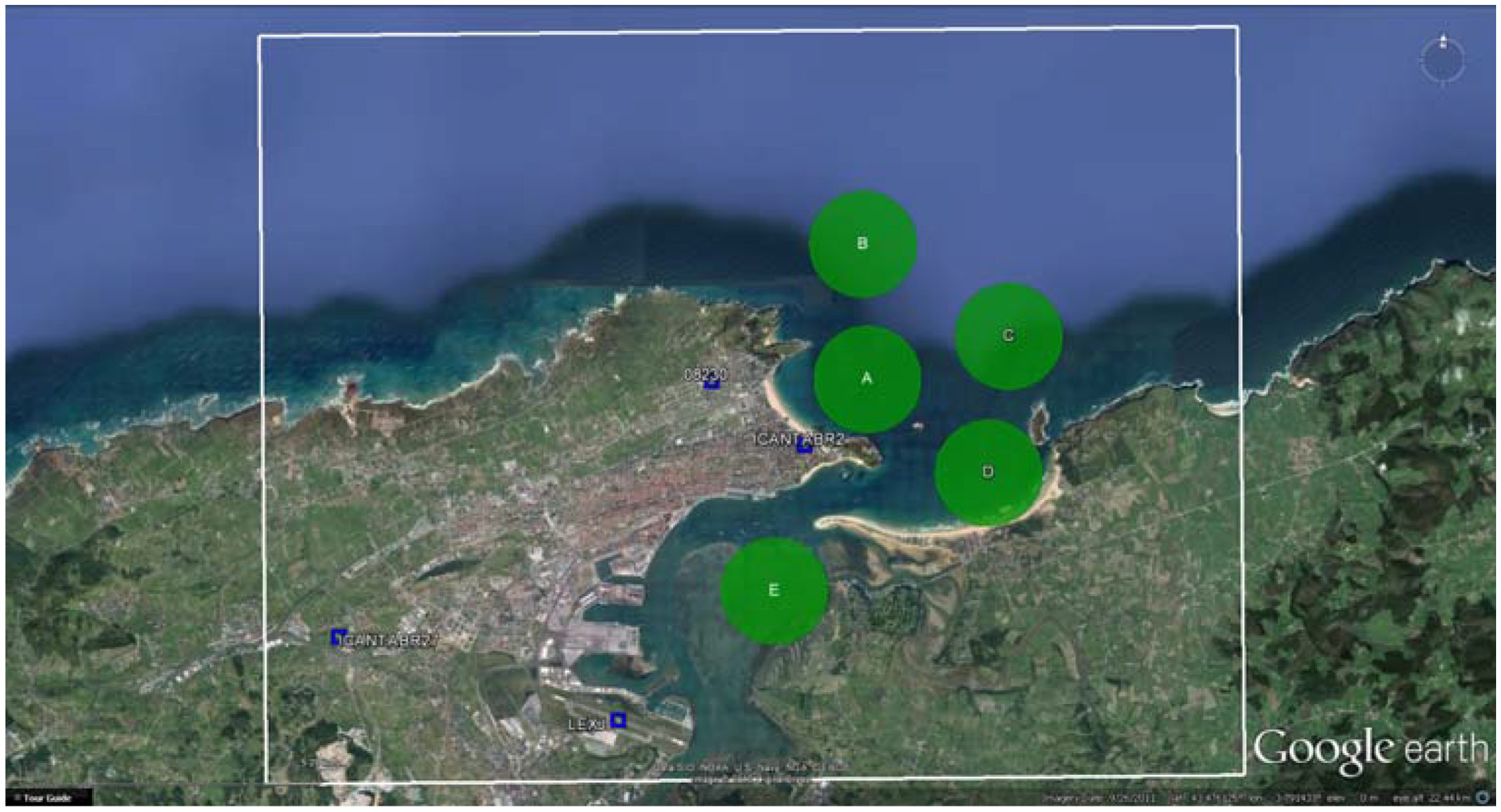
2.2.5. Off Shore Weather Observations
2.3. Methods
2.3.1. Weather Patterns
2.3.2. Comparison against the Observations
2.3.3. Use of the CALMET Results for Creating the “Call Book”
3. Results and Discussion
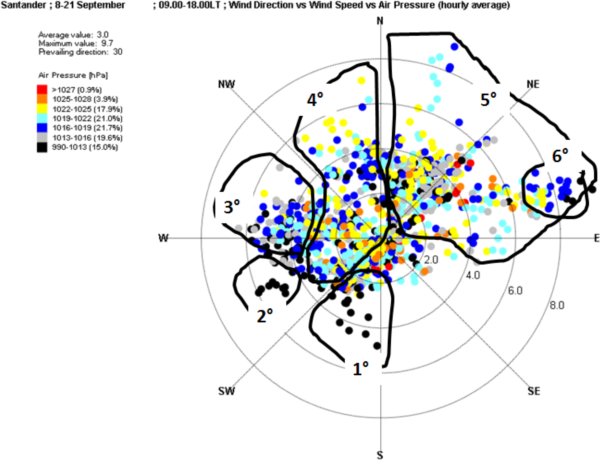
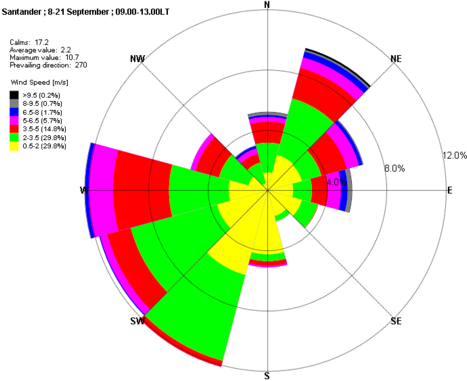
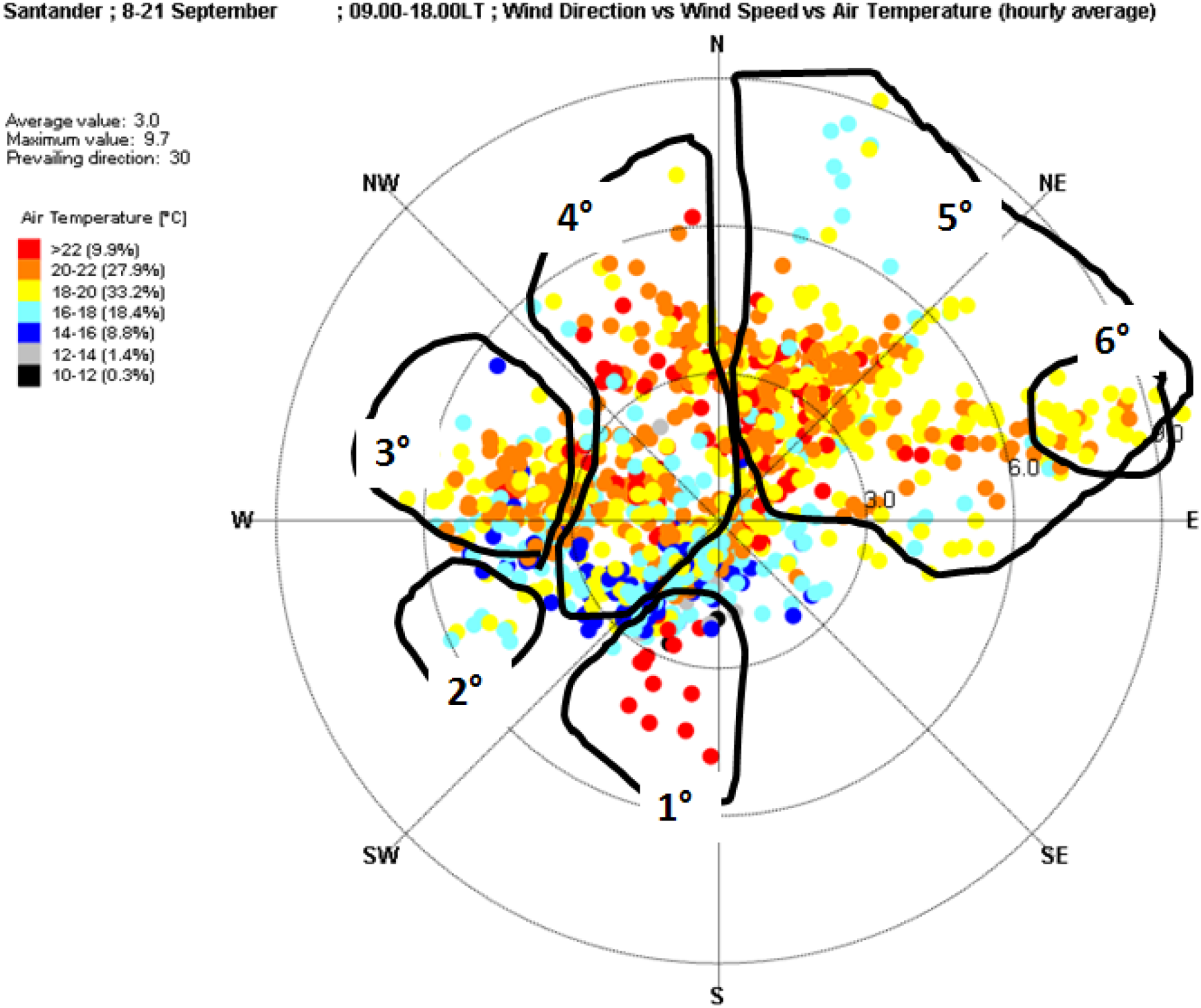
3.1. Weather Patterns
- (1)
- Wind from S-SSW. Pre-frontal situation (gradient from SSW), not frequent (5%), warm wind prevailing during the morning which rapidly rotates toward SW decreasing atmospheric pressure and increasing wind speed.
- (2)
- Wind from SW. Classic pre-frontal and frontal situation (gradient from SW), not frequent if analyzed alone (5%). Generally it is associated to pattern 3 since the atmospheric pressure rapidly increases as the front passes and wind rotates to W-NW. The wind from SW is stable until the passage of the front. The same pattern is presented by the land thermal from SW, which rotates to NE during the day (it is characterized by high atmospheric pressure and low wind intensity).
- (3)
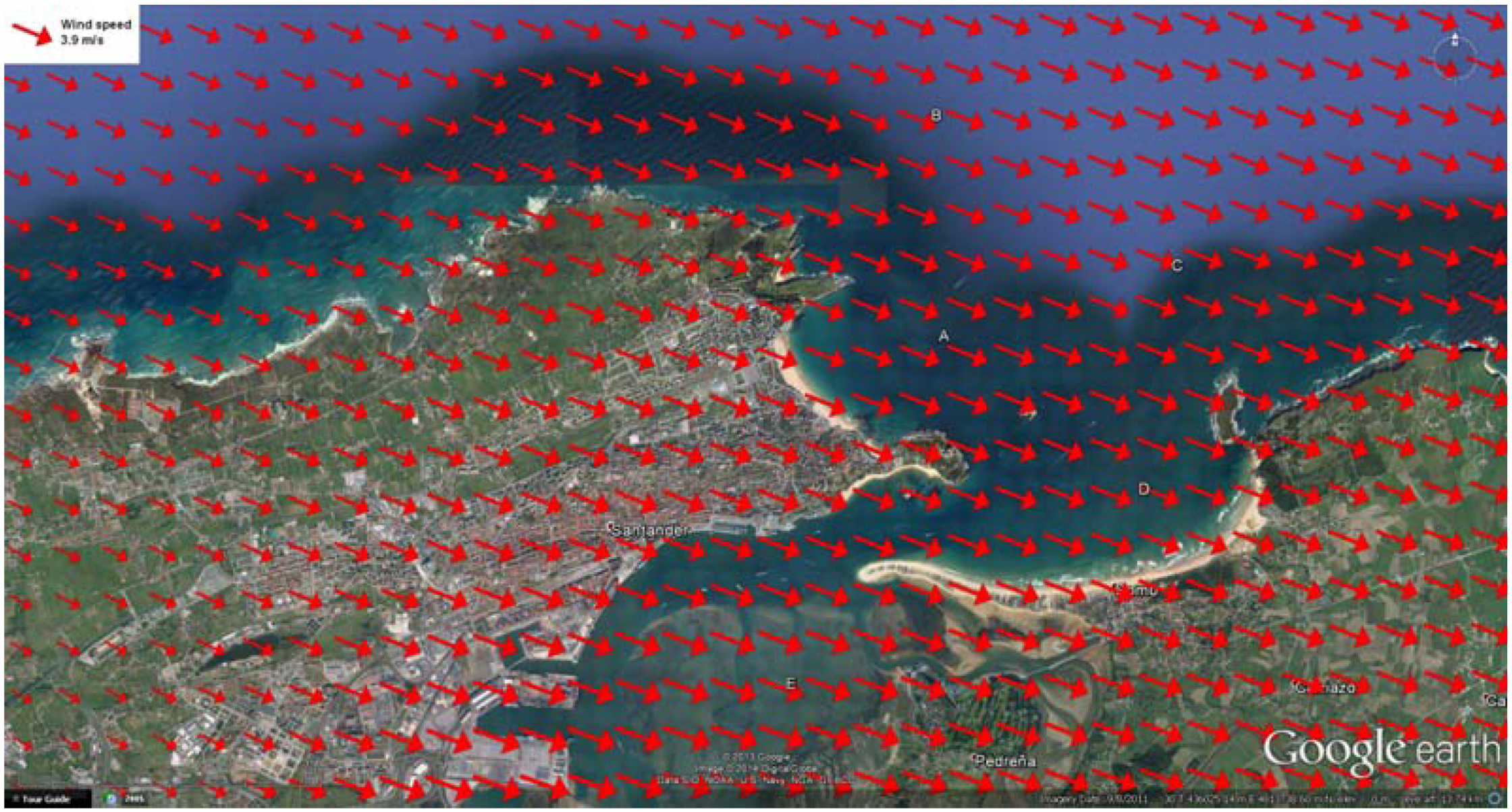
- Wind from W-NW (intensity > 3–4 m/s). Classic and very frequent situation (30%). Characterized by wind rotation to the right till NW and its intensification during the day. The atmospheric pressure slightly increases during the day.
- (4)
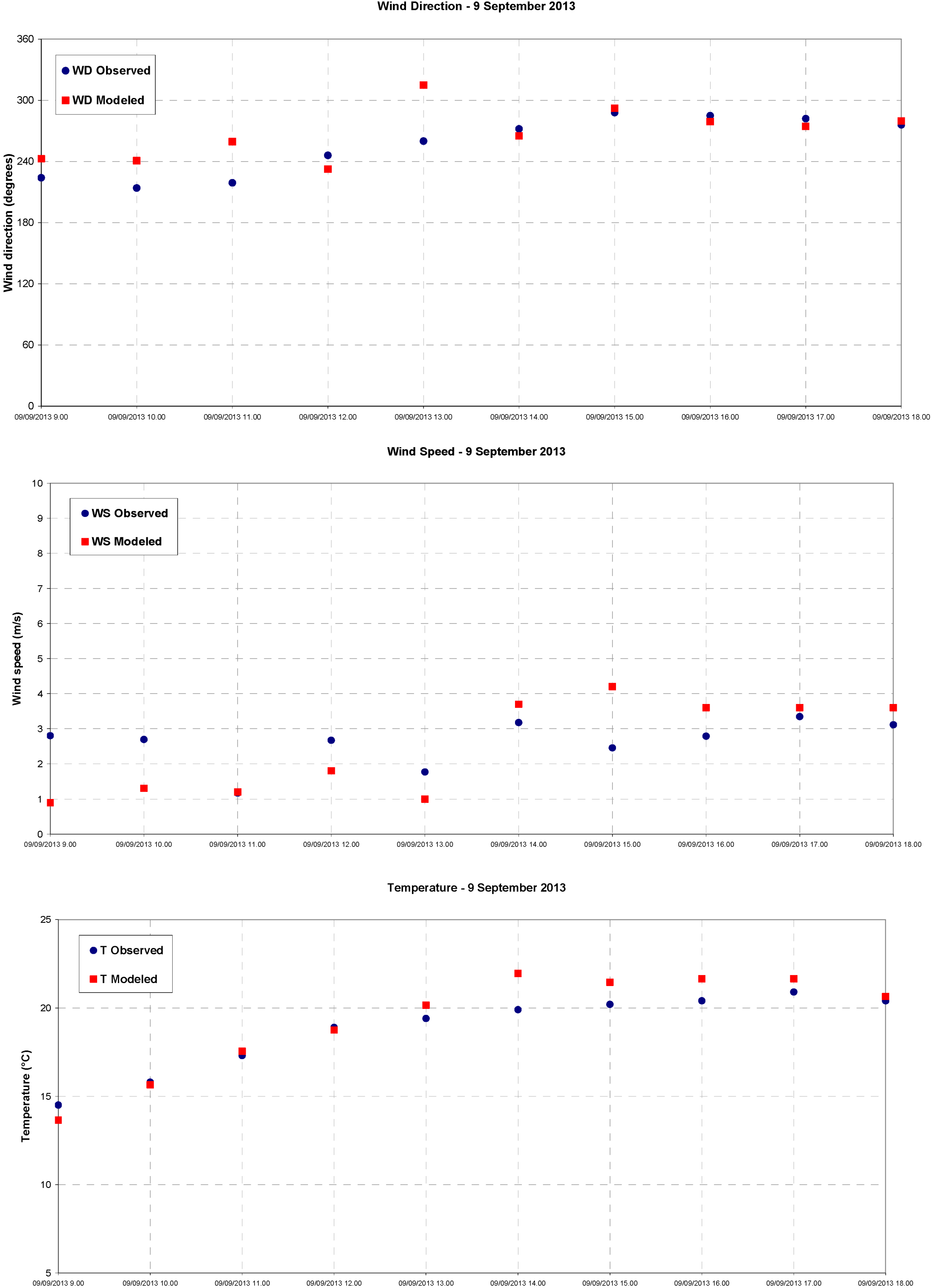
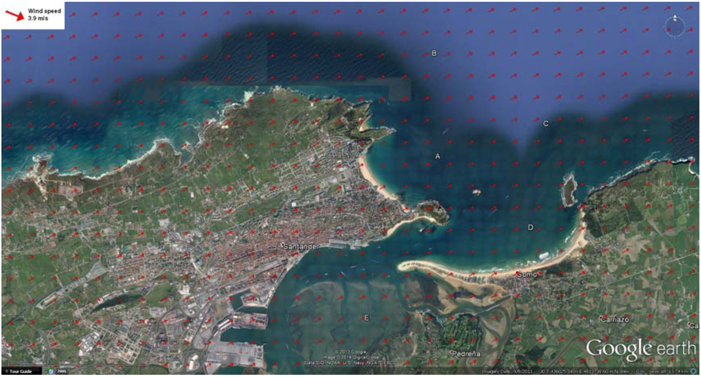
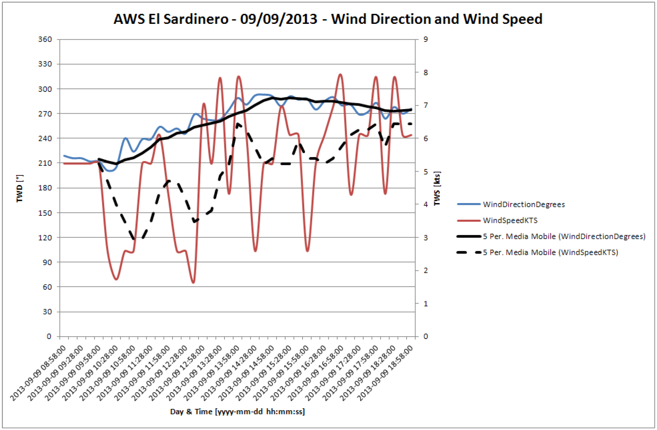
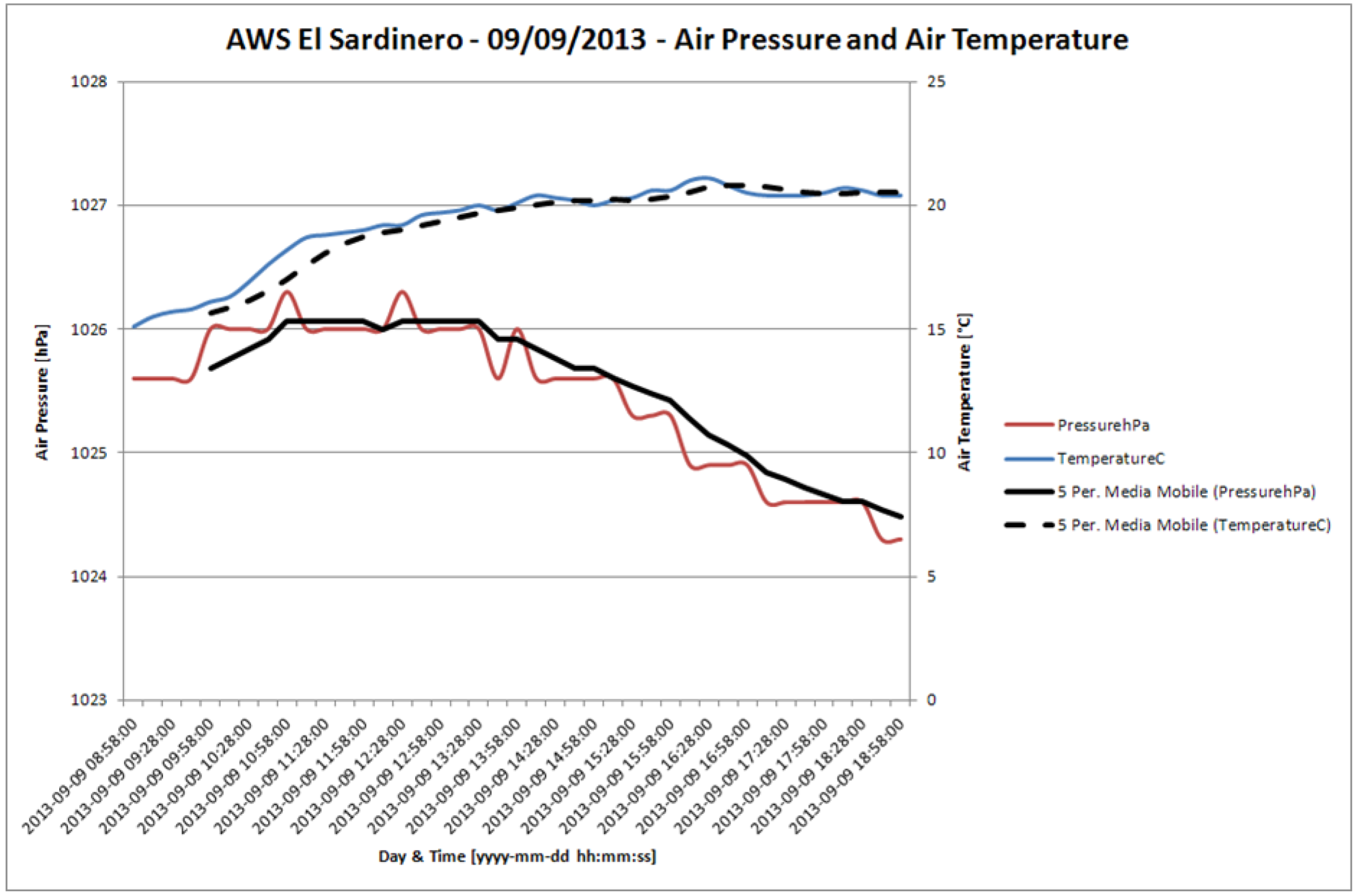
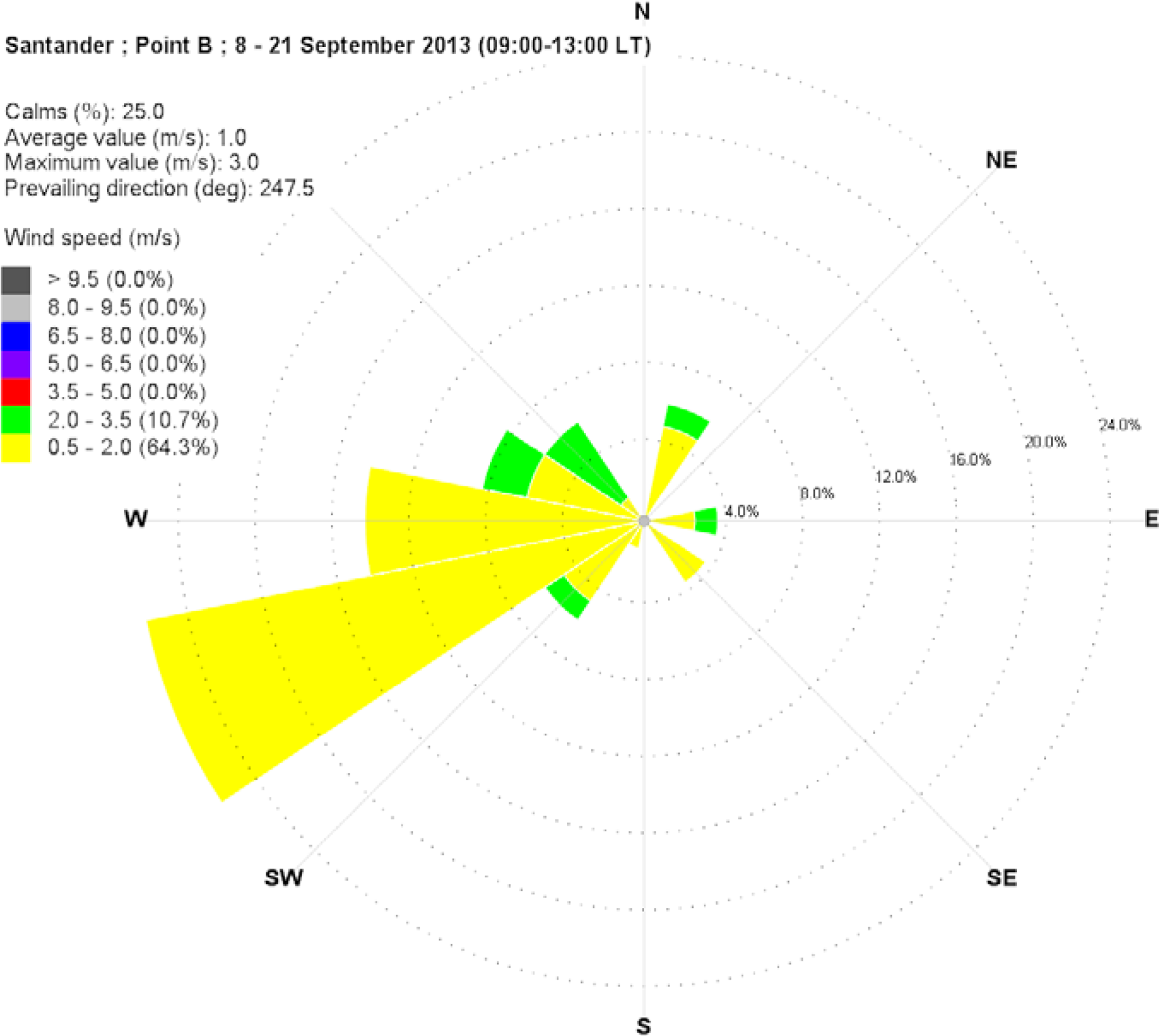
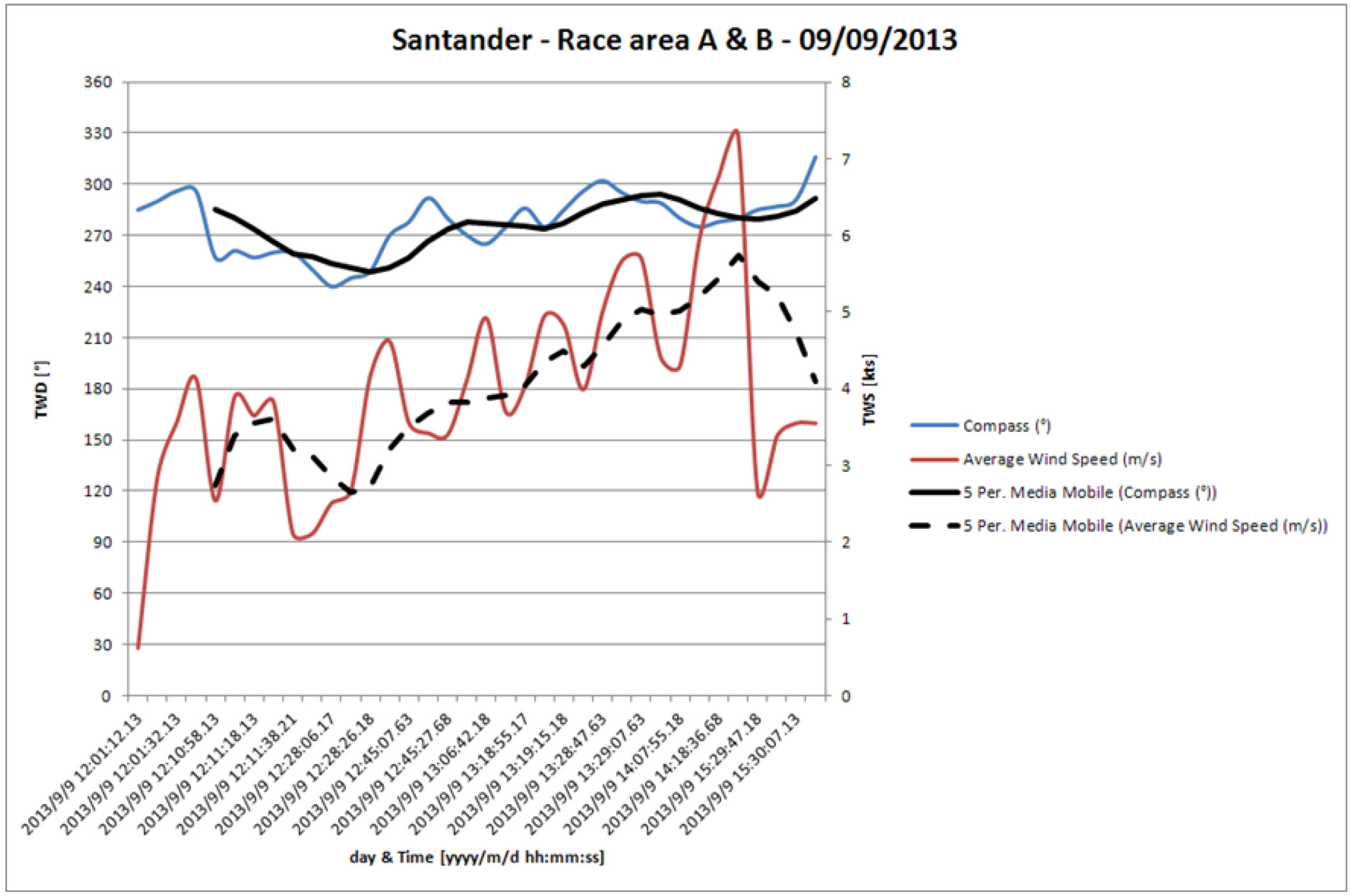
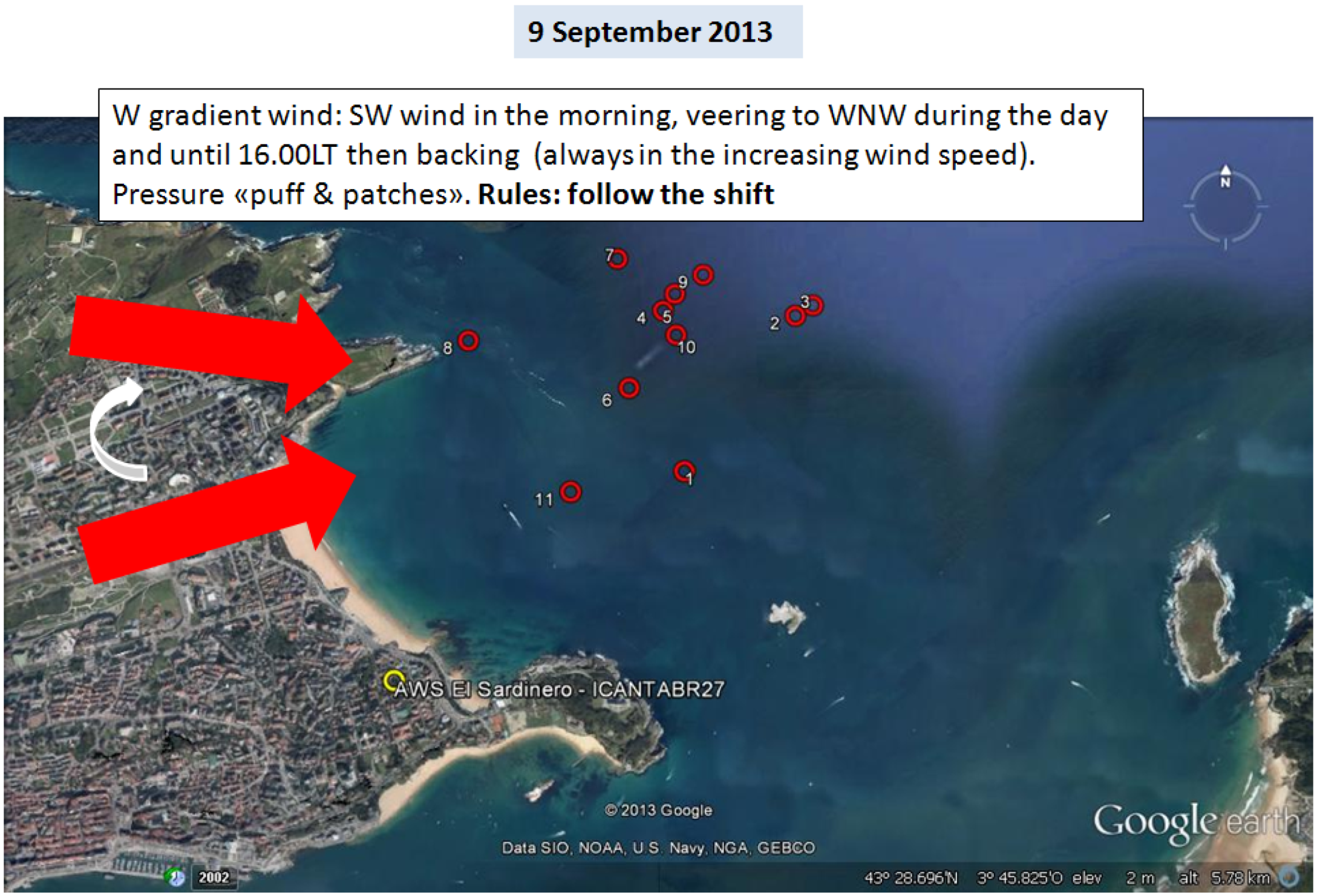
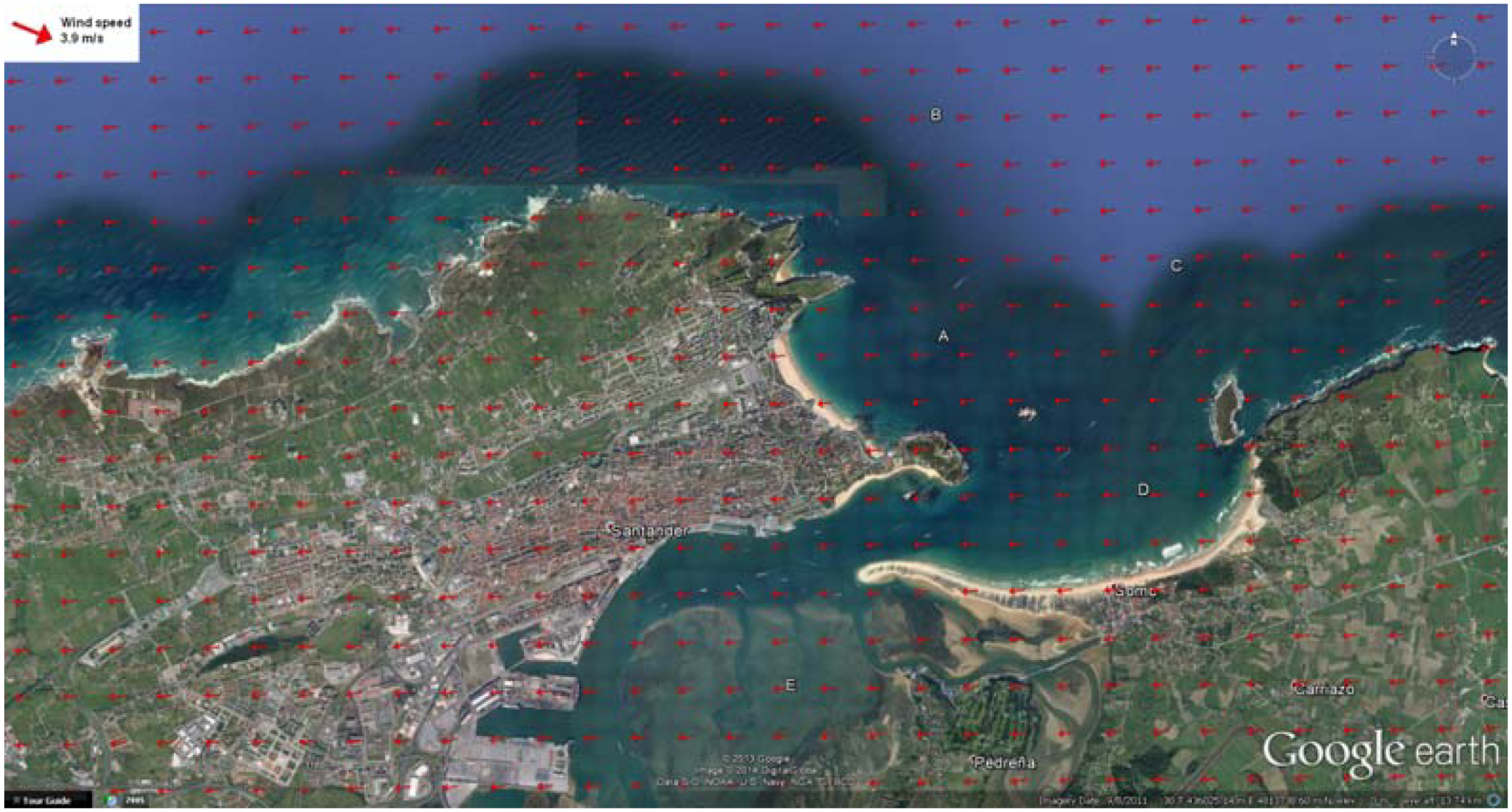
- Wind from W-NW (intensity < 3–4 m/s). This transition situation is observed after the passage of the front and before the establishment of the high pressure conditions. It is quite frequent in the Santander bay (10%). The wind is highly variable in intensity and direction (it could even reach NNW). This is the case of September 9, 2013, which will be analyzed in detail in a following paragraph dedicated to the “Call Book”.
- (5)
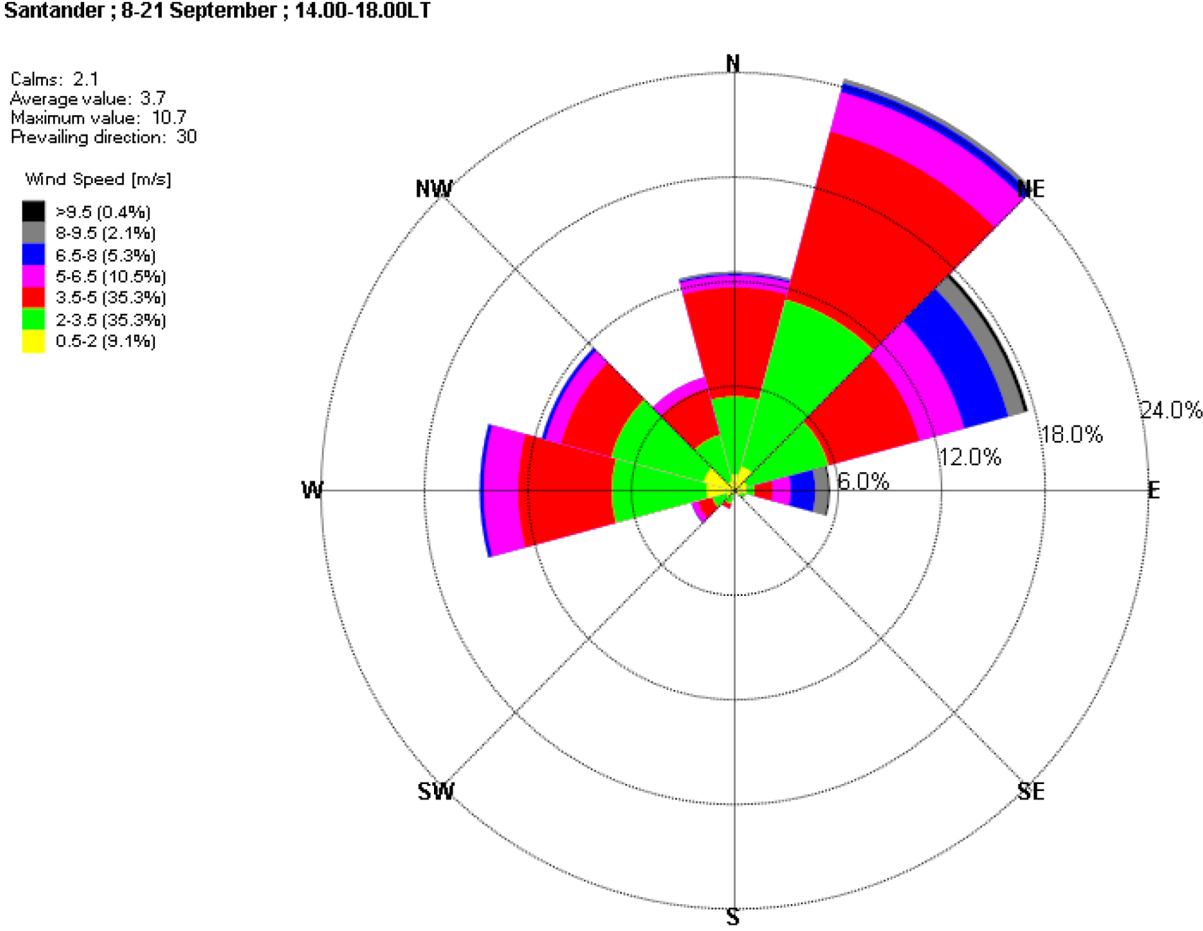
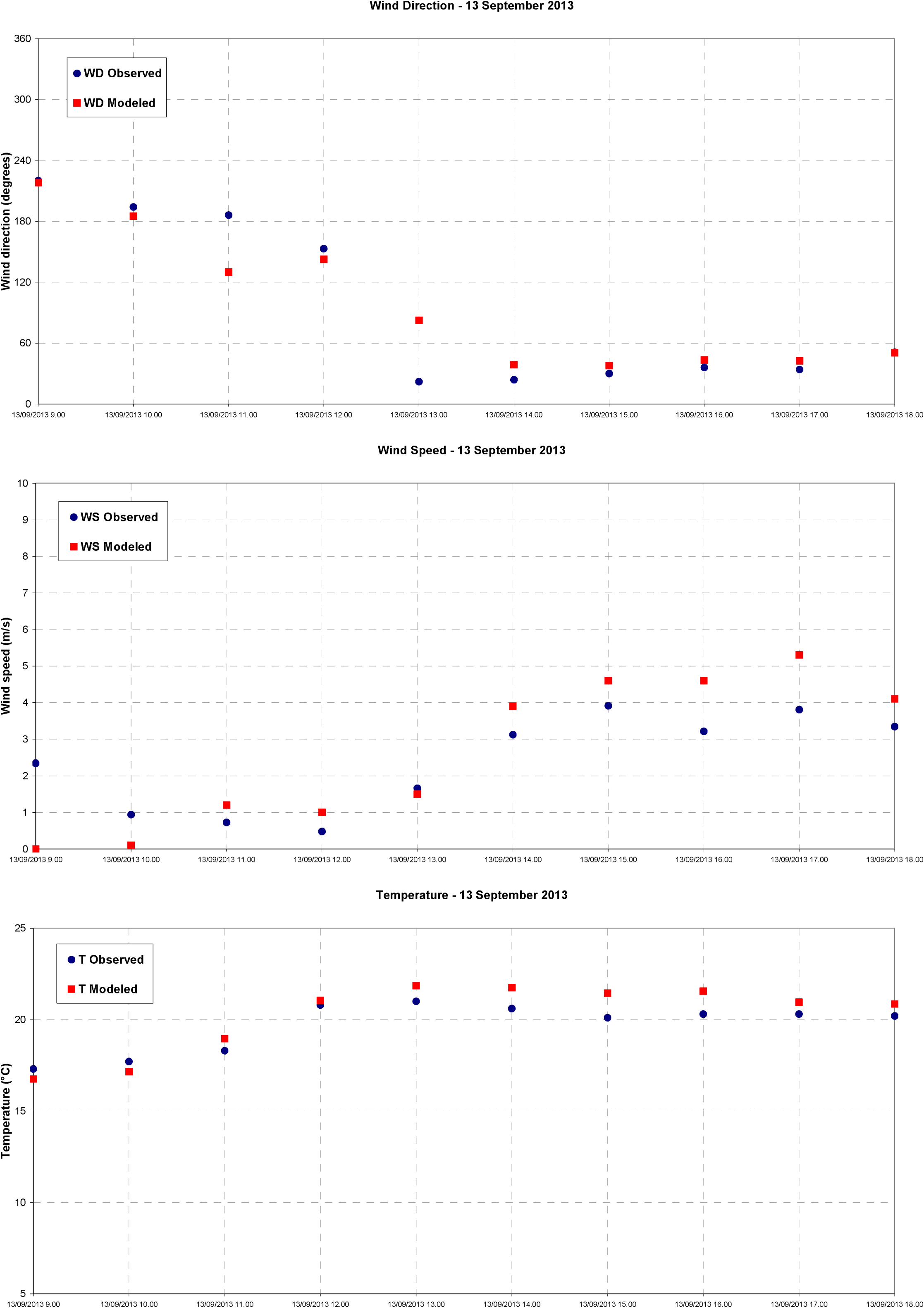
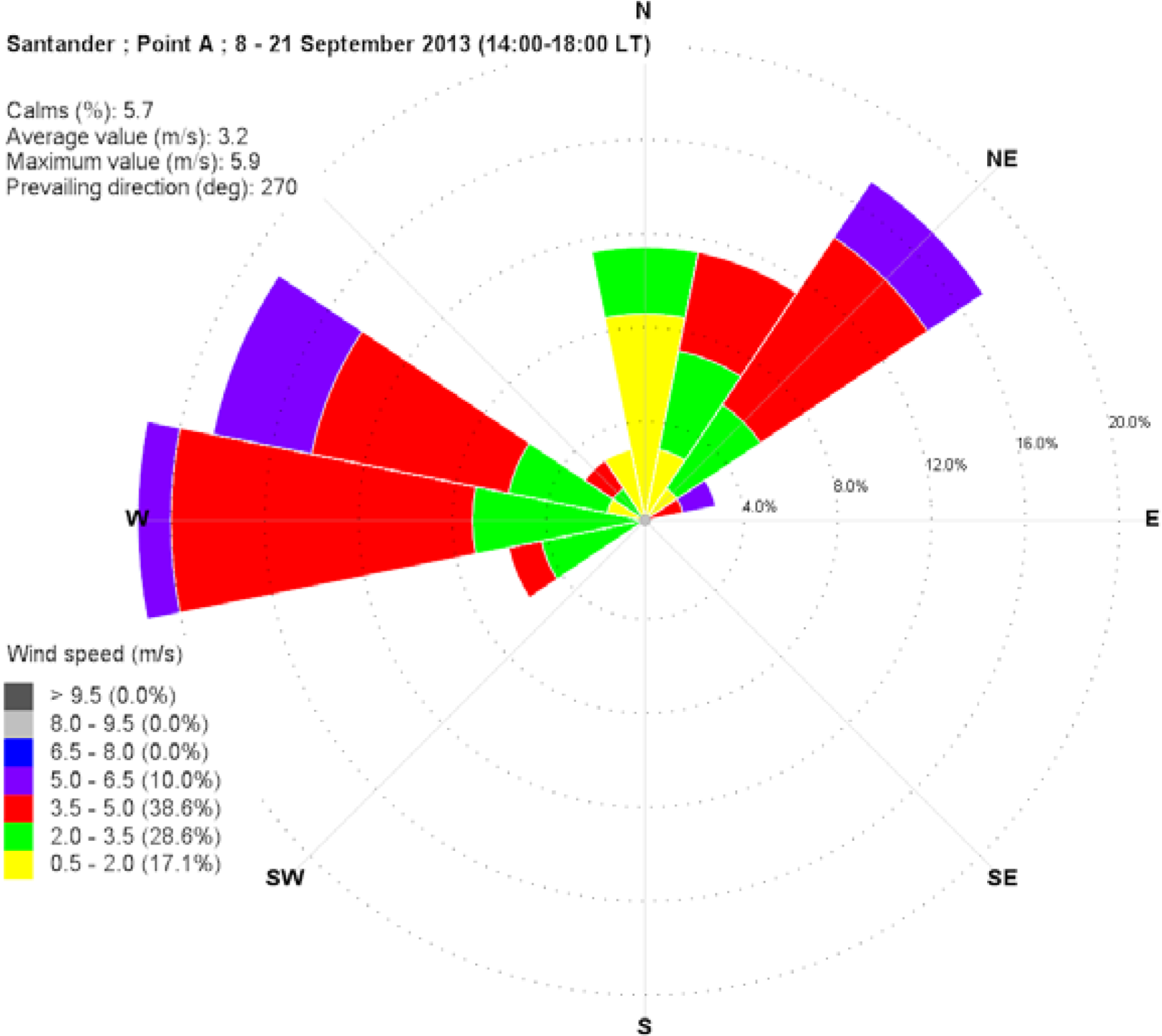
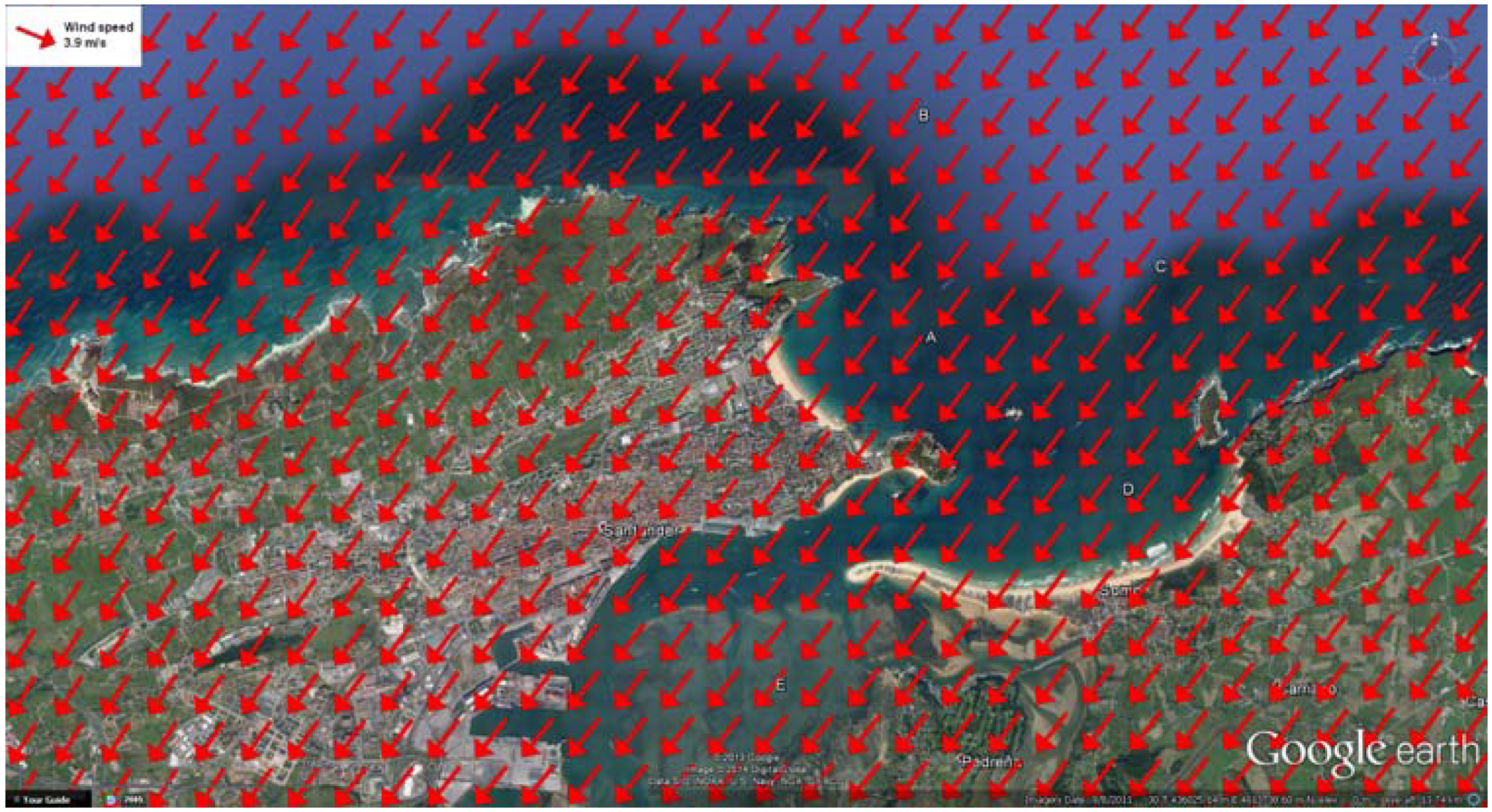
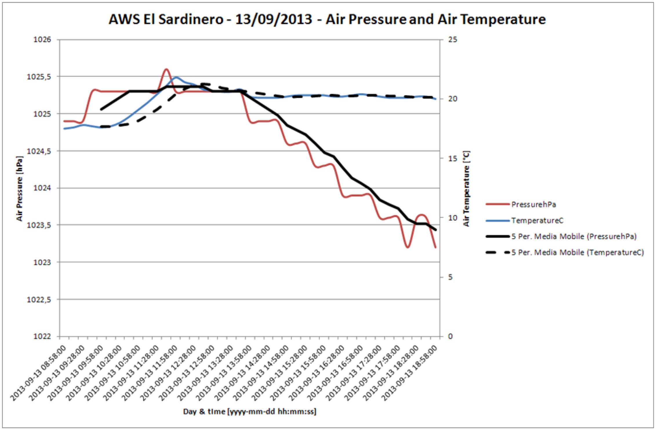
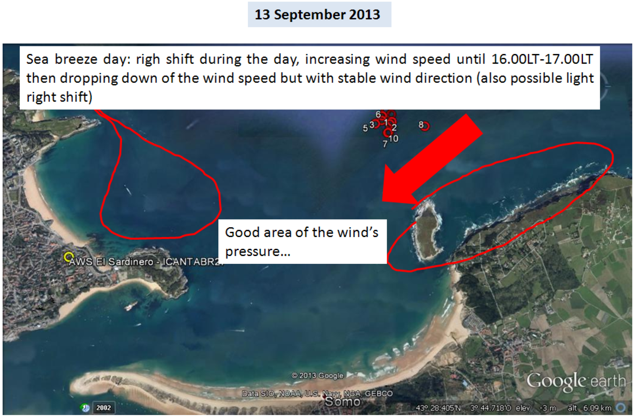
- Wind from NE (sea breeze). Classic sea breeze situation, very frequent in the Santander bay (40%). The atmospheric pressure decreases during the day while the air temperature increases, therefore wind rotates to the right and increases its intensity. This is the case of September 13, 2013, which will be analyzed in detail in a following paragraph dedicated to the “Call Book”.
- (6)
- Wind from ENE (gradient wind). Possible gradient wind without any thermal effect, generated by a depression moving at south of Santander. Quite frequent in the Santander bay (10%), it may generate very intense winds with almost constant direction.


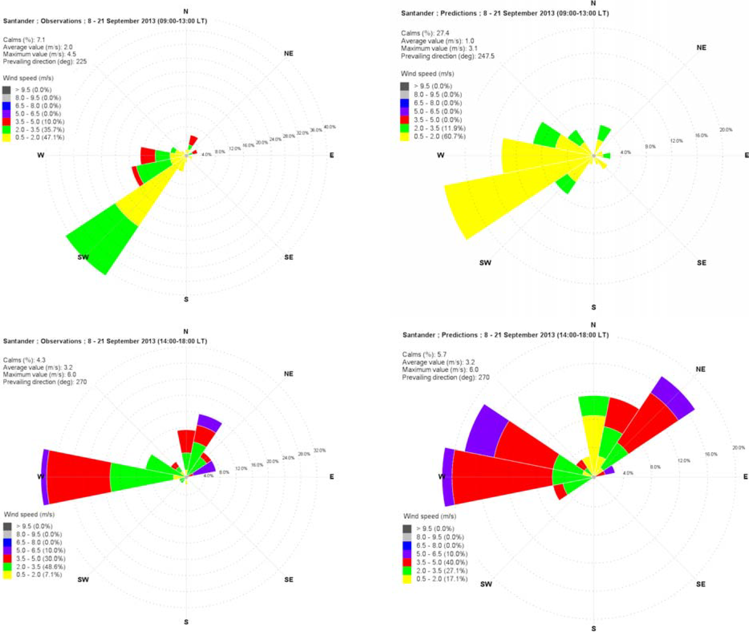
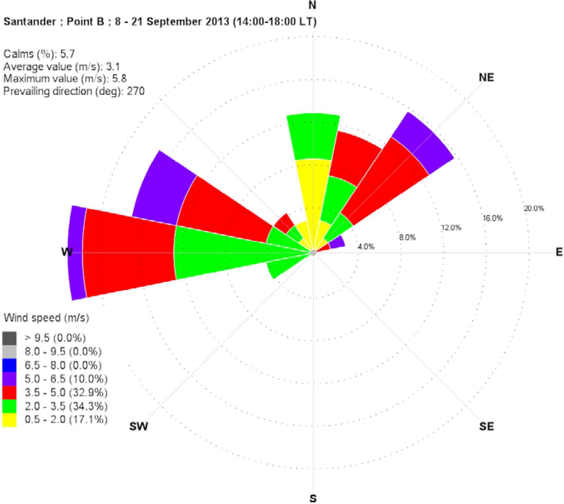
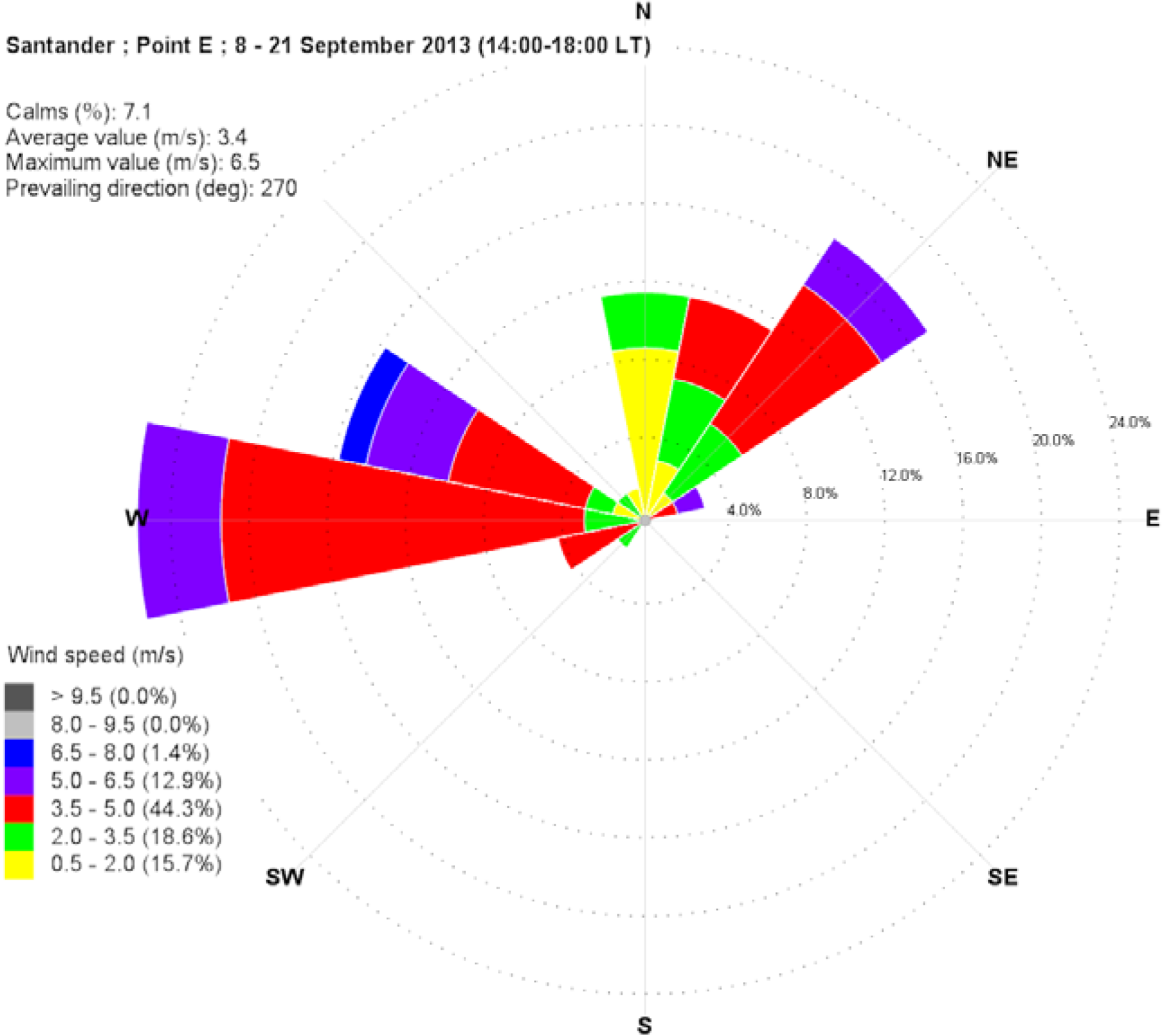
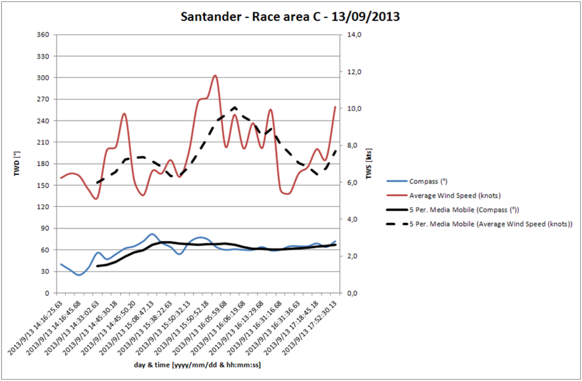
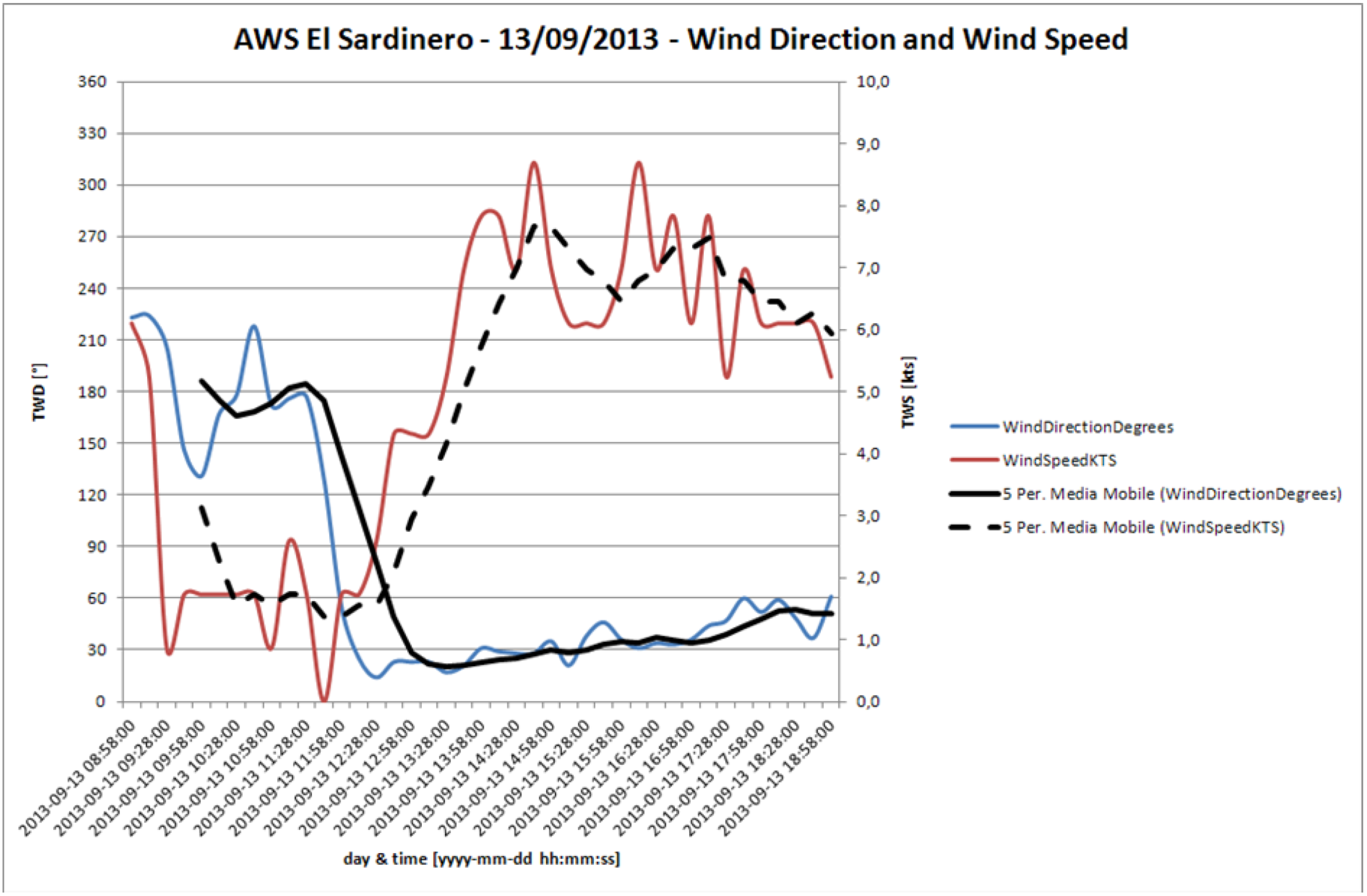
3.2. Comparison against the Observations
- September 9 was characterized as a complex situation, due to the transition between gradient wind and thermal wind;
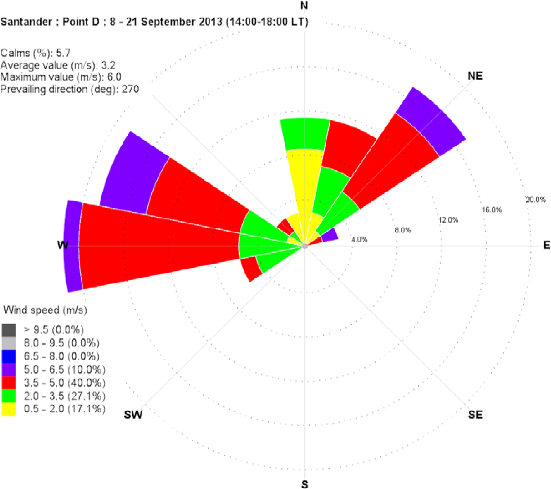
- September 13 was characterized by a pure thermal wind, with counterclockwise wind rotation from south west to north east and decreasing intensity between morning and afternoon, and almost constant wind direction and increased intensity during the afternoon.

| Date | 09–13 | 14–18 | ||||
|---|---|---|---|---|---|---|
| WD | WS | T | WD | WS | T | |
| 08/09/2013 | 18.7 | −5.0 | −3.2 | 9.2 | −44.5 | 2.5 |
| 09/09/2013 | 10.9 | −44.2 | −0.2 | −0.9 | 25.7 | 5.5 |
| 10/09/2013 | −5.8 | −48.4 | −2.6 | 9.1 | −37.2 | −1.0 |
| 11/09/2013 | 9.0 | −42.4 | −0.3 | 2.4 | −1.7 | 0.8 |
| 12/09/2013 | −2.0 | −80.8 | 1.0 | 5.1 | −33.5 | 5.8 |
| 13/09/2013 | −2.2 | −38.3 | 0.7 | 21.9 | 29.4 | 5.0 |
| 14/09/2013 | 7.2 | −34.9 | −1.6 | 2.2 | 2.9 | 2.7 |
| 15/09/2013 | 12.6 | −43.8 | −2.2 | 51.8 | −34.7 | 1.1 |
| 16/09/2013 | 5.2 | −48.6 | −4.8 | −6.6 | −1.9 | −1.0 |
| 17/09/2013 | 9.3 | −37.9 | −1.8 | 1.2 | 20.6 | 1.4 |
| 18/09/2013 | 10.7 | −52.8 | 0.8 | 5.2 | 19.6 | 2.3 |
| 19/09/2013 | 18.7 | −59.2 | −2.7 | −1.2 | 24.8 | 0.9 |
| 20/09/2013 | 6.8 | −37.5 | −0.3 | 12.8 | −10.9 | 1.9 |
| 21/09/2013 | −26.5 | −39.0 | −0.5 | −13.6 | −6.4 | 7.6 |
| Minimum | −26.5 | −80.8 | −4.8 | −13.6 | −44.5 | −1.0 |
| Maximum | 18.7 | −5.0 | 1.0 | 51.8 | 29.4 | 7.6 |
| Average | 5.2 | −43.8 | −1.3 | 7.1 | −3.4 | 2.5 |
| Std. Dev. | 11.6 | 16.3 | 1.7 | 15.4 | 25.8 | 2.6 |
| Date | 09–13 | 14–18 | ||||
|---|---|---|---|---|---|---|
| WD | WS | T | WD | WS | T | |
| 08/09/2013 | 53.5 | 0.7 | 0.7 | 14.0 | 1.5 | 0.6 |
| 09/09/2013 | 30.8 | 1.0 | 0.4 | 5.7 | 0.8 | 1.1 |
| 10/09/2013 | 15.1 | 1.3 | 0.5 | 52.9 | 0.8 | 0.4 |
| 11/09/2013 | 41.1 | 0.6 | 0.4 | 5.3 | 1.1 | 0.3 |
| 12/09/2013 | 19.2 | 1.4 | 0.4 | 14.7 | 1.2 | 1.1 |
| 13/09/2013 | 27.5 | 0.9 | 0.6 | 7.9 | 1.0 | 1.0 |
| 14/09/2013 | 16.8 | 0.8 | 0.3 | 7.3 | 0.4 | 0.6 |
| 15/09/2013 | 34.9 | 0.5 | 0.4 | 13.4 | 0.9 | 0.4 |
| 16/09/2013 | 15.6 | 1.4 | 0.8 | 23.3 | 0.7 | 0.4 |
| 17/09/2013 | 24.2 | 1.2 | 0.5 | 4.4 | 0.8 | 0.3 |
| 18/09/2013 | 26.2 | 1.7 | 0.5 | 14.1 | 0.9 | 0.6 |
| 19/09/2013 | 42.2 | 0.9 | 0.5 | 8.4 | 0.7 | 0.2 |
| 20/09/2013 | 19.1 | 0.7 | 0.3 | 31.7 | 0.6 | 0.4 |
| 21/09/2013 | 51.3 | 0.6 | 1.2 | 10.6 | 0.6 | 1.5 |
| Minimum | 15.1 | 0.5 | 0.3 | 4.4 | 0.4 | 0.2 |
| Maximum | 53.5 | 1.7 | 1.2 | 52.9 | 1.5 | 1.5 |
| Average | 29.8 | 1.0 | 0.5 | 15.3 | 0.8 | 0.6 |
| Std. Dev. | 13.0 | 0.4 | 0.2 | 13.2 | 0.3 | 0.4 |
| Date | 09–13 | 14–18 | ||||
|---|---|---|---|---|---|---|
| WD | WS | T | WD | WS | T | |
| 08/09/2013 | −0.23 | −0.90 | 0.92 | 0.66 | −0.74 | 0.88 |
| 09/09/2013 | −0.12 | 0.23 | 0.99 | 0.75 | −0.79 | −0.20 |
| 10/09/2013 | 0.74 | 0.26 | 0.77 | 0.66 | 1.00 | 0.46 |
| 11/09/2013 | 0.58 | 0.63 | 0.96 | 0.75 | 0.35 | 0.90 |
| 12/09/2013 | 0.68 | −0.55 | 0.99 | 0.74 | 0.67 | −0.73 |
| 13/09/2013 | 0.71 | −0.36 | 0.98 | 0.74 | 0.70 | 0.51 |
| 14/09/2013 | 0.71 | 0.63 | 0.98 | 0.74 | 0.41 | 0.66 |
| 15/09/2013 | 0.68 | 0.82 | 0.98 | 0.72 | 0.78 | 0.85 |
| 16/09/2013 | 0.67 | 0.44 | 0.99 | 0.73 | 0.60 | 0.61 |
| 17/09/2013 | 0.67 | 0.67 | 0.99 | 0.73 | 0.97 | 0.98 |
| 18/09/2013 | 0.66 | 0.63 | 0.95 | 0.73 | 0.87 | 0.03 |
| 19/09/2013 | 0.65 | 0.46 | 0.85 | 0.72 | 0.19 | 0.97 |
| 20/09/2013 | 0.66 | 0.81 | 0.99 | 0.69 | 0.65 | 0.85 |
| 21/09/2013 | 0.59 | 0.98 | 1.00 | 0.69 | 0.40 | 0.52 |
| Minimum | −0.23 | −0.90 | 0.77 | 0.66 | −0.79 | −0.73 |
| Maximum | 0.74 | 0.98 | 1.00 | 0.75 | 1.00 | 0.98 |
| Average | 0.55 | 0.34 | 0.95 | 0.72 | 0.43 | 0.52 |
| Std. Dev. | 0.31 | 0.56 | 0.07 | 0.03 | 0.56 | 0.50 |
3.3. Use of the CALMET Results for Creating the “Call Book”


3.3.1. September 9, 2013


3.3.2. September 13, 2013
4. Conclusions
Acknowledgments
Author Contributions
Conflicts of Interest
References
- Thornes, J.E. The effect of weather on sport. Weather 1977, 32, 258–268. [Google Scholar] [CrossRef]
- Spellman, G. Marathon running an all-weather sport? Weather 1996, 51, 118–125. [Google Scholar] [CrossRef]
- Pezzoli, A.; Moncalero, M.; Boscolo, A.; Cristofori, E.; Giacometto, F.; Gastaldi, S.; Vercelli, G. The meteo-hydrological analysis and the sport performance: which are the connections? The case of the XXI Winter Olympic Games, Vancouver 2010. J. Sports Med. Phys. Fit. 2010, 50, 19–20. [Google Scholar]
- Fleming, P.; Colin, Y.; Dixon, S.; Carré, M. Athlete and coach perception of technology needs for evaluation running performance. Sports Eng. 2010, 13, 1–18. [Google Scholar] [CrossRef]
- Lobozewicz, T. Meteorology in Sport; Sportverlag: Frankfurt, Germany, 1981. [Google Scholar]
- Kay, J.; Vamplew, W. Weather Beaten: Sport in the British Climate; Mainstream Publishing: London, UK, 2002. [Google Scholar]
- Pezzoli, A.; Cristofori, E. Analisi, previsioni e misure meteorologiche applicate agli sport equestri. In Proceedings of the 10th Congress New Findings in Equine Practices, Druento, Italy, 31 October 2008; Centro Internazionale del Cavallo: Druento, Italy, 2008; pp. 38–43. [Google Scholar]
- Olds, T.S.; Norton, K.I.; Lowe, E.L.; Olive, S.; Reay, F.; Ly, S. Modeling road-cycling performance. J. Appl. Physiol. 1995, 78, 1596–1611. [Google Scholar] [PubMed]
- Peiffer, J.J.; Abbiss, C.R. Influence of environmental temperature on 40 km cycling time-trial performance. Int. J. Sports Physiol. Perform. 2011, 6, 208–220. [Google Scholar] [PubMed]
- Pezzoli, A.; Baldacci, A.; Cama, A.; Faina, M.; Dalla Vedova, D.; Besi, M.; Vercelli, G.; Boscolo, A.; Moncalero, M.; Cristofori, E.; et al. Wind-wave interactions in enclosed basins: The impact on the sport of rowing. In Sport Physics; Clanet, C., Ed.; Ecole Polytechnique de Paris: Paris, France, 2013; pp. 139–151. [Google Scholar]
- Pezzoli, A.; Cristofori, E.; Moncalero, M.; Giacometto, F.; Boscolo, A. Effect of the environment on the sport performance. In Proceeding of the International Congress on Sports Science Research and Technology Support, Vilamoura, Portugal, 20–22 September 2013; SCITEPRESS: Portugal, 2013; pp. 167–170. [Google Scholar]
- Buchheit, M.; Voss, S.C.; Nybo, L.; Mohr, M.; Racinais, S. Physiological and performance adaptations to an in-season soccer camp in the heat: association with heart rate and heart rate variability. Scand. J. Med. Sci. Sports 2011, 21, e477–e485. [Google Scholar] [CrossRef] [PubMed]
- Opatkiewicz, A.; Williams, T.; Walters, C. The effects of temperature, travel and time off on Major League soccer team performance. In Proceeding of the World Congress of Performance Analysis of Sport IX, Worcester, UK, 25–28 July 2012; University of Worcester: Worcester, UK, 2012. [Google Scholar]
- Brocherie, F.; Girard, O.; Farooq, A.; Millet, G.P. Climatic influence on home advantage in Gulf Region Football. In Proceeding of the International Congress on Sports Science Research and Technology Support, Vilamoura, Portugal, 20–22 September 2013; SCITEPRESS: Portugal, 2013. [Google Scholar]
- Pezzoli, A.; Cristofori, E.; Gozzini, B.; Marchisio, M.; Padoan, J. Analysis of the thermal comfort in cycling athletes. Procedia Eng. 2012, 34, 433–438. [Google Scholar] [CrossRef]
- Vihma, T. Effects of weather on the performance of marathon runners. Int. J. Biometeorol. 2010, 54, 297–306. [Google Scholar] [CrossRef] [PubMed]
- El Helou, N.; Tafflet, M.; Berthelot, G.; Tolaini, J.; Marc, A.; Guillame, M.; Hausswirth, C.; Toussaint, J.F. Impact of environmental parameters on marathon running performance. PLoS One 2012, 7, e37407. [Google Scholar] [CrossRef] [PubMed]
- Gonzales, B.R.; Hagin, V.; Guillot, R.; Placet, V.; Groslambert, A. Effect of polyester jerseys on psycho-physiological responses during exercise in a hot and moist environment. J. Strengh Cond. Res. 2011, 12, 3432–3438. [Google Scholar] [CrossRef]
- Davis, J.K.; Bishop, P.A. Impact of clothing on exercise in the heat. Sports Med. 2013, 695–706. [Google Scholar] [CrossRef]
- Colonna, M.; Moncalero, M.; Nicotra, M.; Pezzoli, A.; Fabbri, E.; Bortolan, L.; Pellegrini, B.; Schena, F. Thermal behaviour of ski-boot liners: effect of materials on thermal comfort in real and simulated skiing conditions. Procedia Eng. 2014, 72, 386–391. [Google Scholar] [CrossRef]
- Houghton, D. Wind for sailors. Weather 1993, 48, 414–419. [Google Scholar] [CrossRef]
- Del Prete, R.; Pezzoli, A.; Pezzoli, G. Current methods for meteorological and marine forecasting for the assistance of navigation and shipping operation. J. Navig. 1999, 1, 104–118. [Google Scholar] [CrossRef]
- Pezzoli, A.; Franza, M. Safety of navigation, ballast water and meteomarine forecast: Analysis and reliability. J. Navig. 2000, 3, 541–550. [Google Scholar] [CrossRef]
- Pezzoli, A.; Cristofori, E.; Vercelli, G.; Gambarino, C. La comunicazione nello sport della vela: Area di conoscenza, processo o prodotto di progetto? Il caso studio di un Weather Team in un Challenger di Coppa America. Il Giornale Italiano di Psicologia dello Sport 2011, 10, 20–27. [Google Scholar]
- Bethwaite, F. High Performance Sailing, Faster Racing Techniques, 2nd ed.; Adlard Coles Nautical: London, UK, 2011. [Google Scholar]
- Pezzoli, A. A dynamic approach to hydrology problems: a study of disastrous pluviometric events through weather type analysis. Atti. dell’Accademia delle Scienze di Torino 1995, 129, 47–59. [Google Scholar]
- Enke, W.; Spekat, A. Downscaling climate model outputs into local and regional weather elements by classification and regression. Clim. Res. 1997, 8, 195–207. [Google Scholar] [CrossRef]
- Enke, W.; Deutschlander, T.; Schneider, F.; Kuchler, W. Results of five regional climate studies applying a weather pattern based downscaling method to ECHAM4 climate simulation. Meteorol. Z. 2005, 14, 247–257. [Google Scholar] [CrossRef]
- Scire, J.S.; Robe, F.R.; Fernau, M.E.; Yamartino, R.J. A User’s Guide for the CALMET Meteorological Model, 5th ed.; Earth Tech. Inc.: Concord, MA, USA, 2000. [Google Scholar]
- Scire, J.S.; Strimaitis, D.G.; Yamartino, R.J. A User’s Guide for the CALPUFF Dispersion Model, 5th ed.; Earth Tech. Inc.: Concord, MA, USA, 2000. [Google Scholar]
- Enviroware. Available online: http://www.enviroware.com/portfolio/windrose-pro3/ (accessed on 18 February 2014).
- JDC Instruments. Available online: http://www.jdc.ch/en/scientific-line/geos/ (accessed on 6 June 2014).
- Garmin. Available online: http://sites.garmin.com/forerunner910xt/?lang=en&country=US (accessed on 6 June 2014).
- Mosca, S.A.; Graziani, G.; Klug, W.; Bellasio, R.; Bianconi, R. A statistical methodology for the evaluation of long-range dispersion models: An application to the ETEX exercise. Atmos. Environ. 1998, 24, 4307–4324. [Google Scholar] [CrossRef]
- Pezzoli, A.; Tedeschi, G.; Resch, F. Numerical simulation of strong wind situations near the French Mediterranean Coast: Comparison with FETCH data. J. Appl. Meteorol. 2004, 43, 997–1015. [Google Scholar] [CrossRef]
- Wilks, D.S. Statistical Methods in the Atmospheric Sciences; Academic Press: San Diego, CA, USA, 1995. [Google Scholar]
- Houghton, D.; Campbell, F. Wind Strategy, 3rd ed.; John Wiley & Sons Inc.: London, UK, 2006. [Google Scholar]
- Pezzoli, A. Observation and analysis of Etesian wind storms in the Saroniko Gulf. Adv. Geosci. 2005, 2, 187–194. [Google Scholar] [CrossRef]
- Cohen, J. Statistical Power Analysis for the Behavioral Sciences, 2nd ed.; Lawrence Erlbaum: Hillsdale, NJ, USA, 1988. [Google Scholar]
- Rosenthal, J.A. Qualitative descriptors of strength of association and effect size. J. Soc. Serv. Res. 1996, 21, 37–59. [Google Scholar] [CrossRef]
© 2014 by the authors; licensee MDPI, Basel, Switzerland. This article is an open access article distributed under the terms and conditions of the Creative Commons Attribution license (http://creativecommons.org/licenses/by/4.0/).
Share and Cite
Pezzoli, A.; Bellasio, R. Analysis of Wind Data for Sports Performance Design: A Case Study for Sailing Sports. Sports 2014, 2, 99-130. https://doi.org/10.3390/sports2040099
Pezzoli A, Bellasio R. Analysis of Wind Data for Sports Performance Design: A Case Study for Sailing Sports. Sports. 2014; 2(4):99-130. https://doi.org/10.3390/sports2040099
Chicago/Turabian StylePezzoli, Alessandro, and Roberto Bellasio. 2014. "Analysis of Wind Data for Sports Performance Design: A Case Study for Sailing Sports" Sports 2, no. 4: 99-130. https://doi.org/10.3390/sports2040099
APA StylePezzoli, A., & Bellasio, R. (2014). Analysis of Wind Data for Sports Performance Design: A Case Study for Sailing Sports. Sports, 2(4), 99-130. https://doi.org/10.3390/sports2040099