Figure 1.
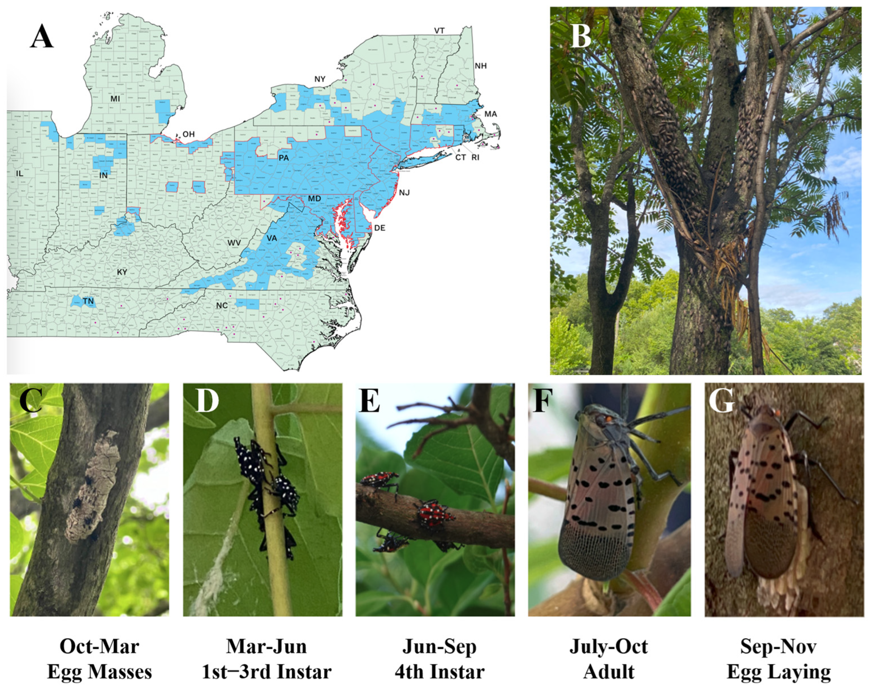
(A) SLF distribution map across the eastern U.S. (B) SLF infestation on a TOH along the Landsdown Trail, Clinton, NJ, USA. (C–G) SLF life cycle. Map in (A) courtesy of Cornell University College of Agriculture and Life Sciences (CALS).
Figure 1.
(A) SLF distribution map across the eastern U.S. (B) SLF infestation on a TOH along the Landsdown Trail, Clinton, NJ, USA. (C–G) SLF life cycle. Map in (A) courtesy of Cornell University College of Agriculture and Life Sciences (CALS).
Figure 2.
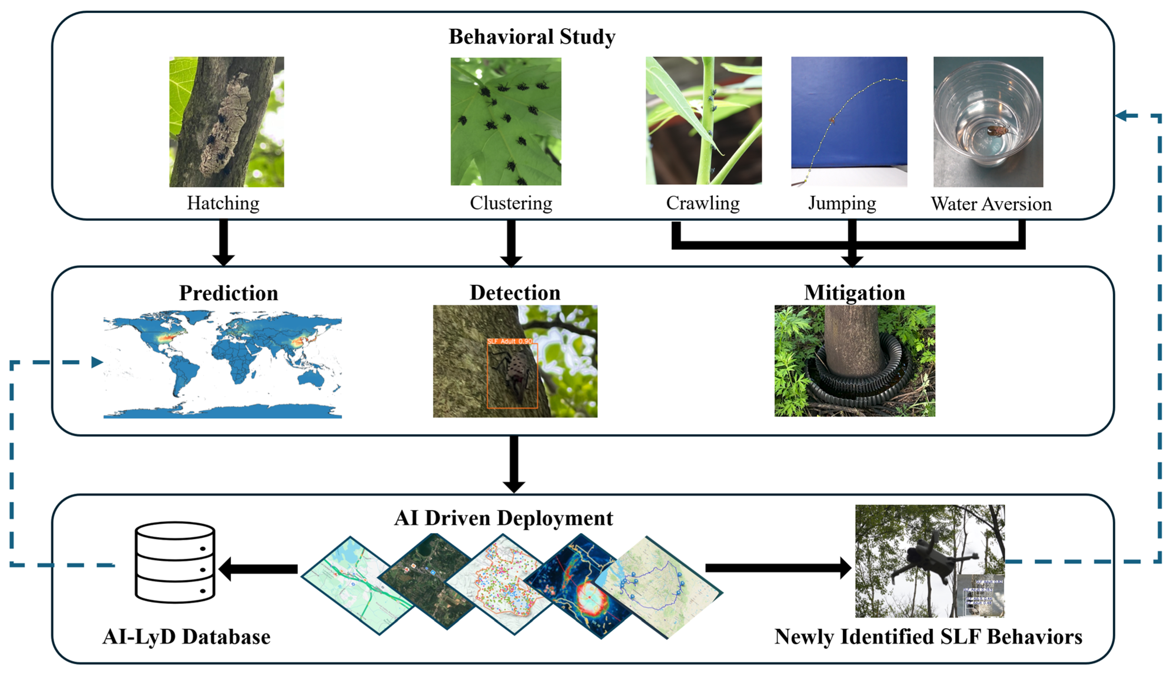
AI-LyD’s system-level architecture for understanding and reducing SLF populations. The framework consists of three phases, each with distinct objectives and research focus.
Figure 2.
AI-LyD’s system-level architecture for understanding and reducing SLF populations. The framework consists of three phases, each with distinct objectives and research focus.
Figure 3.
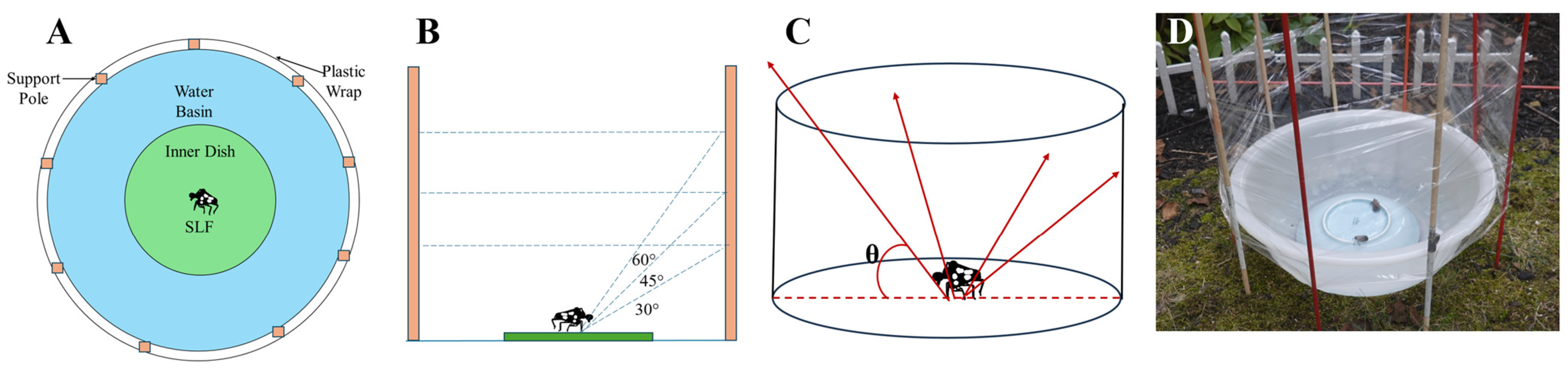
Experimental setup for SLF jumping experiments: (A) Bird’s-eye view diagram of testing environment; (B) Side view; (C) Three-dimensional schematic, with red arrows indicating different possible jumping trajectories; (D) Picture of the actual setup.
Figure 3.
Experimental setup for SLF jumping experiments: (A) Bird’s-eye view diagram of testing environment; (B) Side view; (C) Three-dimensional schematic, with red arrows indicating different possible jumping trajectories; (D) Picture of the actual setup.
Figure 4.
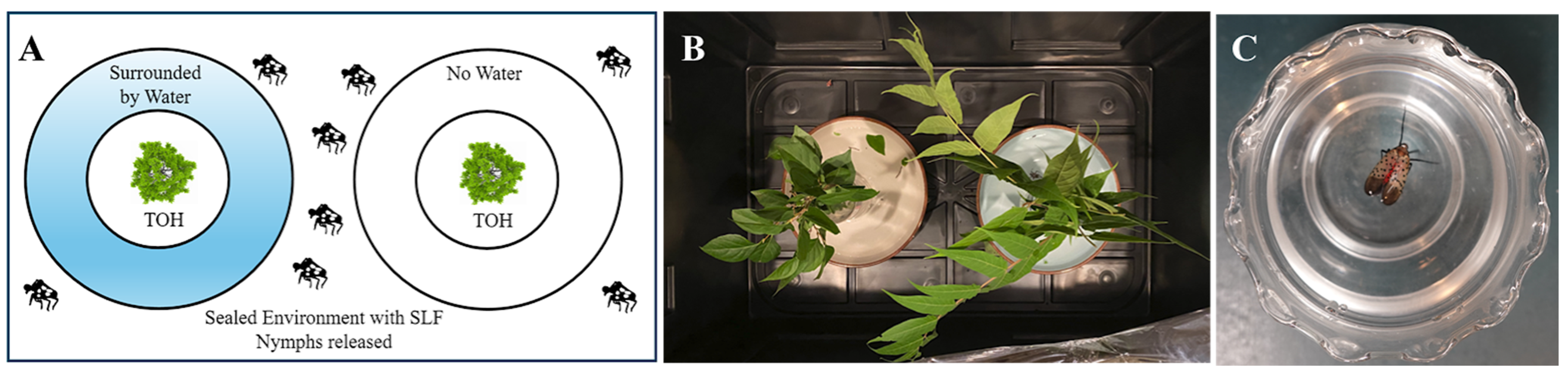
Experimental setup for SLF hydrophobicity tests. (A) Experimental Setup for Testing SLF Hydrophobicity. (B) TOH branches placed in a sealed environment: one with a water-filled moat and the other with an empty moat. (C) SLF survival assay in different solutions: water, 5% ECOS dish detergent, 5% DAWN dish detergent.
Figure 4.
Experimental setup for SLF hydrophobicity tests. (A) Experimental Setup for Testing SLF Hydrophobicity. (B) TOH branches placed in a sealed environment: one with a water-filled moat and the other with an empty moat. (C) SLF survival assay in different solutions: water, 5% ECOS dish detergent, 5% DAWN dish detergent.
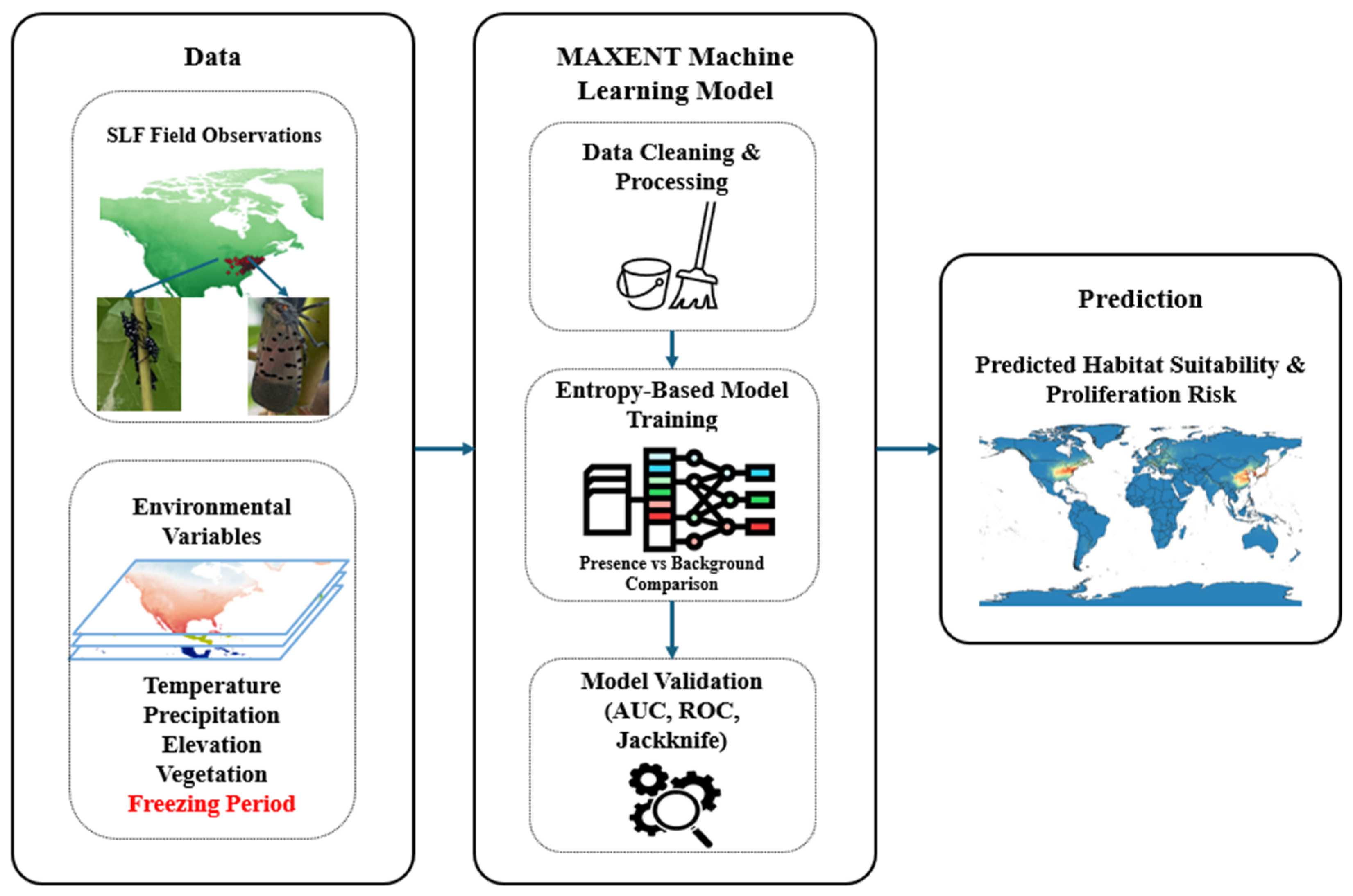
Figure 5.
MAXENT data architecture. Environmental layers and occurrence point data are prepared, trained, and validated through statistical analysis (ex. AUC test).
Figure 5.
MAXENT data architecture. Environmental layers and occurrence point data are prepared, trained, and validated through statistical analysis (ex. AUC test).
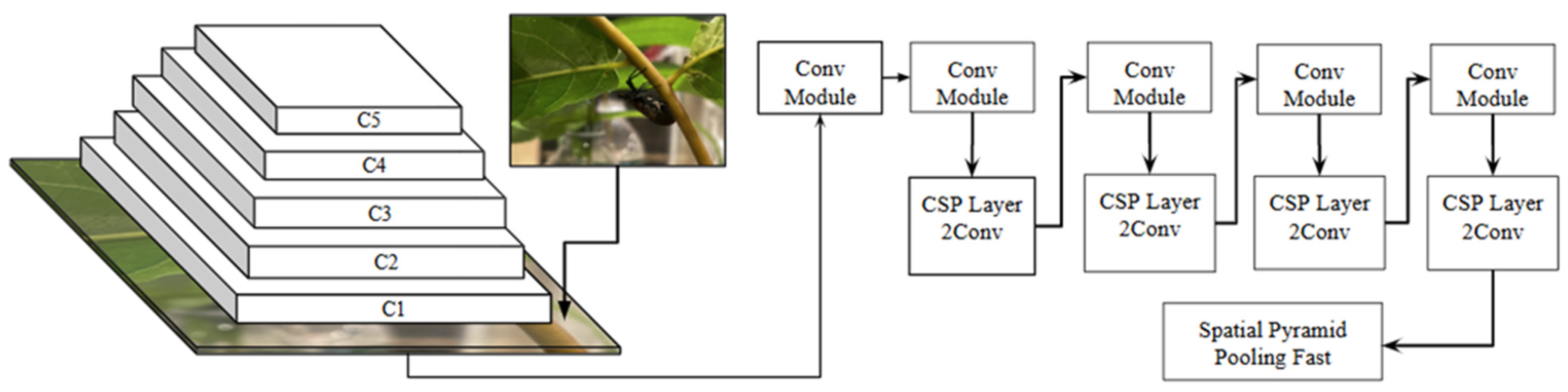
Figure 6.
YOLO-v11 data architecture of the backbone. The convolutional layers are responsible for extracting features from the input image, which will be fed into the neck and head of the YOLO model.
Figure 6.
YOLO-v11 data architecture of the backbone. The convolutional layers are responsible for extracting features from the input image, which will be fed into the neck and head of the YOLO model.
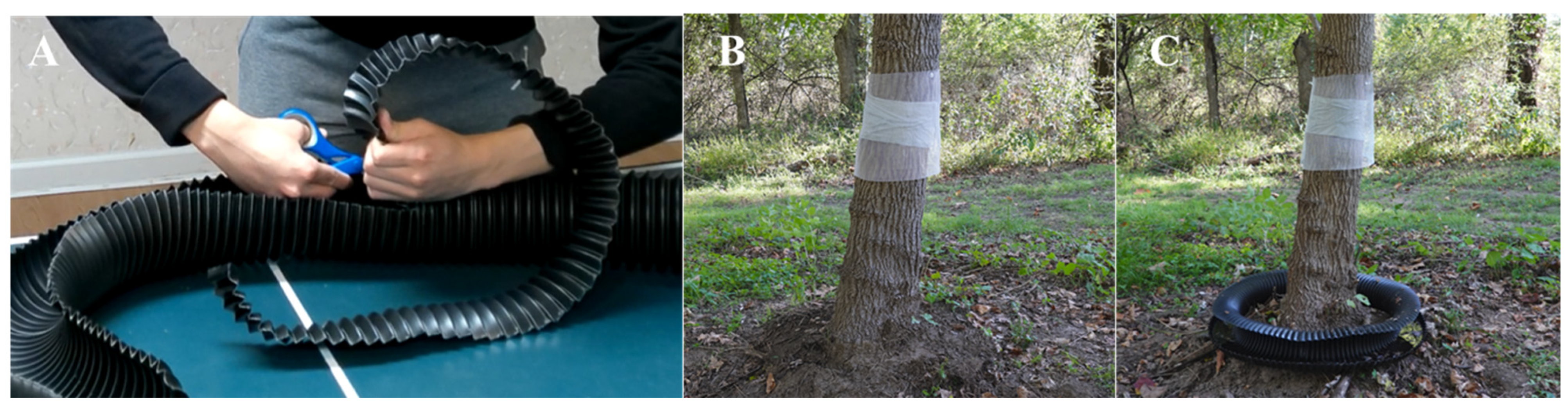
Figure 7.
(A) Fabrication of Aquabex from a 4-inch drain pipe (B) A black walnut tree (Landstown Trail, Clinton, NJ, USA) with sticky band and protection screen without Aquabex; (C) the same black walnut tree with Aquabex.
Figure 7.
(A) Fabrication of Aquabex from a 4-inch drain pipe (B) A black walnut tree (Landstown Trail, Clinton, NJ, USA) with sticky band and protection screen without Aquabex; (C) the same black walnut tree with Aquabex.
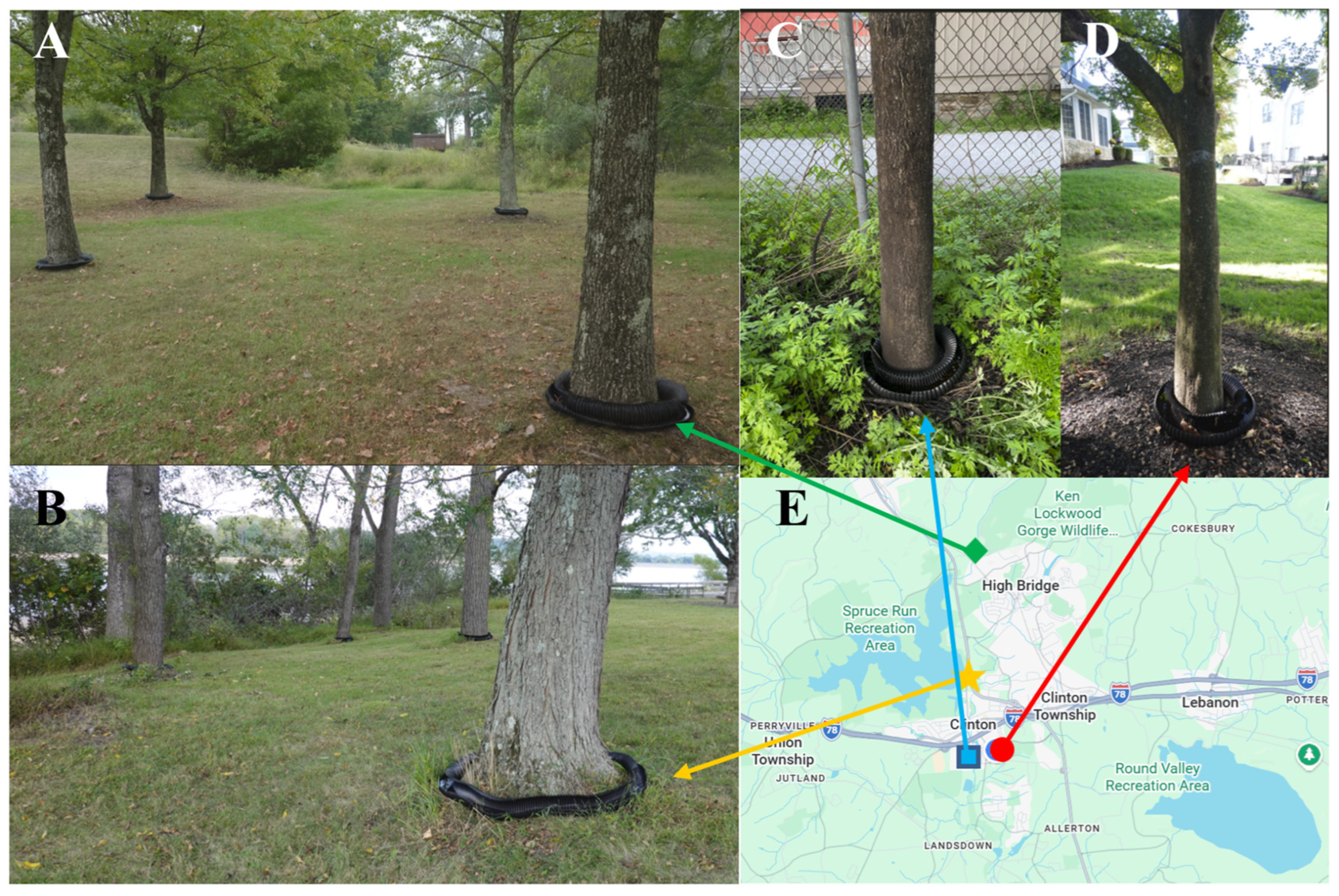
Figure 8.
Aquabex deployment: (A) Site 1, Aquabex deployed at a private property in High Bridge, NJ, USA; (B) Site 2, Aquabex deployed near Spruce Run Reserve in Annandale, NJ, USA; (C) Site 3, Aquabex deployed on a TOH near Landsdown Trail; and (D) Site 4, Aquabex deployed at a private property in Clinton, NJ, USA. (E) Geographical map showing the test site locations with various icons.
Figure 8.
Aquabex deployment: (A) Site 1, Aquabex deployed at a private property in High Bridge, NJ, USA; (B) Site 2, Aquabex deployed near Spruce Run Reserve in Annandale, NJ, USA; (C) Site 3, Aquabex deployed on a TOH near Landsdown Trail; and (D) Site 4, Aquabex deployed at a private property in Clinton, NJ, USA. (E) Geographical map showing the test site locations with various icons.
Figure 9.
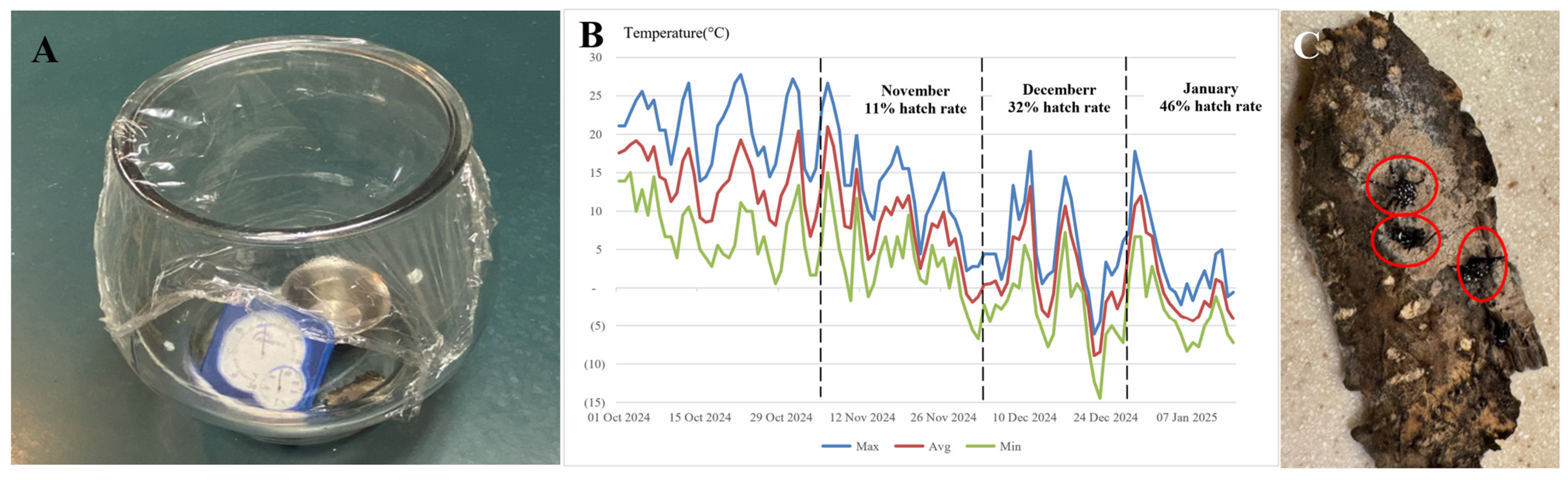
(A) SLF hatching environment under constant temperature of 25 °C and humidity of 70% (B) Daily temperature data sourced from National Centers for Environmental Information for Clinton, New Jersey, where the SLF eggs were collected. (C) Red circles indicate newly hatched SLF nymphs.
Figure 9.
(A) SLF hatching environment under constant temperature of 25 °C and humidity of 70% (B) Daily temperature data sourced from National Centers for Environmental Information for Clinton, New Jersey, where the SLF eggs were collected. (C) Red circles indicate newly hatched SLF nymphs.
Figure 10.
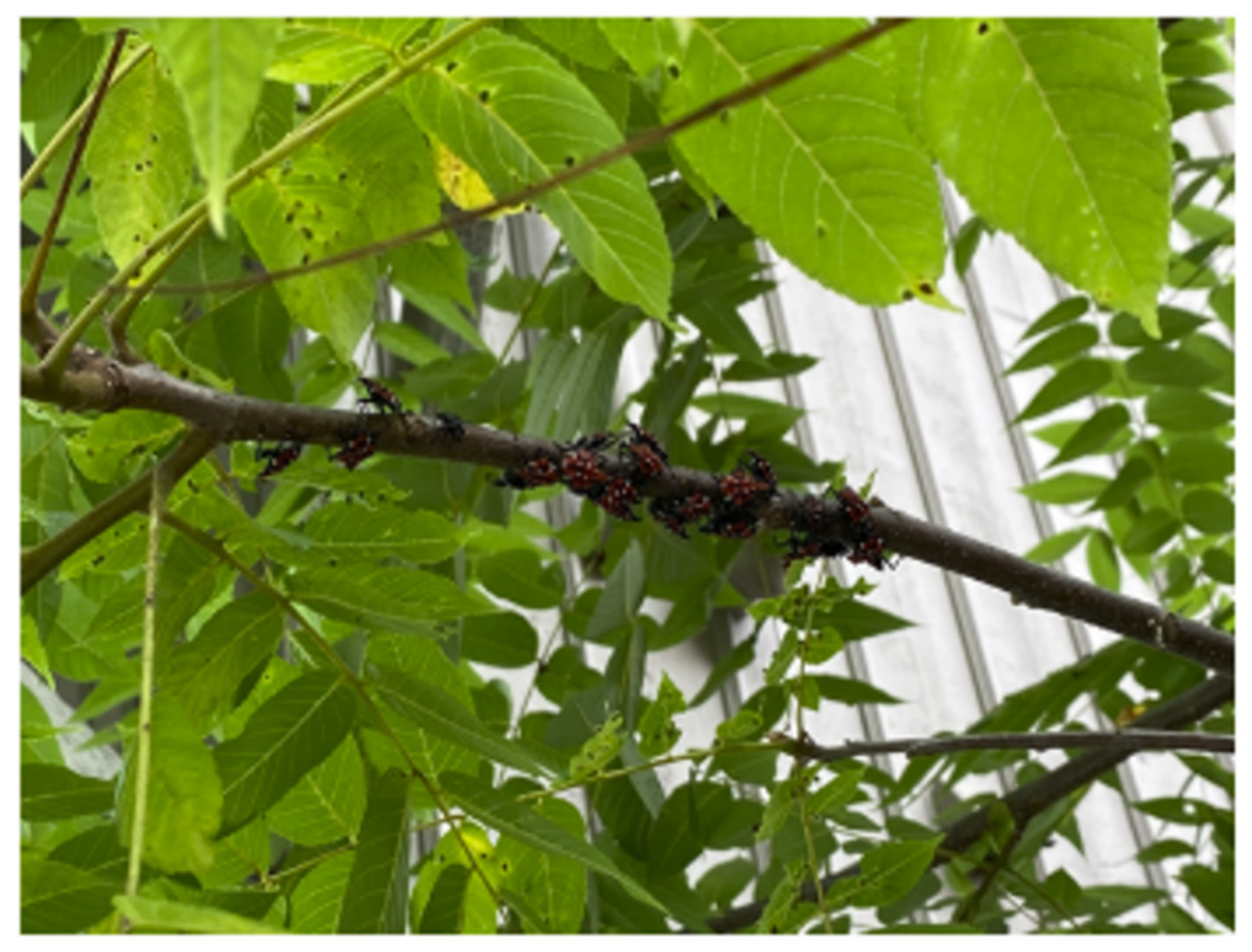
SLF nymphs clustered on a Black Walnut tree in the Clinton, NJ test site.
Figure 10.
SLF nymphs clustered on a Black Walnut tree in the Clinton, NJ test site.
Figure 11.
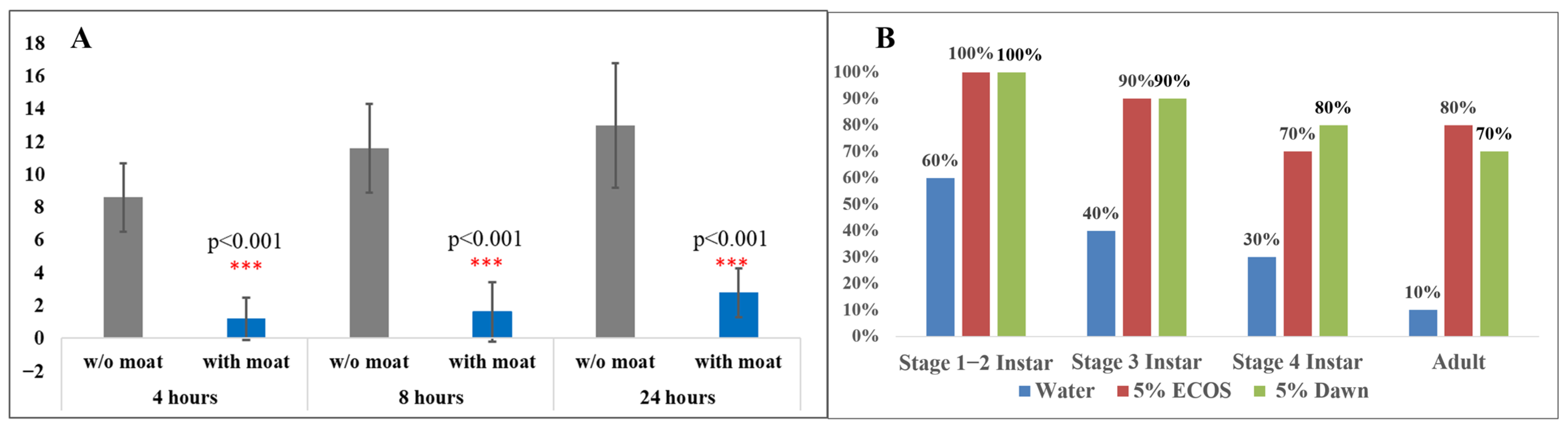
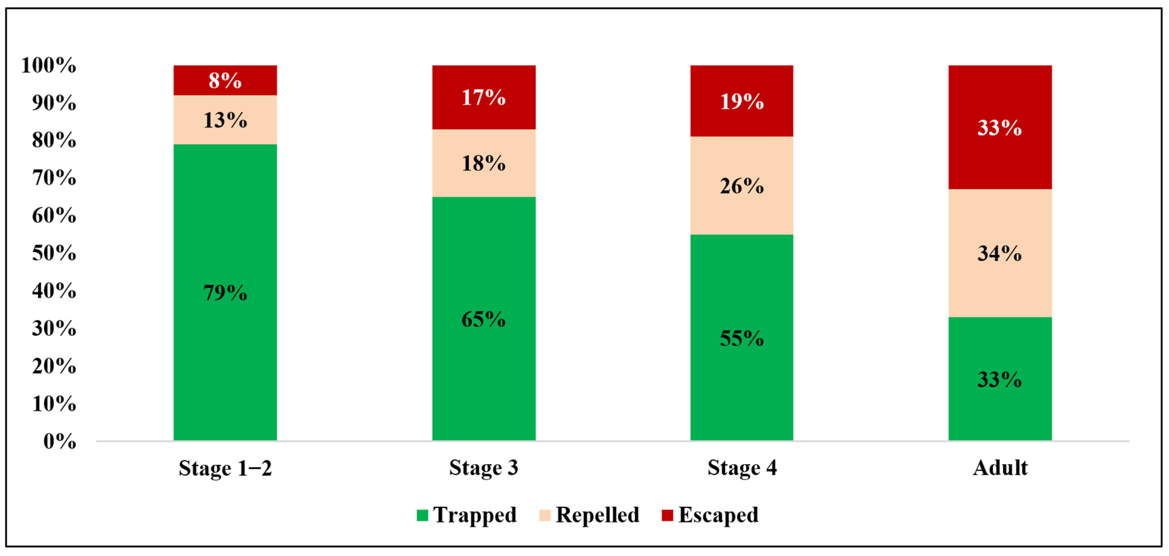
(A) Experimental results: the water moat significantly reduces the chance that SLF reach TOH branch. *** indicates p < 0.001. (B) Percentage of SLF that drown within one minute, by life stage.
Figure 11.
(A) Experimental results: the water moat significantly reduces the chance that SLF reach TOH branch. *** indicates p < 0.001. (B) Percentage of SLF that drown within one minute, by life stage.
Figure 12.
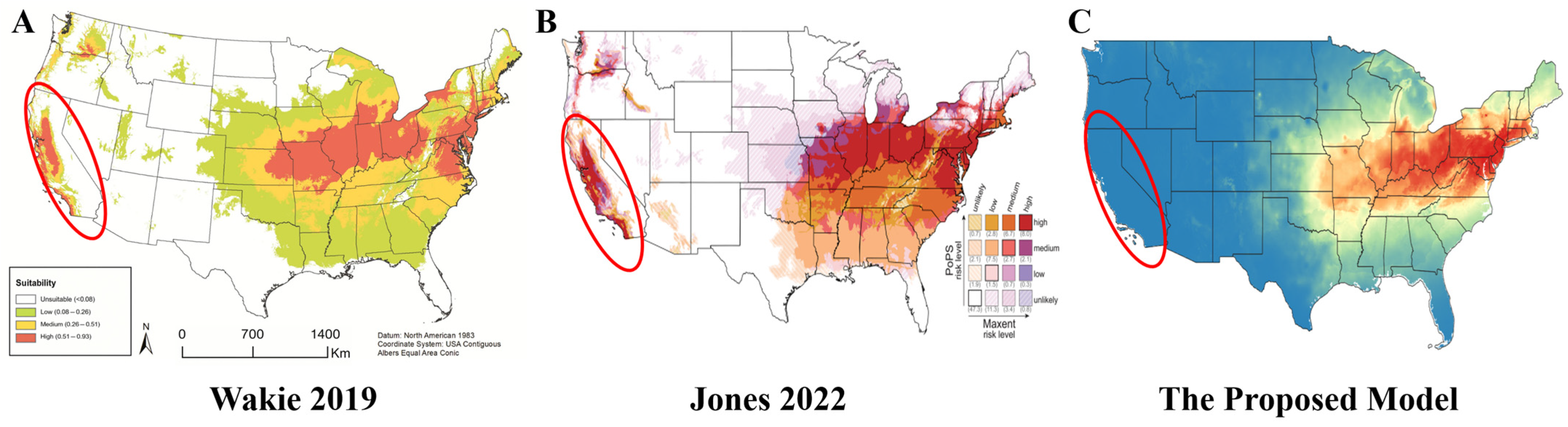
Unlike previous models from (
A) [
36] and (
B) [
7], (
C) AI-LyD suggests that the West Coast, particularly California (circled), is unlikely to face SLF invasion, consistent with current SLF proliferation trends. Panels (
A,
B) are reproduced from [
36] and [
7], respectively, under the Creative Commons Attribution (CC BY) license.
Figure 12.
Unlike previous models from (
A) [
36] and (
B) [
7], (
C) AI-LyD suggests that the West Coast, particularly California (circled), is unlikely to face SLF invasion, consistent with current SLF proliferation trends. Panels (
A,
B) are reproduced from [
36] and [
7], respectively, under the Creative Commons Attribution (CC BY) license.
Figure 13.
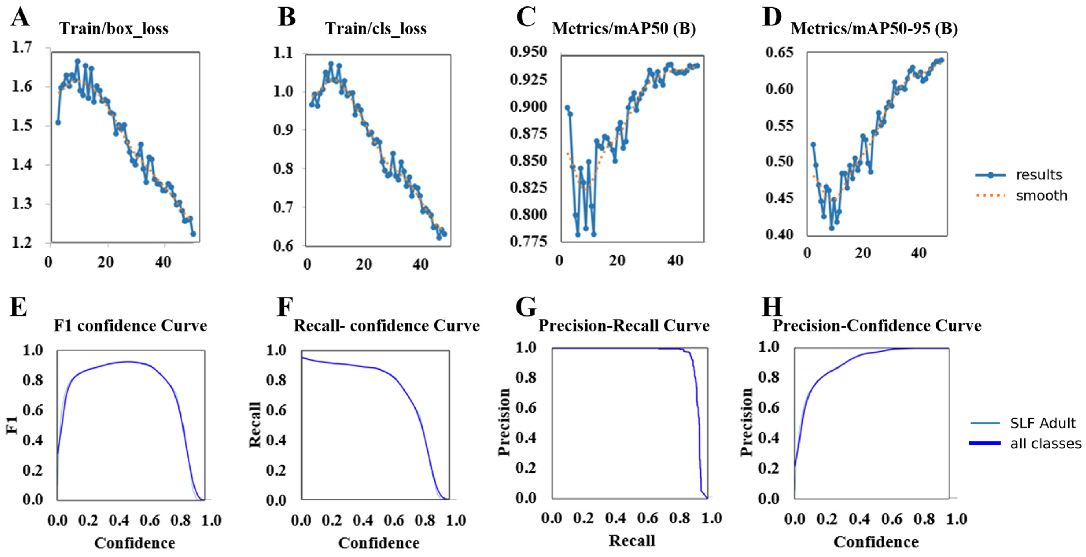
YOLO11 model’s training and performance metrics. (A,B) Training loss curves show improving box and class losses (C,D) Improvements reflected in mAP50 and mAP50-95 accuracy metrics (E–H) Performance evaluation curves across different SLF life stages.
Figure 13.
YOLO11 model’s training and performance metrics. (A,B) Training loss curves show improving box and class losses (C,D) Improvements reflected in mAP50 and mAP50-95 accuracy metrics (E–H) Performance evaluation curves across different SLF life stages.
Figure 14.
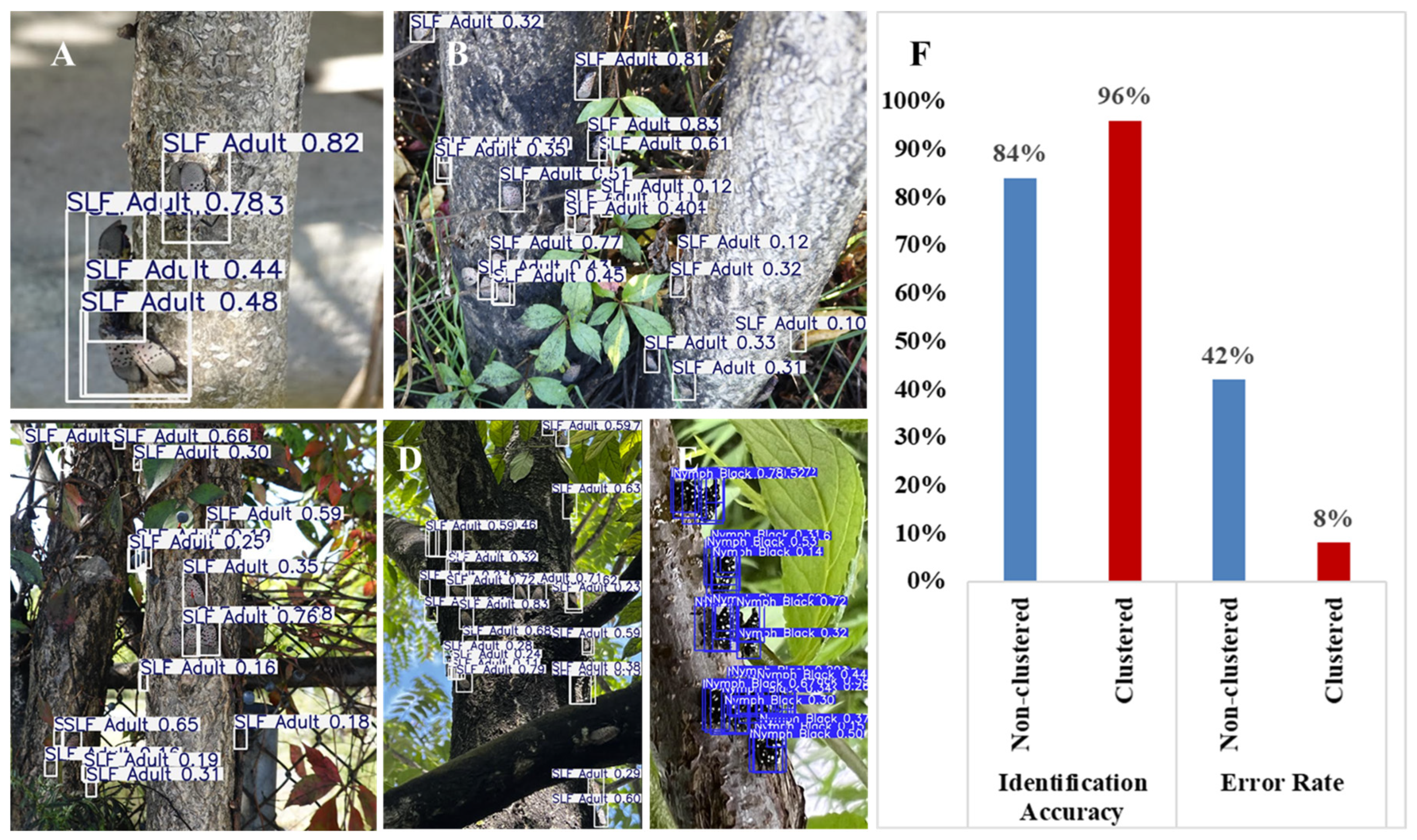
(A–F) SLF detection results from the clustered dataset demonstrate high confidence in its predictions. (B) Accuracy rate and error rate of detection models. Clustered SLF are more likely to be identified and with lower error rates.
Figure 14.
(A–F) SLF detection results from the clustered dataset demonstrate high confidence in its predictions. (B) Accuracy rate and error rate of detection models. Clustered SLF are more likely to be identified and with lower error rates.
Figure 15.
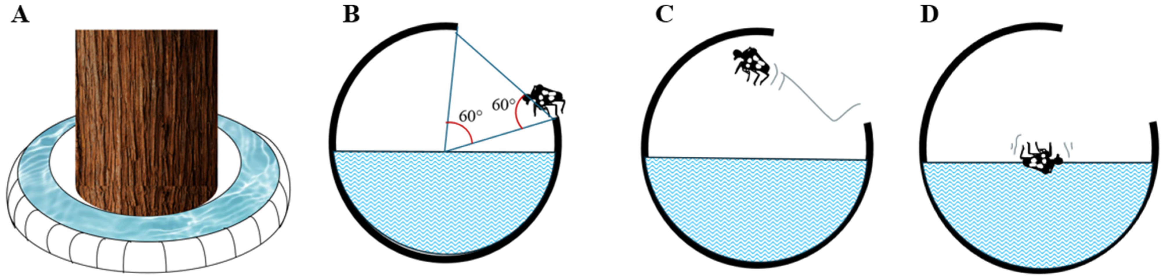
Aquabex’s design. (A) 3-D view of Aquabex. (B–D): Cross-sectional sequence of SLF jumping into Aquabex.
Figure 15.
Aquabex’s design. (A) 3-D view of Aquabex. (B–D): Cross-sectional sequence of SLF jumping into Aquabex.
Figure 16.
Aquabex’s efficiency in field comparison test.
Figure 16.
Aquabex’s efficiency in field comparison test.
Figure 17.
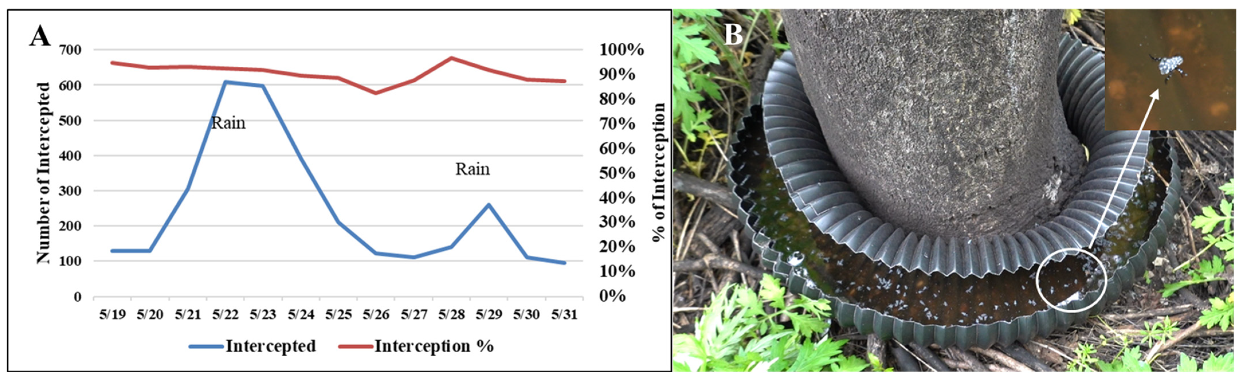
(A) Field test results from 19 May 2025 to 31 May 2025 of 12 Aquabex placed across 4 sites in Clinton, NJ (B) Aquabex capturing SLF.
Figure 17.
(A) Field test results from 19 May 2025 to 31 May 2025 of 12 Aquabex placed across 4 sites in Clinton, NJ (B) Aquabex capturing SLF.
Figure 18.
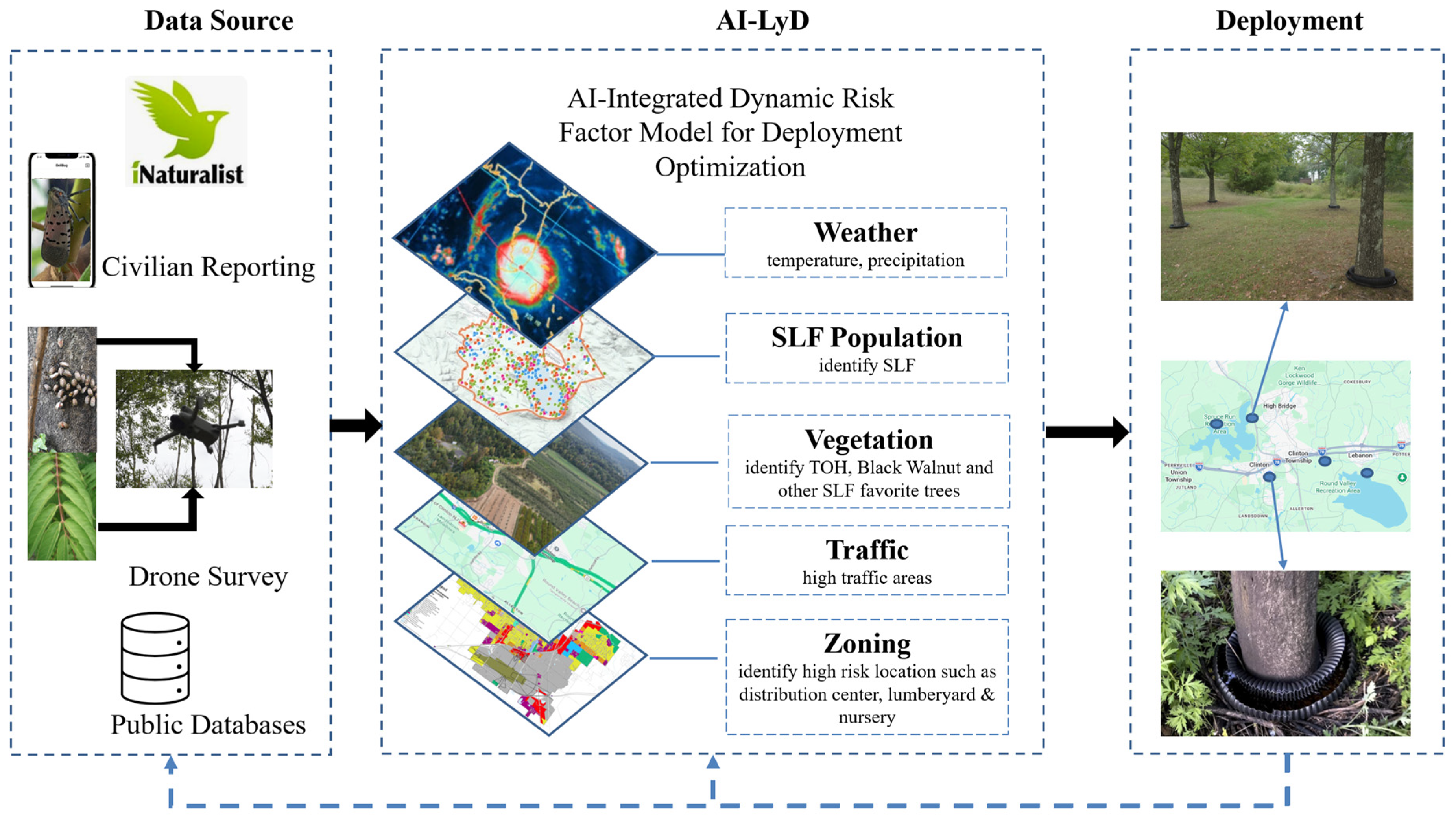
AI-LyD’s AI-driven Aquabex deployment plan, integrating multilayered spatial data for optimized mitigation.
Figure 18.
AI-LyD’s AI-driven Aquabex deployment plan, integrating multilayered spatial data for optimized mitigation.
Table 1.
Result of SLF egg hatching experiment.
Table 1.
Result of SLF egg hatching experiment.
| Hatching Start Date | No. Eggs Collected | No. Eggs Hatched | Hatch Rate | Average Hatching Duration (Days) |
|---|
| 6 November 2024 | 153 | 17 | 11% | 25 |
| 6 December 2024 | 135 | 43 | 32% | 31 |
| 6 January 2025 | 141 | 65 | 46% | 35 |
Table 2.
Representative sample of the SLF clustering experiment.
Table 2.
Representative sample of the SLF clustering experiment.
| Experiment No. | Number of Observed SLF (O) | Number of Expected SLF (E) | (O-E)2/E |
|---|
| Branch 1 | 18 | 4.29 | 43.89 |
| Branch 2 | 5 | 4.29 | 0.12 |
| Branch 3 | 2 | 4.29 | 1.22 |
| Branch 4 | 0 | 4.29 | 4.29 |
| Branch 5 | 1 | 4.29 | 2.52 |
| Branch 6 | 1 | 4.29 | 2.52 |
| Branch 7 | 0 | 4.29 | 4.29 |
| Total | 27 | 30 | |
| | | 53.83 |
| Degrees of Freedom (df) | | | 6 |
| p-Value | | | <0.0001 |
Table 3.
Summary of Chi-square significance test analyzing SLF clustering behavior across different host tree species.
Table 3.
Summary of Chi-square significance test analyzing SLF clustering behavior across different host tree species.
| Experiment No. | Tree Species | No. Observed SLF | No. Expected SLF | | df | p-Value | Significance |
|---|
| 1 | Styrax japonicus | 27 | 30 | 58.83 | 6 | <0.01 | *** |
| 2 | 26 | 30 | 20.00 | 6 | <0.01 | ** |
| 3 | Juglans nigra | 25 | 30 | 87.10 | 16 | <0.001 | *** |
| 4 | 28 | 30 | 150.80 | 16 | <0.001 | *** |
| 5 | Acer rubrum | 27 | 30 | 28.33 | 9 | <0.001 | *** |
| 6 | 25 | 30 | 22.33 | 9 | <0.01 | ** |
Table 4.
Summary of SLF return rates across experiments. The tree trunk serves as the primary pathway for SLF to return to their habitat.
Table 4.
Summary of SLF return rates across experiments. The tree trunk serves as the primary pathway for SLF to return to their habitat.
| | Experiment 1 | Experiment 2 | Experiment 3 | Experiment 4 | Experiment 5 | Experiment 6 | Total |
|---|
| Released | 30 | 30 | 30 | 30 | 30 | 30 | 180 |
| Returned | 27 | 26 | 25 | 28 | 27 | 25 | 158 |
| Return Rate | 90% | 87% | 83% | 93% | 90% | 83% | 88% |
Table 5.
Percentage of SLF that overcame the artificial barrier at varying angles, by life stage.
Table 5.
Percentage of SLF that overcame the artificial barrier at varying angles, by life stage.
| |
Stage 1–2 Instar
|
Stage 3 Instar
|
Stage 4 Instar
|
Adult
|
|---|
| <30° | 77% | 70% | 53% | 40% |
| <45° | 97% | 83% | 73% | 57% |
| <60° | 100% | 93% | 87% | 70% |
Table 6.
Percent contribution of various environmental layers.
Table 6.
Percent contribution of various environmental layers.
| Factor | Percent Contribution | Permutation Importance |
|---|
| Presence of Freezing Period | 59.3% | 17.6% |
| Precipitation During Warmest Quarter | 26.5% | 18.9% |
| Temperature Seasonality | 5.4% | 46.0% |
| Presence of TOH | 2.7% | 7.5% |
| Total annual precipitation | 0.7% | 9.9% |